124 FORECASTING IN FINANCIAL DATA CONTEXT
Mahmoud Dehghan Nayeri1† --- Ali Faal Ghayoumi2 --- Malihe Rostami3
1
Assistant Professor, Management and Economics Faculty, Tarbiat Modares University, Iran
2
Accounting Department, Shiraz University, Iran
3
Management Department, University of Grenoble, France
ABSTRACT
This paper aims to compare the application of most common forecasting techniques within financial data context such as regression analysis and artificial neural network, according to the most popular forecasting efficiency
indices. Findings depicted that robust regression has an advantages over the least square regression and ANN, in financial data analysis because of outliers derived from business cycles. To this aim, relationship between earning
per share, book value of equity per share and share price as price model and earnings per share, annual change of earning per share and return of stock as return model scrutinized implementing robust and least square regressions
as well as ANN. Based on results, it can be concluded that the robust regression can provide better and more reliable analysis owing to eliminating or reducing the contribution of outliers and influential data. Therefore, robust regression outperforms OLS and ANN, and can be recommended reaching more precise analysis in financial data
context.
© 2016 AESS Publications. All Rights Reserved.
Keywords: Forecasting, Financial data, Outlier, Robust regression, Efficiency, ANN.
Received: 28 January 2016/ Revised: 12 April 2016/ Accepted: 16 April 2016/ Published: 20 April 2016
Contribution/ Originality
This study contributes in the existing literature of financial forecasting models. Since it compare two common forecasting techniques with robust regression analysis based on the most important forecasting indices and clarified that robust analysis outperforms the other techniques because of the existence of outliers in financial data context.
1. INTRODUCTION
A statistical method commonly used in forecasting financial data is the regression analysis which often employs the least square regression (OLS) as its main means. However, as is obvious much deviation is experienced in financial data because of changes in financial policies and commercial cycles that inevitably gives rise to outlier observations in overall data (Ohlson, 1995). Since the least square regression is vulnerable to such outlier observations that will ultimately affect results from this technique (Anderson and Sweeney, 1998; Chen, 2002) and this will end in wrong conclusion and misleading users. The vulnerability of OLS regression to outliers may result from the failure to meet substantial assumptions required for this model.
Asian Journal of Economic Modelling
ISSN(e): 2312-3656/ISSN(p): 2313-2884
The assumption of normality is a crucial basis for most statistical methods of data analysis. However, various papers have shown this is true only with 10%-15% of data. This may be attributed to non-normal distribution of errors or the effect of outliers in observations (Liang and Kvalheim, 1996). Outliers are the observations not fitted to the pattern developed by the majority of the data (Bamett and Lewis, 1993; Preminger and Franck, 2007). There are two attitudes in statistical modeling in dealing with outliers. The first takes into account the outliers and the second eliminates outliers. Many scholars believe using robust estimation is necessary where outliers are not eliminated from the statistical analysis (Liang and Kvalheim, 1996).
Another essential assumption in regression analysis is the constancy of the error variance which is called homoscedasticity. Outliers, even when the sample is large enough, can lead to the accumulation of error variance and give rise to heteroskedasticity which means the error variance is not constant (Rousseeuw, 1984).
In most cases, especially when data are acquired in a continuous period of time like time series analysis, as is true with financial data, the correlation of data will be probable (Field and Zhou, 2003). The correlation will make errors interdependent in the regression model and reject the assumption of independent errors. The rejection of the assumption will lead to the inflation of the R square (R2) and erroneous significance of the developed regressio n model (Rousseeuw, 1984). This situation indispensably necessitates using robust regression models (Field and Zhou, 2003). Hence, in order to cope with financial data as a time series analysis, it is necessary to use a regression model that is not vulnerable to outliers and prevent bias of outcomes. The robust regression is a good substit ution for the least square regression concerning this issue. According to above, this study aims to introduce the strength of robust regression in financial time series analysis, in order to encourage scholars and practitioners to deploy this technique as a mean of improving the quality of their analysis. Although there are a lot of state of the art techniques for forecasting such as Artificial Neural Networks (ANNs) with high rate of accuracy but the ration of statistical techniques and their analyzability make them in practice up to know.
In addition to above, ANN as a nonparametric technique which can learn the data nature like human brains do is used as a forecasting technique in comparing the efficiency of forecasting techniques within two popular financial models in Iran’s stock exchange. NNs cannot act as suitable as regression analysis for financial analysis and forecasting, because that the equations and the predicting coefficients are not clear in NNs which leads to weaker analyzability. Also there are not some validating statistical test for ensuring the estimated parameters where there are not estimated within NNs which makes it more unacceptable to practitioners. In the following, the paper after a short reviewing of the outliers, their roles in financial data analysis and robust regression as well as NNs, will compare these popular forecasting techniques in case of two financial models (Return and Price model) and their strengths and weakness will be concentrated.
2. LITERATURE REVIEW
In this section, firstly outliers, their types and dominions will be discussed. Subsequent to grasping the concept of outliers, number of robust regression techniques that can attenuate the role of outliers will be introduced. To formulate a robust regression model one should not restrict out an observation to some isolated sporadic cases but should identify outliers and influential data in order to reduce or eliminate their effects (Chatterjee and Hadi, 2006). In the following, the paper has provided NNs in summary within section D and the most common forecasting efficiency indices through section E.
2.1. Outliers
Outliers are the observations concomitant of high error residual (Gujarati, 1995). The error volume is equal to the difference between the observed quantity and the predicted quantity for ith observation. This can be derived from:
The summation of errors is zero in a regression technique but the variance of errors can be different. This difference reduces the significance of comparing models. To overcome inequality of the error variance, their standardized values are used (Anderson and Sweeney, 1998; Martin, 2002). Standardized errors usually have a normal distribution with zero mean value and standard deviation of 1. The points with standardized error more than 2 or 3 and the standard deviation beyond the mean value (zero) are regarded as outliers (Martin, 2002).
Drawing diagrams is another technique to identify outliers. In this method, a distribution diagram or estimated deviation diagram is prepared, and the points away from the concentration of points or the regression line are outliers (Azar and Momeni, 2008). Figure 1 depicts a number of data, as well as an outlier. It should be noted where we have a great deal of data we will face more constraints in using the schematic presentation.
Fig-1. Identifying an outlier by means of a diagram
Source: Author
Based on this introduction, if the deviation of an error is too large it is designated as an outlier. Therefore, the value of the dependent variable is a quantity used to identify outliers. Another type of outliers that are called influential data are investigated in relation to independent variables, that is, if a data much different from the average of data as concerned the independent variable it is an influential data (Martin, 2002).
2.2. Influential Observations
Sometimes, one or more data have remarkable effect on estimated parameters of a regression model. These are known as influential data (Chatterjee and Hadi, 1986). In other words, influential data are the data whose removal from the model will give rise to crucial alteration in the model though eliminating every observation introduces a change in the regression model, but when there are notable changes (including change in the slope or intercept) that observation will be influential (Martin, 2002). Figure 2 shows an influential data beside the regression line. The regression line in this diagram has a negative slope, and if the influential observation is removed the line’s slope will become positive and the intercept will reduce. Evidently, this observation has a greater role in determining the estimated regression.
The leverage value can be employed to find out influential observations. The leverage value is the difference in the magnitude of independent variables from their mean value. The leverage value for ith observation is calculated using this formula:
̅
∑ ̅
Where n is the number of observations, is ith observation, ̅ mean value of observations and the leverage value of ith observation.
Usually, the points with the leverage value two times the average of leverage values are known as the points with high leverage value (influential) (Hoaglin and Welsch, 1978). Of course, some researchers admit the points with a leverage value above 0.5 as the influential data (Chatterjee and Hadi, 2006). Statistical tests have been developed for the identification of influential observations. Almost all of these tests use the leverage value as a main tool. One of the most famous tests is the Cook’s distance measure (Cook, 1977). The Cook’s distance measure uses both the leverage value and the error magnitude to measure the extent of influence of the data. The equation 3 shows how this test is calculated:
∑ [ ] (3)
In this equation, K denotes for the number of independent variables, and Se denotes the standard error of estimation. To know further about this technique, the reader is advised to see the Chatterjee and Hadi (1986).
2.3. Robust Regression
Robust regression is the regression that tries to minimize or eliminate the effect of outliers or influential data in order to provide a more reliable estimation based on the majority of data. In other words, robust regression is an attempt to find real results out of most data (Martin, 2002). Hence, various types of robust regression fall in the category of robust estimation methods that function through eliminating or moderating the effect of outliers (Liang and Kvalheim, 1996). It was noted earlier that the normality of errors is one of the primary assumptions in regression
models but there is always some divergence from this assumption. In such cases, robust regression can be a substitute for the least square method which is less susceptible to the divergence (Rousseeuw, 1984). The OLS regression is not immune to outliers owing to its objective-oriented nature of the OLS. This fact is illustrated in the equation 4 that shows the minimum of the summation of errors.
∑ ∑
Where stand for error, for the dependent variable and the independent variable and {θ j , j=1,…,m} are the parameters estimated by the OLS model (Liang and Kvalheim, 1996).
The model’s susceptibility to the error square is obvious; hence outliers significantly contribute to the formation of parameters.
Edgeworth (1887) pioneered the development of the robust regression. He pointed out that outliers, owing to becoming square, crucially impress the OLS. Therefore, he presented the least absolute deviation model (equation 5) ((Ohlson, 1995).
∑| |
Hodges (1967) introduced the concept of breakdown point in order to help assessing the robust regression’s stability toward outliers. Rousseeuw and Leroy (1987) defined breakdown point as the lowest ratio of outliers that can impair the regression model. The higher the breakdown point in a regression model, the more satisfactorily model functions. For L1 and L2, the breakdown point is equal to 1/n. In other words, as the result of the existence of an outlier in a set of data, it can render invalid the model by errors (Liang and Kvalheim, 1996).
There are various types of robust regression that with different functions try to provide a stable model. Choosing which robust regression is suitable for a case depends on the nature of data and the discretion of the persons using the regression (Liang and Kvalheim, 1996).
Next to LAD, least trimmed square (LTS) is another type of robust regression. This regression, introduced by Rousseeuw for the first time in 1984, is a technique to eliminate possible outliers (Rousseeuw and Van Driessen, 1998). Coefficients in the equation of the least trimmed square regression are estimated similar to the ordinary regression (least square). In other words, the coefficients in these two types of regression are estimated in a way to minimize the summation of the second power of errors. However, in least trimmed square, unlike the ordinary regression, not all data is used in estimating the regression model but the data accompanied with high errors are eliminated (Rousseeuw, 1984).
The equation 6 explains how data are selected and which mechanism is used in least trimmed square to estimate the equation (Rousseeuw and Leroy, 1987).
∑ ̂
⁄
Where is the number of observations, the value of ith observation, ̂ the anticipated value of ith observation, q is the number of the data used in least trimmed regression equation, and k the number of parameters including the intercept.
To find the data required to estimate the least trimmed square regression, the second power of each observation is calculated. Then, these values are arranged in an ascending order. Finally, the observations with least error square are selected and this procedure continues up to the observation q.
It should be noted that in some statistical software programs (like S-PLUS), if the data used in estimating the least trimmed square regression is less than 90% of the data, only the 90% of the data are used in estimating the equation. Some researches doubt the reliability of such regressions (Li et al., 2010) though this regression has improved owing to the introduction of another initiative called the rapid least trimmed square that was set forth by Rousseeuw and Van Driessen (1998); Rousseeuw and Leroy (1987).
Another version of robust regression is the iteratively reweighted least square that was presented by Chatterjee and Mächler (1997). In iteratively reweighted least square regression, the points with high leverage value and high error are almost prevented from contributing to the outcome in a lesser extent in order to reduce their effects on results of the regression analysis. In this regression, the weight of ith observation is calculated from this equation:
(| | | |)
Where denotes the weight of ith observation, the leverage value of the ith observation, the error with
the ith observation, and | | the average of the absolute value of errors.
2.4. Artificial Neural Network
ANN usually called ―neural network‖ (NN), is a mathematical model or computational model that tries to simulate the structure and/or functional aspects of biological neural networks. It consists of an interconnected group of artificial neurons and processes information using a connectionist approach to computation. In most cases an ANN is an adaptive system that changes its structure based on external or internal information that flows through the network during the learning phase. Modern neural networks are non-linear statistical data modeling tools. They are usually used to model complex relationships between inputs and outputs or to find patterns in data (Li et al., 2010).
Although lots of architecture for designing neural network models can be developed, in this study a feed forward neural network is deployed for data analyzing which is mentioned as the most popular and most widely used model in many practical applications (Li et al., 2010). The model is developed based on three layers, one input, one output and a hidden layer. The number of neurons developed based on the data nature in input and output layer, and neuron number of hidden layer set as (2×n + 1) based on Kolmogorov Theorem. In which, denotes to the number of input layer neurons.
2.5. Forecasting Efficiency Indices
After introducing Robust regression and NNs, this section aims to review the forecasting accuracy indices, which are widely have been used, including the root mean square error (RMSE), mean absolute error (MAD), mean absolute percentage error (MAPE), and the success rate (SR) that counts the number of right forecast of the sign of the true value by the model (Ohlson, 1995). If and ̂ are taken as the true value and the anticipated value in period and proportionally calculate the forecast from i+l to i+n period then the equations for calculating abovementioned indices will be as follows:
√ ∑ ̂
∑ | ̂ |
∑ ̂
∑ | ̂|
3. RESEARCH METHODOLOGY
This is an experimental and developmental research, in category of casual correlation researches with the goal of forecasting improvement. It also tries to show the strength and capability of robust regression in analyzing financial data. Ultimately, it tries to prevent probable bias that may be produced by the least square regression in time series forecasting. In this case, the input of the study is the data collected from 135 companies in the Tehran stock exchange in the period 2002-2009. These data have been gathered cumulatively and include 1080 company-year data.
and its annual change. To this aim, OLS, IRILS and LTS regression models and NNs are used for developing above mentioned models. Ultimately comparisons within all models are provided. Statistical analyses have been carried out using SPSS and S-PLUS statistical tools.
3.1. Deployed Models
In this research, developing regression models and collecting data have been based on two Return model and Price model. The Return model illustrates the relation between the stock return and accounting profit, and includes dividend per stock and fluctuations in the dividend as independent variables. This model which was presented by Easton and Harris can be described as follows (Easton and Harris, 1991):
(12)
In this model, is the annual yield of the company, denotes dividend, changes in dividend per
stock and is the last year’s stock prices.
Another model, which is known as the Price model, was introduced by Ohlson for the first time in 1995 (Neter et al., 1996). This model explains the relation between the stock price and two independent variables – dividend per stock and the book value of stocks – and can be shown in the equation 13.
(13)
In this model, is the market value of stocks from the company at the end of the month of presenting financial statements, stands for the book value of each stock of the company , and is the accounting profit
reported for each stock of the company in period .
All variables of the presented study, excluding the book value, have been calculated for each company. The stock return variable has been calculated from the difference between the price of a stock at the end of the month of presenting financial statements of the company in the last year and the price of a stock at the end of the month of presenting financial statements in the current year plus yields (including the dividend, reward) proportional to the price of a stock price at the end of the month of presenting financial statements in the last year. In the next section, we will discuss the result of employing these various types of regressions and NNs in estimating related models and will compare their performance in order to ultimately choose the most favorable forecasting technique.
4. FINDINGS AND CONCLUSION
Results of regression analysis according to the Price model are presented in table 1. As it is clear, the adjusted determination coefficient in the least square regression is equal to 0.474 that shows independent variables of the model (dividend arising from each stock and the book value of the stocks) explains for 47% of the changes in the dependent variable (stock price). Furthermore, the t-student test shows the insignificance of the book value variable at the level of 5%. In other words, there is no significant relation between the stock price and the stock book value.
Table-1. Results of the Regression Analysis for the Price Model T- Test β EPS BV EPS BV R2 Model P-value T P-value T 0.00 28.54 0.37* 0.89 5.56 0.19 0.47 OLS ---3.56 0.42 0.62 LTS 0.00 46.59 0.02 2.31 5.09 0.23 0.72 IRLS
* BV is rejected in OLS regression analysis
The difference between results of these three regressions can be explained in the light of reducing the effect of outliers and influential data. These data damages the efficiency of the model and the lever of significance of one of independent variables in the lease square regression. Based on this, if the researchers relies on the least square regression to draw result he will go wrong and the analysis will end in false findings. Consequently, it can be concluded that robust techniques will provide more satisfactory results and we will discuss this later. It is clear that by using IRLS the r-square is increased to 0.72 from 0.47 of OLS which means that the IRLS is more powerful in determining the dependent variable.
Table 2 shows the result of regression analysis for the Return model. The adjusted coefficient in the least square regression is about 0.14. In other words, only 14% of changes in the dependent variable (stock return) can be explained by independent variables (dividend for a stock and the book value of stocks).
In LTS regression technique, independent variables are able to explain the stock return somewhat better. Of course, in the IRLS this improvement is remarkable and is about 24%. A comparison of regression analyses in the Return model shows that reducing the impact of outliers and influential data improves the efficiency of the model. It must also be noted that using robust regression does not always lead to enhancement of results of a regression analysis but it helps making the results more realistic. Anyway, all the employed techniques are significant with respect to the F test.
Table-2. Results of the Regression Analysis for the Return Model
T- Test β
R2
Regression EPS/P ΔEPS/P
EPS/P Δ EPS/P P-value T P-value T 0.0 5.23 0.00 8.06 32.06 110.99 0.139 OLS ---19.08 115.25 0.142 LTS 0.0 6.86 0.00 11.28 32.24 111.65 0.244 IRLS
Source: Author’s calculation
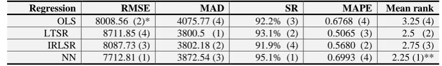
We have used the same criteria of assessment described in the section E of Literature, in order to scrutinize the performance of the developed models according to employed techniques. Calculation of the related indices for abovementioned regression techniques in addition with NN method for both Price and Return model is depicted in tables 3 and 4 respectively. In evaluating the techniques, the lower RMSE, MAD and MAPE indices, and the more the SR index, will lead to the more desirable considered technique.
Table-3. Comparison of OLS, IRLS and LTS Regression and NN in Price Model
Mean rank MAPE SR MAD RMSE Regression 3.25 (4) 0.6768 (4)
92.2% (3) 4075.77 (4)
8008.56 (2)* OLS
2.5 (2) 0.5065 (3)
93.1% (2) 3800.5 (1)
8711.85 (4) LTSR
2.75 (3) 0.5680 (2)
91.9% (4) 3802.18 (2)
8087.73 (3) IRLSR
2.25 (1)** 0.6993 (4)
95.1% (1) 3872.54 (3)
7712.81 (1) NN
As is seen, as MAD, MAPE and SR indices are concerned robust technique have functioned better than OLS. The value of SR for OLS regression is approximately 92%. The most favorable value is 100% and shows all predictions are of the same sign with real values. From the value 92% it is inferred that in 8% of cases the sign of the predicted value is contrary to the sign real values. In other words, the model is extremely weak in 8% of cases.
On the other hand, the result is inversed when RMSE index is used as a criterion for comparison. It can be concluded that robust model’s performance is less satisfactory when this index is measured. However, in order to prevent the accumulation of outlier-simulated error in RMSE it is recommended to use the MAD index. Some researchers approve using this initiative (Liang and Kvalheim, 1996).
The ranking of techniques according to different Indices depicted that although there are some deviations, but as a whole NN is more efficient than robust techniques and the worst efficient technique is OLS regression according to Mean ranking.
Table-4. Comparison of OLS, IRLS and LTS Regressions and NN in Return Model
Mean rank MAPE
SR MAD
RMSE Regression
3.00 (2) 7.620 (4)
65.2% (3) 52.92 (4)
82.49 (1)* OLS
2.66 (1)** 4.741 (1)
65.3% (2) 50.03 (1)
84.98 (4) LTSR
2.66 (1)** 5.848 (2)
65.4% (1) 50.51 (2)
83.30 (3) IRLSR
3.00 (2) 7.313 (3)
64.6% (4) 51.74 (3)
82.92 (2) NN
* Rank **Most efficient Robust technique
In Return model the results are different. In this model the robust techniques are more efficient than both NN and OLS. It can be concluded that according to the data itself the efficiency of forecasting techniques may differ, but in both cases the robust technique outperform the OLS in financial data, which may be because of the outliers that explained before in the nature of financial data. As the findings provided except RMSE the robust techniques are more favorable than the others.
It is clear that according to the findings, the fact that robust techniques are more suitable than OLS for financial data. The nature of financial data are full of business cycles, regulatory constraints, temporary growth times, changes in financial policies and commercial cycles which inevitably gives rise to outlier observations in overall data. To cope with these problems, practitioners should use robust regression techniques instead of ordinary least square techniques to avoid misleading results.
In comparing Robust regression models with NN, it can be concluded that although NN can forecast the financial data and time series with a high rate of accuracy but some inherent shortcomings of NN, makes it difficult to be deployed as an analytical tool for financial engineering purpose. Apart from defining the general architecture of a network and perhaps initially seeding it with a random numbers, the user has no other role than to feed it input and watch it train and the output. Somehow the user even doesn’t know about the algorithm and this can lead to misuse of the NN. In addition to that the final product of this activity is a trained network that provides no equations or coefficients defining a relationship (as in regression) beyond its own internal mathematics. The network 'IS' the final equation of the relationship. It means that by the NN product the user cannot manipulate and design alternative strategies to check the outcome which can be done easily with regression equations. Ultimately by reviewing some popular forecasting models in practical financial forecasting, it is clear that Robust regression by combining the power of efficient forecasting and producing analytical equation can outperform the other regression and NNs models within financial data analyzing.
Funding: This study received no specific financial support.
Competing Interests: The authors declare that they have no competing interests.
REFERENCES
Anderson, D.R. and D.J. Sweeney, 1998. Statistics for business and economics. 7th Edn., South Western College: Williams, T.A.
Azar, A. and M. Momeni, 2008. Business statistics. 3rd Edn., Tehran: Samt Publications.
Bamett, V. and T. Lewis, 1993. Outliers in statistical data. 3rd Edn., Chichester: Wiley.
Chatterjee, S. and A.S. Hadi, 1986. Influential observations, high leverage points, and outliers in linear regression. Statical
Science, 1(3): 379-416.
Chatterjee, S. and A.S. Hadi, 2006. Regression analysis by example. 4th Edn., New Jersey: Wiley.
Chatterjee, S. and M. Mächler, 1997. Robust regression: A weighted least squares approach. Communications in Statistics —
Theory and Methods, 26(6): 1381–1394.
Chen, C., 2002. Robust regression and outlier detection with the ROBUSTREG procedure. Presented at SUGI, No. 27.
Cook, R.D., 1977. Detection of influential observations in linear regression. Technometrics, 19(1): 15-18.
Easton, P. and T. Harris, 1991. Earnings as an explanatory variable for returns. Journal of Accounting Research, 29(1): 19–36.
Edgeworth, F.Y., 1887. On observations relating to several quantities. Her-mathena, 6(13): 279-285.
Field, C. and J. Zhou, 2003. Confidence intervals based on robust regression. Journal of Statistical Planning and Inference, 115(2):
425 – 439.
Gujarati, D.N., 1995. Basic econometrics. 3rd Edn., New York: McGraw-Hill International Edition.
Hoaglin, D.C. and R.E. Welsch, 1978. The hat matrix in regressin and ANOVA. American Statistician, 32(1): 17-22.
Hodges, J.L., 1967. Proc. Fifth Berkeley Symp. Math. Stat. Probab. No. 1: 163-168. Available from
http://www.2sas.com/proceedings/sugi27/pdf.
Li, G., S. Xu and Z. Li, 2010. Short-term price forecasting for agro-products using artificial neural networks. Agriculture and
Agricultural Science Procedia, 1: 278-287.
Liang, Y.Z. and O.M. Kvalheim, 1996. Robust methods for multivariate analysis - a tutorial review. Chemometrics and Intelligent
Laboratory Systems, 32(1): 1-10.
Martin, R.D., 2002. Robust statistics with the S-Plus robust library and financial applications. New York, NY: Insightful Corp
Presentation, No.17-18, 1 and 2.
Neter, J., M.H. Kunter, C.J. Nachtsheim and W. Wasserman, 1996. Applied linear regression models. 3rd Edn., USA:
McGraw-Hill.
Ohlson, J., 1995. Earnings, book values, and dividends in equity valuation. Contemporary Accounting Research, 11(2): 661–687.
Preminger, A. and R. Franck, 2007. Forecasting exchange rates: A robust regression approach. International Journal of
Forecasting, 23(1): 71– 84.
Rousseeuw, P.J., 1984. Least median of squares regression. Journal of the American Statistical Association, 79(388): 871-880.
Rousseeuw, P.J. and A.M. Leroy, 1987. Robust regression and outlier detection. New York: Wiley.
Rousseeuw, P.J. and K. Van Driessen, 1998. Computing LTS regression for large data sets. Technical Report, University of
Antwerp.