DOI: 10.1534/genetics.108.088070
Within-Generation Mutation Variance for Litter Size in Inbred Mice
Joaquim Casellas* and Juan F. Medrano
†,1*Gene`tica i Millora Animal, Institut de Recerca i Tecnologia Agroalimenta`ries-Lleida, 25198 Lleida, Spain and†Department of Animal Science, University of California, Davis, California 95616-8521
Manuscript received February 14, 2008 Accepted for publication May 30, 2008
ABSTRACT The mutational input of genetic variance per generation (s2
m) is the lower limit of the genetic variability in inbred strains of mice, although greater values could be expected due to the accumulation of new mutations in successive generations. A mixed-model analysis using Bayesian methods was applied to estimates2
mand the across-generation accumulated genetic variability on litter size in 46 generations of a C57BL/6J inbred strain. This allowed for a separate inference ons2
mand on the additive genetic variance in the base population (s2
a). The additive genetic variance in the base generation was 0.151 and quickly decreased to almost null estimates in generation 10. On the other hand,s2
mwas moderate (0.035) and the within-generation mutational variance increased up to generation 14, then oscillating between 0.102 and 0.234 in remaining generations. This pattern suggested the existence of a continuous uploading of genetic variability for litter size (h2¼0:045). Relevant genetic drift was not detected in this population. In conclusion, our approach allowed for separate estimation of s2
a and s2m within the mixed-model framework, and the heritability obtained highlighted the significant and continuous influence of new genetic variability affecting the genetic stability of inbred strains.
T
HE importance of new mutations on polygenic variability has been suggested by several investi-gators in the last decades (Hill 1982a,b; Caballero et al. 1991; Keightley 1998). Direct evidence of newmutations with large effects in experimental selection lines was initially reported during the second half of the 20th century (Macarthur1949; Yoo1980; Bradford
and Famula 1984). The mutational input of genetic
variance per generation (s2
m) can be viewed as the ultimate source of polygenic variation and thus as the raw material for the maintenance of genetic variability in populations (Hill 1982a). Estimates of mutational
heritabilities [h2 m¼s
2 m=ðs
2 m1s
2 eÞ, s
2
e being the resid-ual variance of the trait] in animals and cereal crops have ranged between 104 and 53102(Lynch1988; Houleet al. 1996). Within this context, it is well known
that spontaneous mutation continually contributes new alleles to the pool of genetic variation, allowing for re-sponse to long-term artificial selection experiments in both animals (Caballeroet al. 1991; Keightley1998)
and plants (Hill2007).
Most estimates ofs2 mandh
2
mcome from experiments focused on the rate of divergence between sublines from a highly inbred base population (Festing1973; Mackay et al. 1994). These studies typically assumed a stringent scenario under mutation–drift equilibrium, which does not necessarily hold in experimental populations (Hill
1982a). Moreover, a long time is needed for generating the strains, and the analysis using the response to selection typically ignores information on covariances between relatives within lines, a proportion of which can be genetic (Keightley and Hill 1992). Alternatively,
Wray(1990) developed a straightforward approach to
account for mutation effects in mixed models, using the numerator relationship matrix, allowing for estimation ofs2
min unselected populations. This methodology has not been widely applied, although some s2
m estimates have been obtained in mice (Keightleyand Hill1992;
Keightley 1998). A topic of interest in studies with
laboratory mice is the genetic homogeneity of inbred strains across generations (Taftet al. 2006; Stevenset al.
2007) and Wray’s (1990) approach seems to be the only
available methodology for testing mutation effects, given that selection is avoided in these genetically controlled strains. Nevertheless, there are no published results ons2
min highly inbred unselected mice, and the magnitude or impact ofs2
mon the phenotypic variance remains unknown.
Taking the infinitesimal model (Fisher1918) as the
starting point, the additive genetic variance for a given phenotypic trait in a population characterizes the amount of genetic variability and the potential change due to natural or artificial selection, or genetic drift. Interest-ingly, analyses performed on the ‘‘new’’ genetic variance originated by mutation are commonly focused on the increment of genetic variation per generation (Caballero et al. 1991; Keightley1998), but they do not estimate
the accumulated genetic variability existing between 1Corresponding author:Department of Animal Science, University of
California, One Shields Ave., Davis, CA 95616-8521. E-mail: [email protected]
individuals. Even in highly inbred strains, the genetic variance in a given generation of interest could be viewed as the balance of an equilibrium between s2
m coming from current and previous generations and the loss of genetic variability due to selection, genetic drift, and/or inbreeding (Hill 1982a,b). Analyses of the
mutation phenomenon in laboratory species have been mainly focused ons2
m (Festing1973; Keightleyand Hill1992; Keightley1998), whereas the magnitude of
the overall within-generation genetic variability due to the accumulation of new mutations remains unclear.
In this study, we report estimates of mutation variance on litter size in C57BL/6J mice reared for 46 gener-ations without selection. Wray’s (1990) algorithm was
modified to estimate the amount of genetic variance in the inbred base population and the increment of the per generation variance due to mutation. In addition, we applied the Bayesian approach proposed by Sorensen et al. (2001) to estimate the within-generation genetic variability, to examine if new mutation variance com-pensates for losses in genetic variability.
MATERIALS AND METHODS
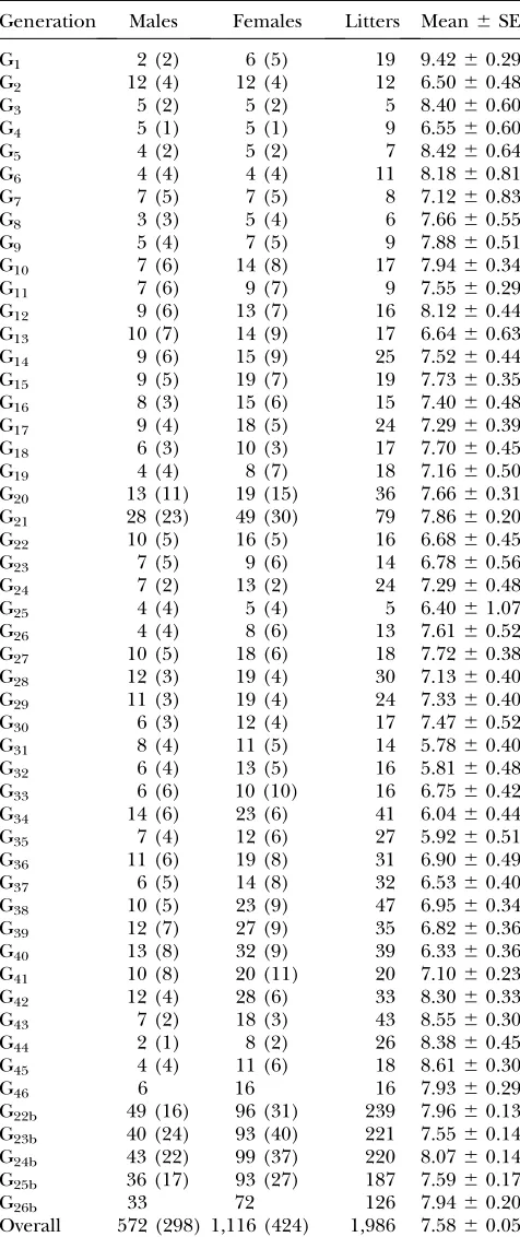
Mice data source: Mouse strain and breeding scheme: A C57BL/6J inbred strain was kept in our vivarium at the University of California (Davis, CA) for 46 nonoverlapping generations (G1–G46), between October 1988 and May 2005. This strain was founded with two C57BL/6J males and six C57BL/6J females from The Jackson Laboratory (Bar Harbor, ME). Two to 5 generations per year were produced. Each generation involved between 2 and 28 males and between 6 and 49 females, producing an average of 21.6 litters (Table 1). In August 1995, a subline was derived from G21 and was maintained for five nonoverlapping generations (G22b–G26b), with a large number of litters per generation (Table 1). For each generation, males and females were selected at random from the offspring of a few litters of the previous generation, and full-sibs matings were favored. Only single (one male/one female) and group matings (one male/several females) were used to avoid multiple paternities. Each male and female produced an average of 3.5 and 1.8 litters, respectively, ranging from 1 to 16 litters for males and from 1 to 5 litters for females. Note that this strain was maintained to provide stock research mice in our colony and therefore a variable number of litters per generation were generated, depending on mice demand. All mice were fed with Purina 5008 diet (Ralston Purina, St. Louis; 23.5% protein, 6.5% fat, 3.3 kcal/g) and water was offeredad libitum. Mice were housed in polycarbonate cages under controlled conditions of temperature (21° 6 2°), humidity (40–70%), and lighting (14 hr light, 10 hr dark, lights on at 7am) and managed according to the guidelines of the American Association for Accreditation of Laboratory Animal Care (AAALAC) (http://www.aaalac.org).
Data set and trait analyzed:Reproductive data were recorded accurately in all generations. Sire, dam, date of mating, date of birth, and number of pups at birth (alive and dead) were recorded for each litter, and pups were individually marked by ear notching at weaning (3 weeks after birth). Records were available on 1986 litters providing 15,044 pups. This study focused on litter size (LS), defined as the sum of live and dead pups at birth. Phenotypic records of LS ranged between 1 and
14 pups, with 7.58 pups per litter on average. The pedigree file included 572 males and 1116 females with a complete knowledge of all parental relationships.
TABLE 1
Number of males and females mated per generation (in parentheses, contributors to the next generation), number
of litters, and average litter size per generation
Generation Males Females Litters Mean6SE
G1 2 (2) 6 (5) 19 9.4260.29
G2 12 (4) 12 (4) 12 6.5060.48
G3 5 (2) 5 (2) 5 8.4060.60
G4 5 (1) 5 (1) 9 6.5560.60
G5 4 (2) 5 (2) 7 8.4260.64
G6 4 (4) 4 (4) 11 8.1860.81
G7 7 (5) 7 (5) 8 7.1260.83
G8 3 (3) 5 (4) 6 7.6660.55
G9 5 (4) 7 (5) 9 7.8860.51
G10 7 (6) 14 (8) 17 7.9460.34
G11 7 (6) 9 (7) 9 7.5560.29
G12 9 (6) 13 (7) 16 8.1260.44
G13 10 (7) 14 (9) 17 6.6460.63
G14 9 (6) 15 (9) 25 7.5260.44
G15 9 (5) 19 (7) 19 7.7360.35
G16 8 (3) 15 (6) 15 7.4060.48
G17 9 (4) 18 (5) 24 7.2960.39
G18 6 (3) 10 (3) 17 7.7060.45
G19 4 (4) 8 (7) 18 7.1660.50
G20 13 (11) 19 (15) 36 7.6660.31
G21 28 (23) 49 (30) 79 7.8660.20
G22 10 (5) 16 (5) 16 6.6860.45
G23 7 (5) 9 (6) 14 6.7860.56
G24 7 (2) 13 (2) 24 7.2960.48
G25 4 (4) 5 (4) 5 6.4061.07
G26 4 (4) 8 (6) 13 7.6160.52
G27 10 (5) 18 (6) 18 7.7260.38
G28 12 (3) 19 (4) 30 7.1360.40
G29 11 (3) 19 (4) 24 7.3360.40
G30 6 (3) 12 (4) 17 7.4760.52
G31 8 (4) 11 (5) 14 5.7860.40
G32 6 (4) 13 (5) 16 5.8160.48
G33 6 (6) 10 (10) 16 6.7560.42
G34 14 (6) 23 (6) 41 6.0460.44
G35 7 (4) 12 (6) 27 5.9260.51
G36 11 (6) 19 (8) 31 6.9060.49
G37 6 (5) 14 (8) 32 6.5360.40
G38 10 (5) 23 (9) 47 6.9560.34
G39 12 (7) 27 (9) 35 6.8260.36
G40 13 (8) 32 (9) 39 6.3360.36
G41 10 (8) 20 (11) 20 7.1060.23
G42 12 (4) 28 (6) 33 8.3060.33
G43 7 (2) 18 (3) 43 8.5560.30
G44 2 (1) 8 (2) 26 8.3860.45
G45 4 (4) 11 (6) 18 8.6160.30
G46 6 16 16 7.9360.29
G22b 49 (16) 96 (31) 239 7.9660.13
G23b 40 (24) 93 (40) 221 7.5560.14
G24b 43 (22) 99 (37) 220 8.0760.14
G25b 36 (17) 93 (27) 187 7.5960.17
G26b 33 72 126 7.9460.20
Bayesian analysis:Model:Litter size in the C57BL/J6 strain was analyzed with the following linear mixed model,
y¼Xb1Z1p11Z2p21Z3a1Z3m1e;
whereywas the vector of phenotypic data andewas the vec-tor of residuals after accounting for systematic (b), environ-mental (p1andp2), and additive genetic effects (aandm). Note thatX, Z1, Z2, and Z3 are appropriate incidence ma-trices. More specifically, b corrected for two systematic effects, parity number of the dam with the two levels pro-posed by Kirkpatricket al. (1988; first parity and following parities), and generation number with 50 levels, account-ing for environmental variability between generations (see Falconer 1960). Two environmental sources of variation common to all pups were fitted to the model, the effect of the sire (p1; Schillinget al. 1968) and the nongenetic effect of the dam (p2), with 572 and 1116 levels, respectively. Follow-ing in part Wray(1990), the infinitesimal genetic effect (u; Fisher1918) was partitioned into two terms,u¼a1m, the breeding value inherited from the genetic variability in the base generation (a; Henderson1973) and from the addi-tional genetic variability originated by mutation (m).
Prior distributions:Following a standard Bayesian development, the joint posterior distribution of the mixed model outlined above was constructed by multiplying the Bayesian likelihood with the prior distribution of all parameters in the model,
p b;p1;p2;a;m;s2p
1;s 2 p2;s
2 a;s
2 m;s
2 ejy
}p yjb;p1;p2;a;m;s2 e
pðbÞp p1js2 p1
pðs2
p1Þp p2js 2 p2
3pðs2p
2Þp ajA;s 2 a
pðs2aÞpmjM;s2mpðs2mÞpðs2eÞ;
where s2 p1, s
2 p2, s
2 a, s
2 m, and s
2
e were the appropriate vari-ance components forp1,p2,a,m, ande, respectively,Awas the standard numerator relationship matrix (Wright1922), and Mwas Wray’s (1990) numerator relationship matrix adapted to accommodate the occurrence of mutations in the genome. Note thatMwas defined asPtk¼0Ak, wheretis the number
of generations, Ak is the numerator relationship matrix of
additive genetic effects attributed to mutations arising in time unitk, andA0¼A(see theappendix). The elements ofA
kare
the additive genetic relationships if ancestors born in time unit k1 are ignored (Wray1990).
Litter size data were assumed to be normally distributed as follows,
p yjb;p1;p2;a;m;s2e
NðXb1Z1p11Z2p21Z3a1Z3m;Ies2eÞ;
withIebeing an identity matrix with dimensions equal to the number of records iny. Model parametersb,p1,p2,a,m, and
s2
ewere assumed mutually independent.A prioridistributions forp1andp2were defined as multivariate normal,
p p1js2p1
Nð0;Ip1s 2 p1Þ
p p2js2p
2
Nð0;Ip2s 2 p2Þ;
whereIp1andIp2were identity matrices with dimensions equal
to the number of elements inp1andp2, respectively. Invoking the infinitesimal model (Fisher1918),aandmwere assumed to follow the multivariate normal distributions
p ajs2 a
Nð0;As2 aÞ pmjs2mNð0;Ms2mÞ:
Note that mutational effects are assumeda prioriindependent ofa(Wray1990) and therefore genetic correlation betweena and m was arbitrarily fixed to 0. Improper uniform prior distributions were assumed forb,s2
p1,s
2 p2, ands
2
eto approx-imate vague prior knowledge about systematic, environmen-tal, and residual sources of variation.
According to Henderson(1973), Gianolaet al. (1989), and Im et al. (1989), s2
a measures additive genetic variance at linkage equilibrium in the base population (G1; see Table 1). Althoughs2
ashould be null or very small in an inbred strain, if it exists,s2
amust originate from short-term mutations arising in previous generations and is highly related to s2
m. It seems reasonable to expect a similar behavior for s2
a and s 2 m and therefore the same prior was assumed for both variance components. To evaluate the effects of a prioriinformation ons2
aands2m, four different scaled invertedx2-prior distribu-tions with hyperparametersnandS2were assumed and tested independently on our data set. The first prior (PR1) general-ized the scaled x2-distribution to an improper uniform distribution by setting n¼ 2 and S2¼0 (Figure 1). This prior ignores previous knowledge ons2
aands2m, this being a typical assumption for variance components, where the vari-ance is allowed to take any value between 0 and the phenotypic variance. Three more priors (Table 2) were defined on the basis of information from the literature and they varied on a trial and error basis until the desired shape of the distribution was obtained (Figure 1), following in part Blascoet al. (1998). Given the range of mutational heritabilities reviewed by Lynch (1988; 104–53102) and the moderate phenotypic variance observed in our data set (4.1 pups2), it seems reasonable to
expect a s2
m between 4:1310
4 and 2:13101, without disallowing for more extreme values. The second x2-prior (PR2) illustrated a stronga prioriopinion (sharp-contour dis-tribution) about the probable distribution of the variance components, its mode being placed at the lower bound of Lynch’s (1988) range. Prior 3 (PR3) was an attempt to cover the range of most plausible values, although a left-skewed prior (PR4) gave a vaguea prioriopinion of the distribution (Figure 1) of the variance components, its mode being 2:03101. Note that PR2 and PR4 were proper priors although they did not have a well-defined variance. See Table 2 for a detailed description of hyperparameters for all the scaled invertedx2 -priors.
Additionally, a mixed model without aand m effects was analyzed (PR0), with its Bayesian likelihood reduced topðyj b;p1;p2;s
2
eÞ NðXb1Z1p11Z2p2;Ies2eÞand the prior dis-tributions forb,p1,p2,s
2 p1,s
2 p2, ands
2
ewere the same as in the full model. It can be also viewed as the general model with pðs2
a¼0Þ ¼1 andpðs 2
m¼0Þ ¼1, thereby allowing for testing Figure1.—A prioridistributions fors2
of the biological relevance ofaandmeffects in terms of model adequacy.
Markov chain Monte Carlo sampling: Within a Bayesian context, inferences are made on the joint posterior distribution or, for a given parameter of interest, on the relevant marginal posterior distribution. Given the multidimensional form of these posterior distributions, direct integration cannot be applied. Markov chain Monte Carlo (MCMC) techniques easily bypass this limitation and allow us to obtain draws from the appropriate marginal posterior distribution. For the mixed model described above, samples from the marginal posterior distribution of all unknowns in the model were obtained by Gibbs sampling (Gilkset al. 1996), following the procedures described by Sorensenet al. (1994).
For each prior distribution ofs2 aands
2
m(PR1–PR4), as well as for PR0, three independent MCMC chains were launched, with 500,000 iterations after discarding the first 100,000 as burn-in. Convergence was confirmed on variance components by visual inspection and by Raftery and Lewis’s (1992) approach. To arrive at the most preferable model, the deviance information criterion (DIC) (Spiegelhalteret al. 2002) was calculated.
Genetic drift and within-generation additive genetic variances:As mentioned above, breeding mice were randomly picked from the previous generation and no selection was applied along the 46 generations. Nevertheless, the small number of mice contributing to the next generation (see Table 1) could produce genetic drift on litter size ifs2
aand/ors 2 m were not null. Within this context, changes on the within-generation average breeding value (a and m) and environ-mental effects (p1andp2) were evaluated with the Bayesian approach described by Sorensenet al. (1994).
Following Sorensenet al. (2001), both additive genetic and mutation variance components were estimated within gener-ations, using data from all individuals in the population. By definition, the additive genetic value aiðtÞ of an individual randomly picked from generationtis a random variable with variance as defined by Sorensenet al. (2001),
s2aðtÞ¼Eðat2Þ ½EðatÞ2¼ 1 nt
Xnt
i¼1
ai2ðtÞ ðaðtÞÞ2;
whereaðtÞis the mathematical expectation of additive genetic values in generationt,aiðtÞis theith additive genetic value in generationt, andntis the number of individuals in generation
t. Inferences on the within-generation additive genetic vari-ance were made on their marginal posterior distribution, es-timated via Markov chain Monte Carlo methods. A Gibbs sampler was applied following Sorensenet al. (2001). The same
approach was applied for the within-generation mutation variance.
RESULTS
Litter size in this C57BL/6J strain averaged 7.58 6 0.05 pups per litter with substantial variability between generations, from 9.4260.29 pups (G1) to 5.7860.40 pups (G31). Larger litter sizes were observed in earlier (G1, G3, and G5) and later generations (G42–G45) with smaller values in the intermediate ones, although a relevant phenotypic trend was not observed (Table 1).
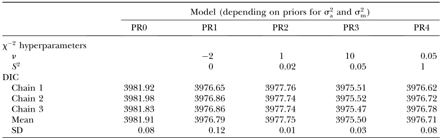
Table 2 shows the hyperparameters of the scaledx2 -priors (n and S2) tested for s2
a and s2m. The values chosen for these hyperparameters generated a wide range of shapes for this distribution that reflected differenta prioriknowledge on the expected values of both variance components. Model fit and complexity were evaluated with the DIC (Spiegelhalter et al.
2002), and PR3 was favored (DIC¼3975.50) although the difference was slight with respect to PR1 and PR4 (DIC¼3976.79 and 3976.71, respectively; Table 2). PR2 was penalized with a 2-units greater DIC than PR3, and the model without genetic effects (PR0) was discarded (DIC¼3981.91). Note that differences in DIC.3 are generally considered as statistically relevant (Burnham
and Anderson 1998; Spiegelhalter et al. 2002),
whereas lower discrepancies do not provide a strong evidence of a better fit and a lower degree of model complexity for a given comparison. It is important to highlight that three different MCMC chains were launched for each model and DIC showed a very small variance within models (Table 2).
As shown in Table 3, PR1, PR3, and PR4 models provided very similar estimates of variance components and their ratios, whereas PR2 had a lower value ofs2
a. Taking the PR3 model as reference and after correcting for systematic effects (generation and parturition num-ber of the female), the most important source of variation was that due to the uncontrolled factors that accounted fors2
e, its mode being 3.842 pups
2(Table 3).
TABLE 2
x2hyperparameter specifications and deviance information criterion (DIC) estimates
Model (depending on priors fors2 aands
2 m)
PR0 PR1 PR2 PR3 PR4
x2hyperparameters
n 2 1 10 0.05
S2 0 0.02 0.05 1
DIC
Chain 1 3981.92 3976.65 3977.76 3975.51 3976.62
Chain 2 3981.98 3976.86 3977.74 3975.52 3976.72
Chain 3 3981.83 3976.86 3977.74 3975.47 3976.78
Mean 3981.91 3976.79 3977.75 3975.50 3976.71
Nevertheless, genetic variancess2
aands2mwere high for an inbred strain, 0.151 and 0.035, respectively. It is important to note that the highest posterior density region at 95% (HPD95) for both variance components was away from zero, starting at 0.066 and 0.017, re-spectively (Table 3). Mutational heritability was 0.008, and the overall heritability at generation G1 (hG1
2 ¼
ðs2 a1s
2 mÞ=ðs
2 a1s
2 m1s
2 p11s
2 p21s
2
eÞ) was 0.045 (HPD95 between 0.010 and 0.062), showing that enough addi-tive genetic variance was available to develop a genetic trend under selection or drift. In a similar way, sire and (nongenetic) dam effects had moderate variance com-ponents (0.092 and 0.037, respectively), although with wide HPD95 (Table 3).
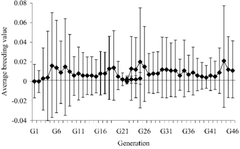
The C57BL/6J strain did not show notable genetic drift during 46 generations. The within-generation av-erage breeding value (a1m) ranged between 0 (G1, G2, and G22) and 0.02 pups (G44), with all the HPD95 including the null value (Figure 2). Similarly, within-generation average values for environmental effect (p1 andp2) did not differ from zero. The between-generations phenotypic variability was mainly accounted for by the generation number effects (results not shown). Model fit was worse when this systematic effect was dropped out (DIC¼4018.89).
The within-generations2
aðtÞquickly decreased (Figure
3) whereas the new genetic variance originated by mutation increased up to0.20 and oscillated around 0.15 thereafter (Figure 4). More specifically,s2
aðtÞstarted
with a modal estimate of 0.159 in generation G1(HPD95 between 0.056 and 0.245) and fell to values ,0.01 in ,10 generations. Mutational variance accumulated during the first generations and reached its maximum at generation G14(0.231), although it showed an oscil-lating pattern around 0.15 from generation G7(HPD95 reached values up to 0.400).
DISCUSSION
Prior distributions and Bayesian analysis:The mixed-model analysis of litter size in C57BL/6J mice was carried out using Bayesian methods. An important characteris-tic of the Bayesian analysis is that the final inference is based on the posterior distribution, resulting from combining two different sources of information. One of these sources is the experimental data, which are not influenced by arbitrary choices other than the model used for analysis. The other source of information is the assignment of prior distributions, which are arbitrarily chosen from previous knowledge of the parameters of TABLE 3
Modal estimates (and highest posterior density region at 95%) for the variance components and heritabilities
Model (depending on priors fors2 a ands
2 m)
PR0 PR1 PR2 PR3 PR4
s2
a 0.155 (0.067–0.260) 0.020 (0.000–0.103) 0.151 (0.066–0.254) 0.158 (0.070–0.273)
s2
m 0.033 (0.015–0.048) 0.025 (0.009–0.043) 0.035 (0.017–0.049) 0.035 (0.019–0.050)
s2
p1 0.112 (0.011–0.683) 0.105 (0.006–0.650) 0.099 (0.005–0.630) 0.092 (0.003–0.604) 0.099 (0.005–0.634) s2
p2 0.051 (0.009–0.612) 0.038 (0.006–0.555) 0.040 (0.008–0.602) 0.037 (0.002–0.596) 0.037 (0.003–0.606) s2
e 3.901 (3.332–4.054) 3.887 (3.326–4.003) 3.965 (3.376–4.101) 3.842 (3.245–3.991) 3.880 (3.322–3.995)
h2
m 0.008 (0.003–0.012) 0.006 (0.002–0.009) 0.008 (0.004–0.012) 0.008 (0.004–0.011)
h2
G1 0.045 (0.011–0.064) 0.011 (0.002–0.046) 0.045 (0.010–0.062) 0.046 (0.013–0.068)
h2 m¼s
2 m=ðs
2 a1s
2 m1s
2 p11s
2 p21s
2 eÞ;h
2 G1 ¼ ðs
2 a1s
2 mÞ=ðs
2 a1s
2 m1s
2 p11s
2 p21s
2 eÞ.
Figure2.—Mode (solid diamonds) and highest posterior density region at 95% (whiskers) of the average breeding value per generation.
Figure3.—Mode (solid diamonds) and highest posterior density region (whiskers) of the within-generation additive ge-netic variance (s2
interest. If previous information is not available, prior distributions become a blind choice and they could have a substantial impact on the posterior inference (Gianola
and Fernando 1986; Blasco 2001). Genetic
compo-nents of litter size in highly inbred mice have not been previously analyzed and we lacked accurate information on the expected values ofs2
aands 2
m. To assess influences of priors for both variance components, the analyses performed here made use of very different prior distri-butions fors2
aands 2
m, covering the range of mutational heritabilities reviewed by Lynch(1988) and Houleet al.
(1996) in other traits and species. Model PR0, the one without genetic components, showed the poorest model fit and DIC substantially decreased whens2
aands2mwere included in the model. This provided statistical evidence of the presence of additive genetic variance in this inbred strain. Models PR1–PR4 showed a similar fit, although the stringent prior fors2
a ands 2
m in model PR2 was mod-erately penalized. It is important to note that posterior inferences from models PR1, PR3, and PR4 did not differ substantially (Table 3). This reassuring conclusion in-dicated that the experimental data had enough informa-tion content to override moderate influences of prior information, and the model performed better under a vague assumption for s2
a and s 2
m over the parameter space.
Note that this analysis could also be performed under a frequentist approach by maximizing the likelihood function through iterative algorithms. These frequentist methods produce inferences based on the data and the previous knowledge of the distribution of estimators in the sampling space, without using prior information. As highlighted by Blasco(2001), the distribution of the
estimator is used for inferences instead of the distribu-tion of the parameter, which leads to a rather unnatural form of expressing uncertainly about the results of an experiment. Within the Bayesian context, conceptual simplicity is gained because inferences are made from probabilities associated with values of the parameter of interest.
Genetic variability: Reported estimates of mutational heritability found in the literature commonly range be-tween 104 and 53102 (Lynch 1988; Houle et al.
1996), although this parameter has never been estimated for litter size in mice. Our estimate fell within this interval (0.008; Table 3) and was very close to the values reported by Keightleyand Hill(1992) and Keightley(1998)
for body size in mice. Although Wray’s (1990) approach
assumes that mutations are small and additive, the inclusion of sire and dam environmental effects ac-counted for deviations from the infinitesimal model, allowing for a more accurate estimation ofs2
m. Within this context, part of the variability that accounted fors2
p1and s2
p2could have originated from large mutations. Thus,s2m likely underestimates all the genetic variation originated by mutation. Moreover, environmental variance could also account for nonadditive genetic mutations (Zhang et al. 2004). Althoughs2
p1 ands 2
p2 modal estimates sug-gested a greater impact ofs2
p1on litter size, HPD95 were completely overlapping. It is important to note thataand m accounted for additive genetic effects whereas non-additive genetic sources of variation such as inbreeding or heterosis could have a substantial impact on mouse litter size (Bhuvanakumaret al. 1985; Hinrichset al. 2007).
Given the difficulty in accommodating inbreeding and heterosis on the new mutational variability originated at each generation, as well as other nonadditive genetic ef-fects (i.e., epistasis or dominance), we restricted the model to pure additive genetic effects and assumed that the re-maining nonadditive genetic influences were accounted for byp1andp2or were absorbed by the residual term. Mutation variance in the mixed model was modeled as the dispersion term associated with random mutation effects arising in each offspring (Wray 1990). This
parameterization has been typically used in mutation experiments (Lynch 1988; Houle et al. 1996) and
describes the potential effect of mutations in a very short time interval. Nevertheless, new mutations accumulate in successive generations, sometimes fixed or removed due to selection or genetic drift, ands2
m must be viewed in highly inbred strains as a lower limit of the accumulated (mutation) genetic variance. As shown in Figure 4, the within-generation mutation variance increased with gen-eration, up to G14. This is in agreement with a continuous input of new mutations with effects on litter size. The oscillating pattern around 0.15 after G14agrees withs2a 1ð Þ
at G1and suggests an equilibrium between new muta-tions and the fixation or loss of mutamuta-tions due to genetic drift and inbred matings. In a similar way,s2
alacks addi-tional sources of new variation and its within-generation estimates have a rapid decrease after a few generations, which is related to the small population size and the mating system. Both within-generation s2
a ands 2 m esti-mates support the conclusion that this C57BL/6J strain maintained a substantial degree of genetic variance across generations, accounting for an overall heritability around 0.05 (Table 3). This value is clearly lower than the Figure4.—Mode (solid diamonds) and highest posterior
density region (whiskers) of the within-generation mutational variance (s2
ones reported in outbred mouse populations (0.15–0.33; Falconer1960; Joakimsenand Baker1977; Longet al.
1991) although it indicates a substantial and generally unaccounted for degree of genetic variability in an in-bred strain.
Absence of environmental and genetic trend across generations:Mice bred under inbred mating systems for prolonged periods should fix the vast majority (poten-tially all) of the genetic contribution to variation (Bailey1982) and typically, individual mice within an
inbred strain are considered genetically identical. Nev-ertheless, unexpected genetic variability has been ob-served in highly inbred mouse strains (Keightleyand
Hill 1992), even allowing for genetic drift (Bailey
1977) and genetic trend on phenotypic traits (Festing
1973; Keightley1998). Indeed, incongruities between
genetic homogeneity and phenotypic variability were first recognized.40 years ago (Wolff1961) and this
issue is an area of concern in laboratory species. The C57BL/6J strain was developed in the early 20th century from a very small founder population and it is consid-ered a classical inbred strain with an almost homozygous genome (Wadeand Daly2005). As reported in other
inbred mouse strains (Falconer1960), our strain showed
substantial phenotypic variation for average litter size across generations, average litter size being similar to the estimates reported by other authors (Kirkpatrick et al. 1998; Corvaet al. 2004). Note that this population
was not under selection for litter size.
Besides the continuous generation of additional ge-netic variability in our C57BL/6J population, gege-netic drift did not take place (Figure 2) and changes in the (within-generation) average environmental effect were also negligible. As mentioned above, our mixed-model analysis included generation number as a systematic effect and it accounted for the major differences between generations in litter size. Note that model fit was worse when this effect was dropped out (DIC¼4018.89). The-oretically, this effect must be viewed as the generation-specific contribution of multiple environmental sources of variation (e.g., food, housing, and management among others) although some genetic contributions could be involved too. Additive genetic variability is accounted for byaandm, and residual effects can absorb (individual-specific) nonadditive genetic influences. Nevertheless, a small number of breeding individuals contribute to the next generation and commonly they are closely related (full sibs in the majority of cases). Nonadditive genetic effects from a given ancestor can be widely spread in the following generation, reducing between-individuals variability and therefore being partially accounted for by the within-generation overall mean (generation number effect). Within this context, ge-netic drift cannot be completely discarded although, if present, it would be due to nonadditive mutations.
In conclusion, we present a new approach to Wray’s
(1990) method for modeling s2
a and s2m within a
Bayesian framework, where all parameters in the mixed model can be inferred using the Gibbs sampling algorithm. The analysis of litter size in the C57BL/6J strain indicated a low mutational input of genetic variance per generation (s2
m ¼ 0.035), although the accumulation of new mutations in successive genera-tions led to a substantial amount of additive genetic variability (h2¼0:045). While genetic uniformity of highly inbred strains is a key point in several research areas (Stevenset al. 2007), our estimates do not support
this assumption and confirm a continuous and unavoid-able flow of new genetic variability. These results contribute to the understanding of mutation–drift equilibrium in experimental populations.
We are appreciative of the excellent efforts of Vince De Vera in mouse husbandry and phenotypic data collection. The useful com-ments of D. Gianola and an anonymous referee are greatly appreci-ated. This research was supported by the National Research Initiative grant no. 2005-35205-15453 from the U.S. Department of Agriculture Cooperative State Research, Education, and Extension Service and by the California Agricultural Experimental Station. The research contract of J. Casellas was partially financed by Spain’s Ministerio de Educacio´n y Ciencia (program Juan de la Cierva).
LITERATURE CITED
Bailey, D. W., 1977 Sources of subline divergence and their relative
importance for sublines of six major inbred strains of mice, pp. 197–215 inOrigins of Inbred Mice, edited by H. C. Morse.
Aca-demic Press, New York.
Bailey, D. W., 1982 How pure are inbred strains of mice? Immunol.
Today3:210–214.
Bhuvanakumar, C. K., R. C. Roberts and W. G. Hill,
1985 Heterosis among lines of mice selected for body weight. Theor. Appl. Genet.71:52–56.
Blasco, A., 2001 The Bayesian controversy in animal breeding. J.
Anim. Sci.79:2023–2046.
Blasco, A., D. Sorensenand J. P. Bidanel, 1998 Bayesian inference
of genetic parameters and selection response for litter size com-ponents in pigs. Genetics149:301–306.
Bradford, G. E., and T. R. Famula, 1984 Evidence for a major
gene for rapid postweaning growth in mice. Genet. Res. 44:
293–298.
Burnham, K. P., and D. R. Anderson, 1998 Model Selection and Inference. A Practical Information Theoretic Approach.Springer-Verlag, New York. Caballero, A., M. A. Toroand C. Lo´ pez-Fanjul, 1991 The
re-sponse to artificial selection from new mutations inDrosophila mel-anogaster.Genetics127:89–102.
Corva, P. M., N. C. Mucci, K. Evansand J. F. Medrano, 2004 Diet
effects on female reproduction in high growth (hg/hg) mice that are deficient in theSocs-2gene. Reprod. Nutr. Dev.44:303–312. Falconer, D. S., 1960 The genetics of litter size in mice. J. Cell.
Comp. Physiol.56(Suppl. 1): 153–167.
Festing, M., 1973 A multivariate analysis of subline divergence in
the shape of the mandible in C57BL/Gr mice. Genet. Res.21:
121–132.
Fisher, R. A., 1918 The correlation between relatives under the
supposition of Mendelian inheritance. Trans. R. Soc. Edinb.52:
399–433.
Gianola, D., and R. L. Fernando, 1986 Bayesian methods in animal
breeding theory. J. Anim. Sci.63:217–244.
Gianola, D., R. L. Fernando, S. Imand J. L. Foulley, 1989
Like-lihood estimation of quantitative genetic parameters when selec-tion occurs: models and problems. Genome31:768–777. Gilks, W. R., S. Richardsonand D. J. Spiegelhalter, 1996
Intro-ducing Markov chain Monte Carlo, pp. 1–19 in Markov Chain Monte Carlo in Practice, edited by W. R. Gilks, S. Richardson
Henderson, C. R., 1973 Sire evaluations and genetic trends, pp. 10–
41 inProceedings of the Animal Breeding and Genetics Symposium in Honor of Dr. Jay L. Lush. American Society of Animal Science and American Dairy Science Association, Champaign, IL. Hill, W. G., 1982a Rates of change in quantitative traits from
fixa-tion of new mutafixa-tions. Proc. Natl. Acad. Sci. USA79:142–145. Hill, W. G., 1982b Predictions of response to artificial selection
from new mutations. Genet. Res.40:255–278.
Hill, W. G., 2007 A century of corn selection. Science307:683–684.
Hinrichs, D., T. H. E. Meuwissen, J. Ødegard, M. Holt, O. Vangen et al., 2007 Analysis of inbreeding depression in the first litter size of mice in a long-term selection experiment with respect to the age of the inbreeding. Heredity99:81–88.
Houle, D., B. Morikawaand M. Lynch, 1996 Comparing
muta-tional variabilities. Genetics143:1467–1483.
Im, S., R. L. Fernandoand D. Gianola, 1989 Likelihood inferences
from animal breeding data subject to selection. Genet. Sel. Evol.
21:399–414.
Joakimsen, O., and R. L. Baker, 1977 Selection for litter size in
mice. Acta Agric. Scand.27:301–318.
Keightley, P. D., 1998 Genetic basis of response to 50 generations
of selection on body weight in inbred mice. Genetics148:1931– 1939.
Keightley, P. D., and W. G. Hill, 1992 Quantitative genetic variation
in body size of mice from new mutations. Genetics131:693–700. Kirkpatrick, B. W., J. A. Ariasand J. J. Rutledge, 1988 Effects of
prenatal and postnatal fraternity size on long-term reproduction in mice. J. Anim. Sci.66:62–69.
Kirkpatrick, B. W., A. Mengelt, N. Schulmanand I. C. A. Martin,
1998 Identification of quantitative trait loci for prolificacy and growth in mice. Mamm. Genome9:97–102.
Long, C. R., W. R. Lambersonand R. O. Bates, 1991 Genetic
cor-relations among reproductive traits and uterine dimensions in mice. J. Anim. Sci.69:99–103.
Lynch, M., 1988 The rate of polygenic mutation. Genet. Res.51:
137–148.
Macarthur, J. W., 1949 Selection for small and large mice in the
house mouse. Genetics34:194–209.
Mackay, T. F. C., J. D. Fry, R. F. Lymanand S. V. Nuzhdin, 1994
Poly-genic mutation inDrosophila melanogaster: estimates from response to selection of inbred strains. Genetics136:937–951.
Quaas, R. L., 1976 Computing the diagonal elements and inverse of
a large numerator relationship matrix. Biometrics32:949–953. Raftery, A. E., and S. M. Lewis, 1992 How many iterations in the
Gibbs sampler?, pp. 763–773 inBayesian Statistics IV, edited by J. M. Bernardo, J. O. Berger, A. P. Dawidand A. F. M. Smith.
Ox-ford University Press, OxOx-ford.
Schilling, P., W. Northand R. Bogart, 1968 The effect of sire on
litter size in mice. J. Hered.59:351–352.
Sorensen, D., R. Fernandoand D. Gianola, 2001 Inferring the
tra-jectory of genetic variance in the course of artificial selection. Genet. Res. Camb.77:83–94.
Sorensen, D. A., C. S. Wang, J. Jensen and D. Gianola,
1994 Bayesian analysis of genetic change due to selection using Gibbs sampling. Genet. Sel. Evol.26:333–360.
Spiegelhalter, D. J., N. G. Best, B. P. Carlinand A.van derLinde,
2002 Bayesian measures of model complexity and fit. J. R. Stat. Soc. B64:583–639.
Stevens, J. C., G. T. Banks, M. F. W. Festingand E. M. C. Fisher,
2007 Quiet mutations in inbred strains of mice. Trends Mol. Med.13:512–519.
Taft, R. A., M. Davissonand M. V. Wiles, 2006 Know thy mouse.
Trends Genet.22:649–653.
Wade, C. M., and M. J. Daly, 2005 Genetic variation in laboratory
mice. Nat. Genet.37:1175–1180.
Wolff, G. L., 1961 Some genetic aspects of physiological variability.
Cancer Res.21:1119–1123.
Wray, N. R., 1990 Accounting for mutation effects in the additive
genetic variance-covariance matrix and its inverse. Biometrics
46:177–186.
Wright, S, 1922 Coefficients of inbreeding and relationship. Am.
Nat.56:330–338.
Yoo, B. H., 1980 Long-term selection for a quantitative character in
large replicate populations ofDrosophila melanogaster.II. Lethal and visible mutants with large effects. Genet. Res.35:19–31.
Zhang, X., J. Wangand W. G. Hill, 2004 Influence of dominance,
leptokurtosis and pleitotropy of deleterious mutations on quan-titative genetic variation at mutation-selection balance. Genetics
166:597–610.
Communicating editor: R. W. Doerge
APPENDIX
Following in part Wray(1990), the additive genetic
(co)variance matrix including mutation effects can be partitioned as
A0s2a1Ms 2
m¼A0s2a1
Xt
k¼0 Aks2m;
where t is the number of generations, Ak is the full relationship matrix of additive genetic effects attributed to mutations arising in time unit (or generation)k, and A0 is the full relationship matrix including all individ-uals in the pedigree. For the mixed-model equations, both A1
0 and M
1 are required, computational effi-ciency becoming a key point. As developed by Quaas
(1976),A01 can be recursively computed from a list of individual sire and dam identifications ordered by age of individuals. Following in part Wray(1990),M1can
also be computed from an age-ordered pedigree withn
individuals and three vectors, u, v, and h, all with dimensionn31. Computation efficiency is gained with
n rounds, with the following calculations in the ith round,
vi¼
ffiffiffiffiffiffiffiffiffiffiffiffiffiffiffiffiffiffiffiffiffiffiffiffiffiffiffiffiffiffiffiffiffiffiffiffi
up1uq
4
hp1hq
2 11 q
both parents ofiare knownðpandqÞ ffiffiffiffiffiffiffiffiffiffiffiffiffiffiffiffiffiffiffiffi
uq
4
hq
21 1 2 q
only one parent ofiis knownðqÞ
1 neither parent ofiis known;
8 > > > > > < > > > > > :
wherevl,ul, andhlare thelth elements in vectorsv,u, andh, respectively. Forj¼i11;. . .;n,
vj¼
vpi1vqi
2 ifi # pj,qj
vpi
2 ifpj,i#qj 0 ifpj#qj,i; 8
> > < > > :
where pj and qj are parents of thejth individual and pj,qj. Forj ¼i11; . . . ;n,
hj ¼
hj1 vpjvqj
2 ifi#pj,qj
hj ifpj,i (
and forj ¼i;. . .;n,
uj ¼uj1vj2:
vi2tomii
vi2=2 tomip;mpi;miq;andmqi vi2=4 tompp;mpq;mqp;andmqq;
where mkl is the element in the kth row and lth column ofM1.
b. If only one parent ofiis known (q), add
vi2tomii
vi2=2 tomiqandmqi vi2=4 tomqq:
c. If neither parent ofiis known, add
vi2tomii:
Note that this construction ofA1 0 andM
1allows for a separate inference of additive genetic effects in the base population and new mutations arising in successive generations,A1
0 andM
1being independent from the remaining parameters in the model. If Bayesian mixed models are applied, this parameterization leads to well-known conditional posterior distributions for all param-eters, allowing for standard Gibbs sampling. On the contrary, conditional posterior distributions for several parameters under the original Wray’s (1990) approach