Uncertainty Quantification in Nuclear Reactor Modeling using Stochastic Sampling with the Virtual Environment for Reactor Applications.

ABSTRACT

SEDOTA, CHRISTOPHER STEPHEN. Uncertainty Quantification in Nuclear Reactor Modeling using Stochastic Sampling with the Virtual Environment for Reactor Applications. (Under the direction of Scott Palmtag.)

Uncertainty quantification is an important component of model development. In uncertainty

quantification, uncertainties in the inputs to a model are propagated through the model, and the resulting uncertainty in the model output is analyzed. The various methods for uncertainty

quantification can be divided into two classes: statistical methods and deterministic methods.

Stochastic sampling, a statistical method, is exclusively used in this study. The model is the Virtual Environment for Reactor Applications (VERA). The uncertain inputs to the model are the multigroup

cross sections and fuel rod manufacturing parameters. One thousand perturbed multigroup cross

section libraries were generated. These perturbed cross section libraries were used with a variety of benchmark problems based on the Three Mile Island Unit 1 Pressurized Water Reactor, the Peach

Bottom Unit 2 Boiling Water Reactor, and the Watts Bar Unit 1 Pressurized Water Reactor. When

only considering the uncertainty in the effective neutron multiplication factor due to cross section uncertainty, the relative standard deviation for all cases was determined to be approximately 0.5 –

0.6 %.

In this study, one thousand perturbed cross section libraries were used for stochastic sampling. A major question that this study aims to address is whether one thousand cross section libraries

is sufficient for quantification of cross section uncertainty using stochastic sampling, or whether

fewer libraries could be used. The use of more or fewer cross section libraries has major implications on computational cost, particularly for very large cases. For all cases that were examined, the

estimated relative standard error of the standard deviation estimate was approximately 2 % when

one thousand cross section libraries were used. The use of 500 cross section libraries, which is a reduction of computational cost of 50 %, increased the relative standard error to approximately

3 % for all cases. Even when only 250 cross section libraries were used, which is a 75 % reduction in

computational cost from the full one thousand libraries, the relative standard error of the standard deviation estimate remained below 5 % for all cases. Therefore it was determined that with

well-sampled cross sections, fewer than the full one thousand cross section libraries could be used to generate valid uncertainty results.

Uncertainty in the dimensions and composition of the fuel rods was also quantified. The VERA

format of individual pin specification facilitated this analysis, and a tool was developed to perform material parameter perturbations on a base VERA input deck. It was found that the size of the

problem had a significant impact on the uncertainty due to material parameter uncertainties. For

instance, while the estimated relative standard deviation of the effective neutron multiplication factor for the Three Mile Island Unit 1 pincell was 0.07 %, the relative standard deviation for the

Three Mile Island Unit 1 lattice was 0.007 %, a factor of 10 lower. The effect of the exact application

© Copyright 2020 by Christopher Stephen Sedota

Uncertainty Quantification in Nuclear Reactor Modeling using Stochastic Sampling with the Virtual Environment for Reactor Applications

by

Christopher Stephen Sedota

A thesis submitted to the Graduate Faculty of North Carolina State University

in partial fulfillment of the requirements for the Degree of

Master of Science

Nuclear Engineering

Raleigh, North Carolina

2020

APPROVED BY:

Jason Hou Ralph Smith

Scott Palmtag

DEDICATION

BIOGRAPHY

Chris Sedota was born in Rochester, NY and grew up in Mooresville, NC. He attended Lake Norman High School, where a number of passionate science and mathematics teachers influenced him to

pursue engineering in higher education. He attended North Carolina State University and obtained

ACKNOWLEDGEMENTS

I would like to thank my advisor, Dr. Scott Palmtag, for his immense help in the completion of this thesis. I would also like to thank Dr. Jason Hou and Dr. Ralph Smith, who agreed to serve on my

graduate committee, and all the great educators who helped me along the way. Finally, I would like

to thank Dr. Matt Jessee and Dr. Kang Seog Kim for generating the perturbed cross section libraries used in this study.

This research was supported by the Consortium for Advanced Simulation of Light Water Reactors

(http://www.casl.gov), an Energy Innovation Hub (http://www.energy.gov/hubs) for Modeling and Simulation of Nuclear Reactors under U.S. Department of Energy Contract No. DE-AC05-00OR22725.

This research also made use of the resources of the High Performance Computing Center at Idaho National Laboratory, which is supported by the Office of Nuclear Energy of the U.S. Department of

TABLE OF CONTENTS

LIST OF TABLES . . . vii

LIST OF FIGURES. . . ix

Chapter 1 INTRODUCTION . . . 1

1.1 Motivation . . . 2

1.2 Classes of Uncertainty Quantification . . . 3

1.2.1 Uncertainty Quantification using Deterministic Methods . . . 3

1.2.2 Uncertainty Quantification using Stochastic Sampling . . . 6

1.2.3 Comparison of Methods . . . 7

1.3 Neutron Multiplication Factor . . . 9

1.4 Cross Section Uncertainty . . . 10

1.5 Material Uncertainty . . . 11

1.6 Benchmark Problem Naming Convention . . . 11

1.7 Research Objectives . . . 12

1.8 Thesis Layout . . . 12

Chapter 2 METHODOLOGY . . . 14

2.1 SCALE . . . 14

2.2 MPACT . . . 15

2.2.1 Resonance Self-Shielding . . . 17

2.3 Computational Cost . . . 17

2.4 Material Perturbation Mechanism . . . 19

Chapter 3 BENCHMARK CROSS SECTION UNCERTAINTY . . . 26

3.1 Benchmark Configuration . . . 26

3.1.1 PWR Pincell . . . 27

3.1.2 PWR Lattice . . . 29

3.1.3 PWR Colorset . . . 29

3.1.4 BWR Pincell . . . 31

3.1.5 BWR Lattice . . . 31

3.2 Benchmark Results . . . 35

3.2.1 Comparison to Benchmark Averages . . . 37

Chapter 4 WATTS BAR CROSS SECTION UNCERTAINTY . . . 40

4.1 Watts Bar Configuration . . . 40

4.2 2D Watts Bar . . . 42

4.3 3D Watts Bar . . . 43

4.4 3D Watts Bar with Thermal Hydraulic Feedback . . . 44

4.5 3D Watts Bar Full-Core Depletion . . . 46

4.6 Comparison of Cases . . . 47

Chapter 5 SAMPLE SIZE . . . 49

5.1 Standard Error of Estimators . . . 49

5.1.1 Standard Error of the Mean . . . 51

5.2 Jackknife Resampling as a Technique to Estimate Standard Errors of Parameters . . . . 53

5.3 Jackknife Estimates of Standard Error of Standard Deviation Estimate for Benchmark Cases . . . 53

5.4 Jackknife Estimates of Standard Error of Standard Deviation Estimate for Watts Bar Cases . . . 59

5.5 Standard Error of Standard Deviation Estimate for Watts Bar Unit 1 Full-Core Depletion 61 Chapter 6 MATERIAL UNCERTAINTY . . . 63

6.1 Sources of Material Uncertainty . . . 64

6.2 PWR Pincell . . . 65

6.3 PWR Lattice . . . 68

Chapter 7 Conclusions . . . 73

7.1 Suggestion for Future Work . . . 75

BIBLIOGRAPHY . . . 81

APPENDIX . . . 83

Appendix A Confidence Intervals . . . 84

A.1 Theory . . . 84

LIST OF TABLES

Table 1.1 Pros and cons of deterministic and stochastic sampling methods for

uncer-tainty quantification. . . 9

Table 1.2 UAM LWR benchmark problem naming convention. . . 11

Table 2.1 Profiling data for UAM LWR benchmark cases. . . 18

Table 2.2 Profiling data for Watts Bar Unit 1 full-core cases. . . 19

Table 3.1 State parameters for the UAM LWRs. . . 27

Table 3.2 PWR pincell parameters[Iva13]. . . 28

Table 3.3 PWR lattice parameters[Iva13]. . . 30

Table 3.4 BWR pincell parameters[Iva13]. . . 31

Table 3.5 BWR rod types[Iva13]. . . 32

Table 3.6 BWR lattice parameters[Iva13]. . . 34

Table 3.7 BWR control blade parameters[Iva13]. . . 35

Table 3.8 Mean and standard deviation of k-eff. . . 36

Table 3.9 Comparison of results with benchmark average (B.A.) results. . . 37

Table 3.10 Absolute differences in obtained results with respect to benchmark average results. . . 38

Table 3.11 Comparison of standard deviation (SD) with benchmark average (B.A.) stan-dard deviation. . . 39

Table 4.1 Watts Bar pin parameters[God14]. . . 41

Table 4.2 Watts Bar and UAM LWR lattice parameters[God14] [Iva13]. . . 41

Table 4.3 Estimated Mean and Standard Deviation for Watts Bar Cases. . . 48

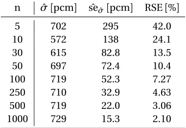
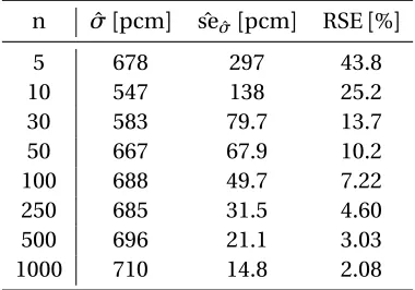
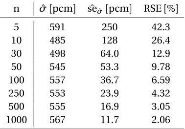
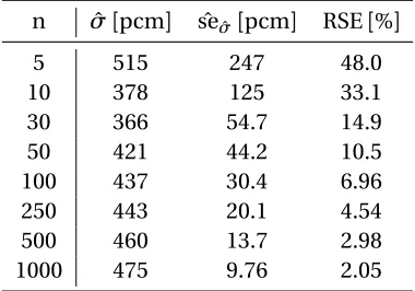
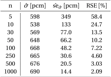
Table 5.1 Reduction of standard error of standard deviation estimate with increasing sample size, PWR Pincell at HZP (PPZ). . . 54

Table 5.2 Reduction of standard error of standard deviation estimate with increasing sample size, PWR Pincell at HFP (PPF). . . 54

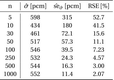
Table 5.3 Reduction of standard error of standard deviation estimate with increasing sample size, BWR Pincell at HZP (BPZ). . . 55

Table 5.4 Reduction of standard error of standard deviation estimate with increasing sample size, BWR Pincell at HFP (BPF). . . 55

Table 5.5 Reduction of standard error of standard deviation estimate with increasing sample size, Unrodded PWR Lattice at HZP (PLUZ). . . 55

Table 5.6 Reduction of standard error of standard deviation estimate with increasing sample size, Unrodded PWR Lattice at HFP (PLUF). . . 56

Table 5.7 Reduction of standard error of standard deviation estimate with increasing sample size, Rodded PWR Lattice at HZP (PLRZ). . . 56

Table 5.8 Reduction of standard error of standard deviation estimate with increasing sample size, Rodded PWR Lattice at HFP (PLRF). . . 56

Table 5.9 Reduction of standard error of standard deviation estimate with increasing sample size, Unrodded BWR Lattice at HZP (BLUZ). . . 57

Table 5.11 Reduction of standard error of standard deviation estimate with increasing

sample size, Rodded BWR Lattice at HZP (BLRZ). . . 57

Table 5.12 Reduction of standard error of standard deviation estimate with increasing sample size, Rodded BWR Lattice at HFP (BLRF). . . 58

Table 5.13 Reduction of standard error of standard deviation estimate with increasing sample size, PWR Colorset at HZP (PCZ). . . 58

Table 5.14 Reduction of standard error of standard deviation estimate with increasing sample size, PWR Colorset at HFP (PCF). . . 58

Table 5.15 Reduction of standard error of standard deviation estimate with increasing sample size, 2D Watts Bar full-core. . . 59

Table 5.16 Reduction of standard error of standard deviation estimate with increasing sample size, 3D Watts Bar full-core. . . 60

Table 5.17 Reduction of standard error of standard deviation estimate with increasing sample size, 3D Watts Bar full-core with thermal hydraulic feedback. . . 60

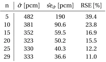
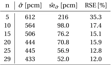
Table 5.18 Reduction of standard error of standard deviation estimate with increasing sample size, Watts Bar full-core at BOC. . . 61

Table 5.19 Reduction of standard error of standard deviation estimate with increasing sample size, Watts Bar full-core at MOC. . . 62

Table 5.20 Reduction of standard error of standard deviation estimate with increasing sample size, Watts Bar full-core at EOC. . . 62

Table 6.1 Material Parameter Uncertainties for the PWR[Iva13]. . . 65

Table 6.2 Material Parameter Uncertainties for the PWR Pincell at HZP. . . 66

Table 6.3 Material Parameter Uncertainties for the unrodded PWR lattice at HZP. . . 72

Table 7.1 Comparison between simplest and most complex case for each model. . . 76

LIST OF FIGURES

Figure 1.1 Stochastic sampling flow chart. . . 6

Figure 1.2 VERA code structure[CAS18]. . . 8

Figure 2.1 Characteristics imposed on a pincell[Col16]. . . 16

Figure 2.2 Sample input deck for PWR Lattice with material parameter uncertainty. . . . 25

Figure 3.1 Two-dimensional pincell geometry. The pitch in Table 3.2 corresponds to the side length of the black boundary. . . 28

Figure 3.2 PWR lattice configuration. . . 29

Figure 3.3 PWR colorset configuration. Each square corresponds to one assembly. . . 30

Figure 3.4 BWR lattice configuration with rod type labels. . . 32

Figure 3.5 BWR axial configuration. . . 33

Figure 3.6 BWR assembly diagram. Labels correspond to Table 3.6. . . 34

Figure 3.7 BWR control blade structure. Labels correspond to Table 3.7. . . 35

Figure 4.1 Watts Bar loading pattern[God14]. . . 42

Figure 4.2 Two-dimensional Watts Bar k-eff distribution. . . 43

Figure 4.3 Three-dimensional Watts Bar k-eff distribution. . . 44

Figure 4.4 Watts Bar with thermal hydraulic feedback k-eff distribution. . . 46

Figure 4.5 Critical boron concentration as a function of exposure, full-core Watts Bar. . 47

Figure 6.1 Kernel density estimate of the k-eff distributions when varying each material parameter individually. . . 67

Figure 6.2 Kernel density estimate of the k-eff distributions when varying each material parameter individually, 10x fuel enrichment uncertainty. . . 68

Figure 6.3 k-eff distribution for PWR Lattice Unrodded at HZP, varying all material parameters on a pin-level. . . 69

Figure 6.4 k-eff distribution for PWR Lattice Unrodded at HZP, varying all material parameters on a pin-level and varying cross sections. . . 70

Figure 6.5 k-eff distribution for PWR Lattice Unrodded at HZP, varying fuel composition parameters on an assembly-level. . . 70

Figure 6.6 k-eff distribution for PWR Lattice Unrodded at HZP, varying fuel composition parameters on an assembly-level with cross sections. . . 71

Figure 7.1 Confidence intervals for PWR Pincell and PWR Colorset models. . . 76

Figure 7.2 Confidence intervals through 50 samples for PWR Pincell and PWR Colorset models. . . 77

Figure 7.3 Relative standard deviations for the PWR pincell at HZP and the PWR colorset at HFP. . . 78

Figure 7.4 Relative standard deviation difference between the PWR pincell at HZP and the PWR colorset at HFP. . . 78

Figure 7.5 Relative standard deviations for the 2D Watts Bar model and the 3D Watts Bar full- core with thermal hydraulic feedback, N=200. . . 79

Figure 7.6 Relative standard deviations for the 2D Watts Bar model and the 3D Watts Bar full- core with thermal hydraulic feedback. . . 80

Figure A.2 PWR Pincell at HFP 95 % confidence interval. . . 87

Figure A.3 PWR Lattice Unrodded at HZP 95 % confidence interval. . . 87

Figure A.4 PWR Lattice Unrodded at HFP 95 % confidence interval. . . 88

Figure A.5 PWR Lattice Rodded at HZP 95 % confidence interval. . . 88

Figure A.6 PWR Lattice Rodded at HFP 95 % confidence interval. . . 89

Figure A.7 PWR Colorset at HZP 95 % confidence interval. . . 89

Figure A.8 PWR Colorset at HFP 95 % confidence interval. . . 90

Figure A.9 BWR Pincell at HZP 95 % confidence interval. . . 90

Figure A.10 BWR Pincell at HFP 95 % confidence interval. . . 91

Figure A.11 BWR Lattice Unrodded at HZP 95 % confidence interval. . . 91

Figure A.12 BWR Lattice Unrodded at HFP 95 % confidence interval. . . 92

Figure A.13 BWR Lattice Rodded at HZP 95 % confidence interval. . . 92

Figure A.14 BWR Lattice Rodded at HFP 95 % confidence interval. . . 93

Figure A.15 Watts Bar two-dimensional full core 95 % confidence interval. . . 93

Figure A.16 Watts Bar three-dimensional full core 95 % confidence interval. . . 94

CHAPTER

1

INTRODUCTION

Uncertainty quantification is a critical component of the analysis of any system. If there are

un-certainties in the inputs to a system, there will necessarily be uncertainty in the response of the system. Knowledge of the uncertainty in a system can help establish confidence in the system and

allow designers to make more informed decisions on the edge of the design space, which is where

efficient designs exist.

When dealing with any complex system, modeling and simulation is used to gain information of

the system in place of physical experimentation whenever possible. Certainly nuclear systems can

be characterized as complex systems. Consider the cost associated with physically testing a new fuel assembly design in an active power reactor. Neglecting even the initial cost to manufacture the

novel fuel assembly, which would likely exceed the estimated 1 million USD cost of manufacturing a

typical fuel assembly[Kok09], the cost associated with potentially reducing the power production of a commercial reactor for experimentation is very large. If the reactor needed to be taken off-line for

experimentation, it could cost the operators of the reactor upwards of 500,000 USD per day[Str95], which is the approximate cost typically associated with refueling outages.

The other alternative for physical experimentation in a power-producing reactor is the

construc-tion of dedicated experimental facilities. This is another extremely expensive opconstruc-tion. For instance, the Versatile Test Reactor (VTR) project, which is slated to begin construction at Idaho National

Lab-oratory in 2022, has an initial cost estimate of 3-6 billion USD[Ida]. While physical experimentation is an unavoidable and necessary component of gaining knowledge of a system, in many cases it is avoided as much as possible due to its extreme cost. Clearly it is in the interest of those associated

with nuclear power to use modeling and simulation in place of physical experimentation wherever

The high cost associated with physical experimentation has prompted the development of very

sophisticated models to model and predict reactor behavior. The modeling of light water reactors (LWRs) requires a wide range of physics to be considered, from the interaction of neutrons with

matter to the complex multi-phase flow of the water coolant through the core. The Consortium for

the Advanced Simulation of Light Water Reactors (CASL) was established by the US Department of Energy as a collaborative effort between universities, national laboratories, and industry participants

with the goal of improving the modeling of light water reactor modeling. To achieve this goal, a

high-fidelity reactor simulation suite called the Virtual Environment for Reactor Applications (VERA) was developed.

As VERA has matured into a production-level code system, increased interest has been placed on

using it as a model for uncertainty quantification. Uncertainty quantification is an activity that can only be undertaken when there is sufficient confidence in the underlying model. This confidence is

gained through rigorous solution and code verification, which ensures that errors are not present in

the coding implementation of the underlying mathematical model[Roy05], and validation exercises, where the predictive capability of the model is assessed against experimental data. The predictive

capability of VERA tools were largely tested using a series of progression problems based on the

Watts Bar Unit 1 reactor[God14], a few of which have associated physical data.

The governing equations of the neutronics component of nuclear systems have been relatively

well-understood from the inception of the field of nuclear engineering. The neutron transport equation, for instance, which accounts for the movement of neutrons about a system, was developed

in the 1940s[Dud76]. With the rapid advancement of computing since then, the neutron transport equation has been widely implemented in computer codes to model nuclear systems, and still provides the basis for neutronics codes today.

The neutronics component of VERA is the Michigan PArallel Characteristics based Transport

(MPACT) code[Koc17]. MPACT serves as the model for most of the uncertainty analysis in this study. MPACT coupled with the thermal hydraulic code CTF[Sal16]serves as the model for uncertainty analysis in a 3-dimensional Watts Bar Unit 1 system with thermal hydraulic feedback.

1.1

Motivation

With computational uncertainty quantification, the ultimate goal is to obtain high-quality

uncer-tainty information at a low computational cost. Unceruncer-tainty quantification can be used to reduce

conservative margins that have been built into reactor design. With little or no knowledge of the uncertainty of a system, generous margin must be included to ensure safety. If high-quality

uncer-tainty information is known, then this generous margin can be reduced while still ensuring safety. Reduction in margin often means more economical design and operation can be achieved.

As will be discussed in the following sections, there are significant computational cost differences

be given to two concepts that could reduce computational expense: the potential use of simpler

problems to serve as surrogate problems for more complex problems, and the number of samples necessary to produce reliable uncertainty information for different cases. Chapters 3 and 4 will

show how simple cases compare to more complex, and thus more computationally expensive, cases.

Chapter 5 deals with the latter consideration – the sample size required to generate high-quality uncertainty information for a wide range of cases.

1.2

Classes of Uncertainty Quantification

Uncertainty analysis can be broadly divided into two classes: stochastic methods and

determin-istic methods. Although stochastic methods are exclusively used in this study, it is beneficial to understand both classes, and the advantages and disadvantages that each method brings.

1.2.1 Uncertainty Quantification using Deterministic Methods The k-eigenvalue neutron transport problem[Lew93]is

_ˆ

Ω·∇~+Σ(~r,E)ψ ~r, ˆΩ,E− Z

d E0

Z

dΩ0Σs r~,E0→E, ˆΩ0·Ωˆ

ψ ~r, ˆΩ0,E0

=χ(E)

k

Z

d E0νΣf r~,E0

Z

dΩ0ψ ~r, ˆΩ0,E0, (1.1)

where

Σ(~r,E) =total macroscopic cross section at positionr~at energyE, ψ(~r, ˆΩ,E) =angular neutron flux at positionr~in direction ˆΩat energyE, Σs r~,E0→E, ˆΩ0·Ωˆ

=macroscopic scattering cross section at positionr~from energyE0toE

and from direction ˆΩ’ to ˆΩ,

χ(E) =fission spectrum at energyE,

k =neutron multiplication factor,

νΣf r~,E0

=mean number of fission neutrons produced in a fission caused by a neutron with energyE0multiplied by the macroscopic fission cross

section at positionr~at energyE0.

In operator k-eigenvalue form, the neutron transport equation can be written as

Hψ=1

whereψis the angular neutron flux,H is the transport operator, andG is the fission operator. The

transport operatorH and the fission operatorG are defined in Equations 1.3a and 1.3b respectively.

Hψ=Ωˆ·∇~+Σ(~r,E)ψ ~r, ˆΩ,E− Z

d E0

Z

dΩ0Σs r~,E0→E, ˆΩ0·Ωˆ

ψ ~r, ˆΩ0,E0, (1.3a)

Gψ=χ(E)

Z

d E0νΣf r~,E0

Z

dΩ0ψ ~r, ˆΩ0,E0. (1.3b)

The adjoint of Equation 1.2 is

H+ψ+= 1

k+G+ψ+, (1.4)

with the transport operatorH+and the adjoint fission operatorG+defined in Equations 1.5a and 1.5b as[Lew93]

H+ψ+=−Ωˆ·∇~+Σ(~r,E)ψ+ r~, ˆΩ,E− Z

d E0

Z

dΩ0Σ_s r~,E →E0, ˆΩ·Ωˆ0ψ+ r~, ˆΩ,E, (1.5a)

G+ψ+=νΣ_f(~r,E)

Z

d E0χ E0

Z

dΩ0ψ+ r~, ˆΩ0,E0. (1.5b)

It can be shown by multiplying both the forward and adjoint equations by the opposing neutron

flux, integrating over independent variables, and taking the difference of the two equations yields

₁

k −

1

k+ ‹

〈ψ+Gψ〉=0, (1.6)

where〈〉denotes integration over all independent variables, which in this case is the volumeV, the solid angleΩ, and the energyE.

〈·〉= Z d V Z dΩ Z

d E. (1.7)

If the forward and adjoint neutron fluxes are both positive, then the only way for Equation 1.6 to

hold is if the k-eigenvalues of the neutron transport equation and its adjoint are equal,

k=k+. (1.8)

Now assume that Equation 1.2 describes the perturbed system, and that the unperturbed system

is described by Equation 1.9 as

H0ψ= 1 k0

The perturbed quantities are related to the unperturbed quantities by Equations 1.10a - 1.10d,

H =H0+δH, (1.10a)

G =G₀+δG, (1.10b)

k=k₀+δk, (1.10c)

ψ=ψ0+δψ, (1.10d)

whereδH,δG,δk, andδψare small perturbations in the transport operator, the fission operator,

the k-eigenvalue, and the neutron angular flux, respectively. Substituting these perturbed quantities

into integral form of the neutron transport equation in Equation 1.2 yields

(H0+δH)(ψ0+δψ)− 1

k0+δk(

G0+δG)(ψ0+δψ) =0. (1.11)

If we assume that the perturbation is small enough that terms of orderδ2_{can be neglected, the} perturbed eigenvalue term can be approximated linearly by

1

k₀+δk ≈

1

k₀−

δk

k₀2. (1.12)

Using this approximation in Equation 1.11, multiplying by the adjoint neutron flux, and integrating

over the independent variables, Equation 1.13 is obtained.

δk k₀2 =

〈ψ+

0 k0−1δG−δH

ψ0〉 〈ψ+

0G0ψ0〉

. (1.13)

Equation 1.13 can be used to approximate the reactivity effect of perturbations of the cross

sections or material parameters, which are accounted for in theδG andδH operators. Since the response of interest is the k-eigenvalue, Equation 1.13 can be used to calculate sensitivity indices

for cross section and material parameters. If the perturbationsδG andδH are replaced by partial

derivatives of the transport operators with respect to a macroscopic cross sectionΣ, the sensitivity ofk due to changes in the macroscopic cross section is, by the chain rule,[Rea16]

sk,Σ≡_kΣ 0 ∂k ∂Σ=− Σ k₀ 〈ψ+ 0

€_∂H

∂Σ−k10 ∂G

∂Σ Š

ψ0〉 〈ψ+

0k12 0

Gψ0〉 . (1.14)

In practice, these would be discretized and solved for the unperturbed neutron fluxψand the

unperturbed adjoint neutron fluxψ+iteratively.

With sensitivity indices calculated and stored in the sensitivity vectorST ₌

s_k,Σ1,s_k,Σ2, ..., and the covariance matrixV of cross sections from a library’s covariance data, the variance of the

Figure 1.1Stochastic sampling flow chart.

Var(k) =STV S (1.15)

This is an attractive method for characterizing the uncertainty ink when only neutronics are

considered. In applications where thermal hydraulic feedback to the neutronics are considered, it is not possible to form the adjoint problem necessary for the calculation of the sensitivity coefficients.

Even in solely neutronics codes, the adjoint solution may not be available. Therefore deterministic

methods are only feasible for some stand-alone neutronics problems.

1.2.2 Uncertainty Quantification using Stochastic Sampling

Stochastic sampling as a technique for uncertainty quantification is a statistical method, as opposed

to the purely deterministic method. In stochastic sampling, the parameter uncertainty information

in the covariance matrixV is used as a sampling distribution. A certain number of parameter realizations are generated and used as inputs to generate responses. A one-to-one mapping of

parameter realizations to responses is generated, and the resulting response distribution can be

analyzed to quantify the effect of parameter uncertainty on the response. Figure 1.1 shows the flow of uncertainty information from the inputs through the model and to the response.

No direct knowledge of the model used to generate the response values is needed beyond the knowledge that the model is sufficiently representative of the real system. The model can, in this

case, be treated as a black box, and the response values can be strictly analyzed from a statistical

perspective. For the characterization of near-normal distributions, typical statistics used to quantify uncertainty are the mean, variance, and standard deviation.

Assume we have a model withminput parameters,q~=q1,q2, ...,qm

, and them–dimensional

parameter space has a fully-definedm-dimensional probability distribution. One sample from thism-dimensional probability distribution defines allm values ofq~for that realization. When

model evaluated at the parameter realizationq~1is denotedf(q~1), the response generation can be described by Equation 1.16, wherek1is the response of the model due toq~1.

f(~q1) =k1 (1.16)

Ifninput parameter realizations are generated,nresponses will be generated fromnmodel

evaluations, as shown in Equation 1.17 whereQ~=q~1,q~2, ...,q~nandk~= [k1,k2, ...,kn].

f(Q~) =k~ (1.17)

The mean ¯k of the response vectork~can be calculated using Equation 1.18.

¯

k= 1 n

n

X

i=1

ki (1.18)

The variances_k2of the response vectork~can be calculated using Equation 1.19, and the standard deviations_kof the response vectork~is the square root of the variances2

k, as shown in Equation 1.20.

s_k2= 1 n−1

n

X

i=1

ki−k¯

2

(1.19)

sk=

q

s_k2=

v u

t 1

n−1

n

X

i=1

ki−k¯

2

(1.20)

The variances_k2of the response vectork~obtained through stochastic sampling can be compared to the variance obtained using Equation 1.15 through the deterministic method. It should be noted

that while the variance obtained using Equation 1.15 is a direct calculation, the variance obtained

through stochastic sampling is only an estimate of the true variance ofk. Therefore it is necessary to evaluate the convergence behavior of the variance and other statistics obtained through stochastic

sampling. This is a point that will be particularly emphasized in Chapter 5.

1.2.3 Comparison of Methods

The one-to-one mapping of the parameter realizations to the response vector means that many

more model evaluations need to be performed in the stochastic sampling to obtain valid statistical

estimates. For the deterministic method, each sensitivity coefficient can be calculated from a single forward and adjoint model evaluation. Formparameters, 2mtotal calculations of Equation 1.14

must be made to obtain the variance of the response. For stochastic sampling, the forward neutron

flux calculation must be carried out through forward model evaluations until the response vector is large enough to calculate statistics with reasonable levels of confidence.

In addition, a useful byproduct of the deterministic method is the calculation of sensitivity

Figure 1.2VERA code structure[CAS18].

This may be feasible for problems with low dimensionality, but is virtually impossible for analyzing

cross section uncertainty because of the extremely high number of input parameters.

While the deterministic method has the advantage in terms of pure computational cost, stochas-tic sampling has certain important advantages. Perhaps the most important of these advantages

is the fact that the model can serve as a black-box for the generation of responses. While in the deterministic method knowledge of the fundamental equations was required to calculate the adjoint

neutron flux, calculation of the adjoint is unnecessary in stochastic sampling. This is important in

cases where an adjoint is difficult or even impossible to calculate, such as when secondary effects are added. The deterministic method is only valid for purely neutronic applications. If thermal

hy-draulic feedback were added, which is certainly present in any real nuclear system, the deterministic

method would not be able to capture these effects. Figure 1.2 depicts a diagram of the VERA code system as a whole. MPACT, the neutronics solver, is only one component of the whole environment.

When thermal-hydraulics using CTF, fuel performance using BISON, and chemistry using MAMBA

are included in the calculation, stochastic sampling is the only way to obtain uncertainty data. Throughout this thesis, stochastic sampling allowing for a code system to serve as a model for

uncertainty quantification with no modification necessary is described as a “non-invasive” method.

As computational costs continue to decline with the development of high performance com-puting, the advantage presented by deterministic methods of limiting computational cost also

declines. For simple problems with only neutronics, deterministic methods may be superior to

stochastic sampling methods due to the individual sensitivity coefficients generated for each input parameter. For complex simulations, however, stochastic sampling is the obvious choice. Because

Table 1.1Pros and cons of deterministic and stochastic sampling methods for uncertainty quantification.

Method Pros Cons

Deterministic

• Identification of individual contri-butions to total uncertainty.

• Lower computational cost.

• Adjoint solver required.

• Very difficult for multiphysics ap-plications.

Sampling

• No adjoint solution needed.

• Easily implemented for multi-physics problems.

• Large computational cost to ob-tain high-quality statistics.

• Identification of individual contri-butions to total uncertainty lim-ited by parameter dimensionality.

the natural choice for uncertainty quantification in this study. A summary of the pros and cons of

the deterministic method and stochastic sampling for uncertainty quantification is presented in

Table 1.1.

1.3

Neutron Multiplication Factor

Perhaps the most important quantity in reactor analysis is the effective neutron multiplication

factor. The effective neutron multiplication factor (k-eff ) can be thought of as the rate at which neutrons are produced in a system normalized by the rate at which neutrons are destroyed or lost.

Neutrons can only be produced as a result of a fission reaction within the system, but can be lost

either by being absorbed by an atom within the system or by streaming out of the system. The rate of neutron production is simply the rate of fission reactions multiplied by the number of neutrons

produced by one of these reactions.

k-eff is a commonly used quantity in reactor analysis because it characterizes the criticality of the system, as shown in Equation 1.21.

k-eff→       

>1; supercritical =1; critical <1; subcritical

(1.21)

microscopic cross sections of the material of the system. The uncertainty in the microscopic cross

sections can be propagated through the calculation of k-eff to obtain the uncertainty in k-eff. k-eff is therefore used as the sole response for this study. It should be noted that k-eff and thek introduced

in Equation 1.1 refer to the same quantity, k-eff=k.

1.4

Cross Section Uncertainty

Nuclear cross sections have been calculated using experimental data since at least the early 1940s

[Seg53]. However, due to the sensitive nature of nuclear research in the 1940s, international organi-zations independently generated nuclear data for internal use. Differences in nuclear data storage

and communication between national laboratories in the United States prompted the creation of

the standard Evaluated Nuclear Data File (ENDF) in the early 1960s.

Evaluation of nuclear data involves combining sufficiently high-quality experimental data with

sufficiently high-quality model calculations to approximate the true value of cross sections[Trk18]. As with any experimental procedure and model evaluation, there is uncertainty in evaluated cross section data. While some early (1950s) nuclear data was reported with no experimental uncertainty

[Hol01], it has been a focus since the creation of ENDF to compile uncertainty associated with cross section data.

While the most recent ENDF release was ENDF/B-VIII.0 in 2018, it has not yet been widely adopted. ENDF/B-VII.1[Cha11], released in 2011, is more commonly used. One of the most impor-tant advances from ENDF/B-VII.0 to ENDF/B-VII.1 is the inclusion of much more covariance data. While ENDF/B-VII.1 included covariances for only 27 materials, ENDF/B-VII.1 includes covariances for 190 materials. This increase in covariance data over the span of only five years illustrates the

rapidly growing interest in high-quality nuclear data uncertainty information.

Unfortunately, while ENDF is largely used as the standard source of cross section data in the

United States, other cross section libraries are used around the world. For instance, another

com-monly used cross section library is the Joint Evaluated Fission and Fusion File (JEFF)[OEC09], produced by the Organization for Economic Co-Operation and Development (OECD) Nuclear

En-ergy Agency (NEA). The lack of a universally accepted nuclear data source somewhat complicates

the collection of benchmark data[Hou19].

This study uses cross section uncertainty data included in SCALE[Rea16], which uses covariance data included in ENDF/B-VII.1 for 187 materials and supplements with additional covariance data generated by Oak Ridge National Laboratory (ORNL). Considerable work goes into converting the point-wise nuclear data in the ENDF format into a multigroup library that can be used for specific

Table 1.2UAM LWR benchmark problem naming convention.

Case Abbreviated Name

PWRPincell at HZP PPZ

PWRPincell at HFP PPF

BWRPincell at HZP BPZ

BWRPincell at HFP BPF

PWRLatticeUnrodded at HZP PLUZ PWRLatticeUnrodded at HFP PLUF PWRLatticeRodded at HZP PLRZ PWRLatticeRodded at HFP PLRF BWRLatticeUnrodded at HZP BLUZ BWRLatticeUnrodded at HFP BLUF BWRLatticeRodded at HZP BLRZ BWRLatticeRodded at HFP BLRF

PWRColorset at HZP PCZ

PWRColorset at HFP PCF

1.5

Material Uncertainty

While most of the focus of uncertainty quantification of nuclear systems is focused on the uncertainty

of nuclear data, uncertainties in material parameters due to imperfect manufacturing processes must be considered in order to get a full picture of the total uncertainty of the system. Chapter 6

contains analysis of the effect of certain material parameters with uncertainties on the neutron multiplication factor. The uncertainty in the neutron multiplication factor stemming solely from

cross section uncertainty and the uncertainty from solely the material uncertainties is compared, as

well as uncertainty from both of these sources combined.

1.6

Benchmark Problem Naming Convention

For the UAM LWR benchmark[Iva13]problems, a naming convention was developed to more easily refer to specific problem configurations. Details of the UAM LWR benchmark can be found in Chapter 3. The naming conventions, which are used throughout this thesis, are shown in Table 1.2.

In general, the first letter of the abbreviation corresponds to the type of reactor and the second

letter corresponds to the size or complexity of the model. For lattice cases, the third letter in the abbreviation indicates the rod position, but this does not apply for the other cases. The final letter

1.7

Research Objectives

The purpose of this study is first and foremost to establish stochastic sampling with VERA tools as a

valid method for uncertainty quantification. To accomplish this, a number of benchmark test cases

were examined, and the results from this research were compared to results submitted by other benchmark participants. Some of the results were also submitted to the UAM LWR benchmark team

for inclusion in the benchmark.

While the focus of the benchmark cases is largely on the quantification of cross section uncer-tainties, another research objective was to also quantify uncertainty due to material parameters. The

VERA common input format, with individual pin dimension specification, can easily accommodate

stochastic sampling to quantify material parameter uncertainties. The uncertainty in k-eff due to material uncertainties is compared with the uncertainty due to cross section uncertainties.

Since stochastic sampling is a computationally expensive uncertainty quantification method,

it is beneficial to limit the number of samples used. Therefore jackknife resampling was used to estimate the standard error of the estimates of the standard deviation at different sample sizes for

all cases. Also in the interest of limiting computational expense, the possibility of using a simplified, less expensive model for uncertainty quantification is discussed.

1.8

Thesis Layout

Chapter 2 describes the methodology used for uncertainty quantification in this study. Details of the tools used for cross section library generation and neutronics calculations are presented. A

description of the new material perturbation tool developed during the course of this research is

provided. A comparison of the computational cost of all of the models used in this study is also provided.

In Chapter 3, results for cross section uncertainty quantification for the UAM LWR benchmark

problems are presented and compared. The different models, ranging from a pincell to a colorset for the PWR and from a pincell to a rodded lattice for the BWR are described in detail. The results

generated from this study are compared to the published average benchmark results. Chapter 4 also

presents cross section uncertainty quantification results, but for the Watts Bar Unit 1 full-core. Again a range of cases, from a two-dimensional full-core to a three-dimensional full-core with thermal

hydraulic feedback, are examined and compared.

Chapter 5 addresses the question of a sufficient sample size for cross section uncertainty

quan-tification using stochastic sampling. The theory behind the standard error of estimators is described,

and jackknife resampling is introduced as a method to approximate the standard error of estimators. The estimated standard errors of the standard deviation estimates for k-eff due to cross section

uncertainty are tabulated. The standard error estimates are presented for a select number of sample

sizes for all cases described in Chapters 3 and 4.

uncer-tainties. The two cases examined in detail are the PWR pincell and the PWR lattice. The relative

contribution to the uncertainty in k-eff from each material parameter is presented for the pincell model in a sensitivity study using stochastic sampling. The overall uncertainty in k-eff due to

differ-ent combinations of material parameter uncertainties is then calculated for the PWR lattice, and

the results are compared to the contributions to k-eff uncertainty from the cross sections.

Finally, conclusions of the study are presented in Chapter 7. The research objectives presented

CHAPTER

2

METHODOLOGY

A general description of the techniques and tools used for stochastic sampling will follow. In short,

cross section uncertainty data in SCALE[Rea16]was used by the Medusa module in XSUSA[Wil13] to calculate multiplicative cross section perturbation factors which were in turn used by Sampler to

generate 1000 perturbed cross section libraries. These perturbed cross section libraries were then

converted from their default AMPX format into a format usable by the neutronics code MPACT

[Koc17], and served as inputs for the uncertainty analysis. The resulting values of k-eff calculated in MPACT for each of the 1000 perturbed cross section libraries served as the model response.

Additionally, a perturbation method was developed specifically for MPACT to account for material parameter distributions. Python was used to sample from material parameter distributions and

generate perturbed MPACT input files for stochastic sampling.

2.1

SCALE

SCALE[Rea16]was used to generate the perturbed cross section libraries used in this study. SCALE is a modeling and simulation code suite that, in addition to a large number of criticality safety and reactor physics tools, has uncertainty and sensitivity analysis capabilities. The Sampler tool

in SCALE is one of these uncertainty analysis tools. Sampler allows for a streamlined approach

to stochastic-sampling-based uncertainty quantification, generating perturbed input parameters and analyzing responses from code output. In this study, Sampler was only used to generate the

perturbed cross section libraries. While SCALE has the capability to sample input parameters and

That is the approach used in this study – perturbed cross section libraries were generated from

Sampler, and these cross section files were converted to MPACT format and each used as cross section data for the benchmark problems. The perturbed cross section libraries were generated at

Oak Ridge National Laboratory.

The Medusa module in XSUSA[Wil13]was used to generate multiplicative perturbation factors for microscopic cross sections. Cross section data from the ENDF/B VII.1 nuclear data library are included in SCALE. The covariance data is stored in the form of relative values of the infinitely dilute,

or unshielded, cross sections. Shielding is an important phenomenon in which large resonance peaks for certain energy levels will greatly increase the probability of interaction for one type of reaction

at that energy level, decreasing the neutron flux at that energy level. Shielding, or self-shielding,

must be considered in both energy and space, or simulated reaction rates will not be reflective of reality. Unfortunately, self-shielding is highly dependent on the local geometry and the nuclide

mixture, so it is problem-dependent. For this reason, the effects of self-shielding are removed from

cross section data, thereby creating unshielded cross sections which are problem-independent. This means that the cross sections generated by SCALE can be used for any application, but multi-group

cross sections must be independently processed for each problem. The independent cross section

generation is handled by MPACT, and will be discussed in the following section.

Because cross section covariances in SCALE are relative values, a random sample in XSUSA for a

microscopic cross sectionσx,g for reaction typex in energy groupg takes the form∆σx,g/σx,g,

and is converted to a multiplicative perturbation factorQ_x,g,

Qx,g=1+

∆σx,g

σx,g

. (2.1)

The perturbed cross sectionσ0_x,g for reaction typexin energy groupg is then calculated using the associated perturbation factorQx,g,

σ0

x,g=Qx,gσx,g. (2.2)

After all cross sections have been perturbed according to Equation 2.2, the perturbed cross

sections are stored in a perturbed cross section library. 1000 uniquely perturbed cross section libraries were used in this study.

2.2

MPACT

The neutronics solver in VERA is the Michigan PArallel Characteristics based Transport (MPACT)

code[Koc17]. MPACT is a steady-state eigenvalue problem solver that uses the Method of Charac-teristics (MOC)[Col16]. In Method of Characteristics solvers, the steady-state neutron transport equation is solved along characteristic direction imposed onto the problem domain, as shown

in Figure 2.1 for a pincell. The characteristic form of the neutron transport equation is shown in

Figure 2.1Characteristics imposed on a pincell[Col16].

dψ

d s r~0+sΩˆ, ˆΩ,E

+Σ r~0+sΩˆ,E

ψ ~r0+sΩˆ, ˆΩ,E

= χ ~r0+sΩˆ,E

k

Z∞

0

d E0

Z4π

0

dΩ0νΣf r~0+sΩˆ0,E0

ψ ~r0+sΩˆ0, ˆΩ0,E0

+

Z ∞

0

d E0

Z 4π

0

dΩ0Σs r~0+sΩˆ0, ˆΩ0·Ωˆ,E0→E

ψ ~r0+sΩˆ0, ˆΩ0,E0

, (2.3)

wheresis the distance along the characteristic direction ˆΩ. In MPACT, rather than purely solving

the 3-dimensional neutron transport equation in the entire discretized domain, which would be very computationally expensive, the solution is approximated by a “2D/1D” method. In the 2D/1D method, the transport equation is solved radially (in two dimensions) using the MOC method, and

axial transport is instead approximated by one-dimensional transport solvers. The 2-dimensional ~

r = (x,y)radial transport equation is modified to include an axialz leakage term, as shown in

Equation 2.4 for one region of the domain with constant material properties.

Ωx

∂ ψ ∂x ~r, ˆΩ

+Ωy

∂ ψ ∂y r~, ˆΩ

+Σψ ~r, ˆΩ=

Σs

Z

4π

dΩ0ψ ~r, ˆΩ0+νΣf

k

Z

4π

dΩ0ψ ~r, ˆΩ0− •∂_J

z

∂z (~r)

˜ (2.4)

In MPACT, either aP₁orP₃Legendre polynomial (one-dimensional spherical harmonics) ap-proximation is used for the axial currentJz. For the simplerP1approximation, the axial currentJz is

current in Equation 2.6, − ∂ ∂z 1 3Σ ∂ φ

∂z (~r) +σaφ(~r) =

νΣf

k φ(~r)−

∂Jx

∂x (~r) +

∂Jy

∂y (~r)

, (2.5)

J_z(~r) =− 1 3Σ

∂ φ

∂z (~r), (2.6)

with the radial currentsJx andJy defined by Equations 2.7a and 2.7b, respectively.

Jx(~r) =

Z

4π

Ωxψ ~r, ˆΩ

dΩ (2.7a)

Jy(~r) =

Z

4π

Ωyψ ~r, ˆΩ

dΩ (2.7b)

After the 2D/1D equations are solved over the discretized domain, a total effective neutron multiplication factor k-eff can be calculated for the entire domain. As mentioned in Chapter 1, this effective neutron multiplication factor serves as the response for our stochastic sampling-based

uncertainty quantification.

2.2.1 Resonance Self-Shielding

As mentioned Chapter 1, the nuclear data in SCALE is problem-independent, and does not account for the effects of self-shielding in the resonance regions of the cross sections. Self-shielding is

handled in MPACT by the subgroup method, in which pre-computed resonance integral tables are

converted to a quadrature set and effective cross sections are computed. This effective cross section calculation is performed using Equation 2.8, where the unshielded cross sectionσx,g,n of reaction

typex in energy groupg in resonance-table derived subgroupnis converted to an effective group

cross section.σa,g,nis the unshielded microscopic absorption cross section for energy groupg and

subgroupnandσb,g,nis the unshielded background cross section for energy groupgand subgroup

n.

σx,g≈

P

nσx,g,n

σb,g,n

σa,g,n+σb,g,nwx,g,n

P

n

σb,g,n

σa,g,nσb,g,nwx,g,n

(2.8)

More details on the subgroup treatment of cross section resonances in multigroup calculations in MPACT can be found in the MPACT theory manual[Koc17].

2.3

Computational Cost

Table 2.1Profiling data for UAM LWR benchmark cases.

Case Single Case Time Est. 1000 Case Time Single Case Memory Usage[MB]

PPZ 3.05 s 50 m, 50 s 107.6

PPF 3.11 s 51 m, 50 s 107.6

PLUZ 22.04 s 6 h, 07m, 20 s 214.2

PLUF 19.80 s 5 h, 30 m, 00 s 214.4

PLRZ 26.28 s 7 h, 18 m, 00 s 213.8

PLRF 22.71 s 6 h, 18 m, 30 s 215.7

PCZ 3 m, 04.87 s 51 h, 21 m, 10 s 640.7

PCF 3 m, 10.17 s 52 h, 49 m, 30 s 640.7

BPZ 3.02 s 50 m, 20 s 109.2

BPF 2.46 s 41 m, 00 s 111.2

BLUZ 50.28 s 13 h, 58 m, 00 s 261.1

BLUF 53.78 s 14 h, 56 m, 20 s 259.0

BLRZ 1 m, 16.47 s 21 h, 14 m, 30 s 266.6

BLRF 57.77 s 16 h, 02m, 50 s 266.4

run at Idaho National Labs. Since computational cost is one of the key limiting factors with the

implementation of stochastic sampling, it is beneficial to understand the computational power

that was required to generate the data in this study. Table 2.1 shows the computation times for each UAM LWR benchmark problem.

Each case was run on one core so that the times could be compared between cases, and the wall

time in Table 2.1 is approximately equivalent to the CPU time. As expected, as the complexity and size of the cases increase, the computational cost increases. This reinforces the desire to use simpler

cases to estimate uncertainty in larger problems. For instance, if we wish to quantify the uncertainty

in k-eff due to cross section uncertainty for a PWR, it would obviously be desirable to use pincell cases, which take approximately three seconds to run, instead of larger colorset problems that take

three minutes to run. Even if the colorset problem is more similar in size to the real configuration

of the problem, if there is little difference between the uncertainty from the pincell, lattice, and colorset cases, it would be much more efficient to use the pincell cases to generate data.

In addition to the UAM LWR benchmark cases, larger cases based on the CASL Watts Bar Unit 1

benchmark problems were examined. These larger problems include a 2-dimensional full-core, a 3-dimensional full-core, a full-core with thermal hydraulic feedback, and a full-core depletion study.

These problems are much larger and more complex than the UAM LWR benchmark problems, and

therefore required much more computational power. For instance, the full-core Watts Bar depletion study, which was only run with 29 perturbed cross section libraries, required 565,152 core-hours on

Table 2.2Profiling data for Watts Bar Unit 1 full-core cases.

Case XS Libraries Used Total Core-Hours

2D 1000 2,667

3D 1000 342,000

3D+Feedback 1000 552,462

3D+Feedback+Depletion 29 565,152

The profiling statistics associated with these high-fidelity simulations further emphasizes the

large computational cost of stochastic simulation as an uncertainty quantification technique. How-ever, even with the high computational cost, the fact that these studies could be performed at all

lends credence to the idea that the rapid increase in raw computational power over the past decades

makes stochastic sampling perhaps the best technique for uncertainty quantification in nuclear physics simulation.

2.4

Material Perturbation Mechanism

To aid in the material uncertainty analysis, a tool was developed to easily perform pin-by-pin

material perturbations. The fact that MPACT, and the VERA environment as a whole, allows for each

pin in an assembly to be individually defined made a material uncertainty analysis to be performed without invasiveness. In MPACT, the geometry of each individual fuel pin is defined radially by

specifying the outer radius of the fuel pellet, the inner radius of the cladding, and the outer radius

of the cladding. With these three parameters specified, three regions of the fuel pin are defined: the center of the fuel pellet to the edge of the fuel pellet, the edge of the fuel pellet to the inner

surface of the cladding, and the inner surface of the cladding to the outer surface of the cladding.

The dimensions of these three regions can be described by the radius of the fuel pellet, the gap width, and the cladding thickness respectively.

As will be discussed in Chapter 6, we are assuming that there is uncertainty in each of the fuel

pellet radius, gap width, and cladding thickness. Since MPACT allows for the specification of each of these parameters for each fuel pin in an assembly, one could simply sample out of the respective

uncertainty distributions for each pin, combine these pin realizations into an assembly, and run the

realized assembly in MPACT to observe the uncertainty due to the fuel pin geometric parameters. In addition to the fuel pin geometry, the UAM benchmark also provides uncertainty information

about the fuel enrichment and the fuel pellet density. Both of these parameters can also easily be specified in MPACT using an individual fuel definition for each realization.

In a typical MPACT input deck, each pin type is only defined once, and then is repeated in an

Every pin is uniquely generated by sampling out of the material uncertainty distributions. This

complicates the construction of an input deck for material uncertainty analysis. Instead of, for instance, five pin types being defined in a lattice, all pins (typically more than two-hundred per

lattice for PWRs) would need unique geometric and compositional definitions.

A script was developed to modify a base input deck to account for material parameter un-certainty. The base input deck is identical to any other VERA input deck, but with an additional

material uncertainty block to define how the material parameters should be perturbed. The current

implementation assumes the parameters in the normal input deck are the mean values, and the uncertainty data is included in the additional uncertainty block. This should theoretically make

uncertainty analysis much easier on commonly examined problems, as the input decks are already

completed, and the only modification a user would need to make is to add the material uncertainty data in the material uncertainty block.

Within the material uncertainty block, which can be placed at any location in the base input

deck, the material uncertainty data is defined. Currently, it is assumed that all material parameters have normal distributions, but that could easily be extended to other distributions. The only issue

with the implementation of more exotic probability distributions is that they are slightly more

difficult and less intuitive to define with a small number of quantities. The normal distribution is quite simple and intuitive – the entire distribution can be defined by the mean and standard

deviation. If another probability distribution was nonetheless desired, only the material uncertainty block interpreter and sampling kernel would need to be modified. Since the benchmark data used

in the material uncertainty quantification in this study was a normal distribution, that was the only

probability distribution included.

Assuming the material parameters are normally distributed and the mean values are included

in the non-material-uncertainty blocks, only the standard deviations for each material parameter

need to be defined in the material uncertainty block to fully define the probability distributions. The five material parameters that were considered in this study are the pellet radius, gap width, clad

thickness, fuel density, and fuel enrichment. More information on these quantities is included with

the results of the study, which are reported in Chapter 6. The five material parameters are defined by keywords in the input. These keywords are listed below.

• pellet radius –

pellet_radius

• gap width (gap thickness) –

gap_thickness

• clad thickness –

clad_thickness

• fuel density –

fuel_density

• fuel enrichment –

fuel_enrichment

The keywords can be included in the material uncertainty block in any order. Not all keywords

will default to the mean value. As mentioned previously, the mean values for these five parameters

are obtained from the non-material-parameter blocks of the base input deck. Now that the five parameters have been defined, it should be noted specifically where the mean values are defined.

Since all five parameters are focused on the fuel rods, the mean values are defined near each other.

They can be split into two groups: fuel composition parameters (fuel density and fuel enrichment) and geometric parameters (fuel pellet radius, gap width, and clad thickness). All of these parameters

are defined in the assembly block in a VERA input deck. The fuel parameters are defined with a

fuel

keyword, and the geometric parameters are defined with a

cell

keyword in this block. For example, to define a fuel with a density of 10.283 g/cm3_{and an enrichment of 4.85 w/o, one would} include the following line in the assembly block:

fuel f1 10.283 95.0 / 4.85

In above line, the fuel is given the name

f1

, the first quantity after the fuel name is the fuel stack

density in units of g/cm3(10.283), the second quantity is the theoretical pellet density in % used in fuel performance calculations (95.0), and the quantity after the forward slash is the fuel enrichment in weight percent (4.85). In any fuel definition encountered by the material perturbation script, the

quantity after the fuel name is stored as the mean fuel density for fuel

f1

, and the quantity after

the forward slash is stored as the mean fuel enrichment for fuel

f1

. The gadolinia concentration, if there is any, can also be included after the fuel enrichment, and is read into the script, but is not

perturbed.

The

cell

keyword then defines the radial geometry of the pin. For a fuel pin composed of the already-defined fuel

f1

, with a fuel pellet radius of 0.4695 cm, a cladding inner radius of 0.4788 cm,

and a cladding outer radius of 0.5461 cm, the cell could be defined as follows:

cell c1 0.4695 0.4788 0.5461 / f1 he zirc4

The cell is given the name

c1

, and the radii of the fuel pin components are defined between

the cell name and forward slash. The terms after the forward slash define the materials of the fuel pin, and correspond to the dimensions listed before the forward slash. In this case, the fuel pin is

composed of fuel f1 from the center of the pin to 0.4695 cm from the center, helium from the edge of

the fuel pellet to the inner surface of the cladding, and zirc4 in the cladding. Note that the geometry of the pin is defined in a radial fashion, but the uncertainty in the gap width and cladding thickness

are defined in absolute terms. The cladding thickness is assumed to be the difference between the

last quantity before the forward slash and the second-to-last quantity, and the gap thickness is the difference between the second-to-last quantity and the third-to-last quantity.

In any realistic fuel lattice, there will be multiple fuel types, particularly with regard to enrichment.

In the UAM BWR lattice benchmark, for instance, there are six unique rod types with varying levels of enrichment and fuel density. Therefore the capability to handle multiple fuel definitions was

included. The way this is handled in the script is to default to a perturbation for all fuel rods, but

certain fuel type, the user would type the keyword

fuel

and the desired fuel name after the keyword

and standard deviation.

For example, say we wish to model a lattice with two fuel types, which we have named

f1

and

f2

in the fuel definitions in the assembly block of the input deck. The fuel enrichment for fuel type

f1

has a lower standard deviation (0.3 w/o) than fuel

f2

(0.6 w/o). Each of the uncertainties for the fuel types must be defined individually. The correct input in the material uncertainty block for this

example would be the following:

fuel_enrichment 0.3 fuel f1

fuel_enrichment 0.6 fuel f2

If one fuel type is defined with a distinct uncertainty, all fuel types with uncertainty must be defined individually. The same syntax is used when describing uncertainty in the geometric

parameters, but the

cell

keyword and cell name are used instead of the

fuel

keyword and fuel

name. It is not valid to apply a fuel type parameter to a cell.

fuel_density

and

fuel_enrichment

must be applied to a fuel name, while

pellet_radius

,

gap_thickness

, and

clad_thickness

must be applied to a cell name.

The other main component of the material uncertainty block in the base input deck is on which level the user would like to perturb the parameters. There are currently two perturbation modes:

pin-level and assembly-level. These two modes are triggered by the keywords

pin_level

and

assembly_level

, with each keyword followed by a list of the associated material parameters. A pin-level perturbation means that each pin in the input deck is realized independently by

sampling out of the distribution defined by the pin’s mean value and uncertainty. This would be

a good choice for a parameter that is associated with independent manufacturing processes. For instance, the fuel cladding is formed for each fuel pin independently of the other fuel pins, so

each fuel pin will have a unique cladding thickness, within the manufacturing tolerance. In five

assemblies with two-hundred pins each, every pin-level parameter would be realized 1000 times. An assembly-level perturbation, on the other hand, means that each pin in an assembly is

identical with regard to a certain parameter. This would be a good choice for a parameter that is

associated with a manufacturing process in which materials are produced simultaneously. Since fuel pellets are manufactured in batches, the fuel pellet composition parameters of fuel density

and fuel enrichment would likely not vary within a batch, but may vary when comparing different

batches. In five assemblies with two-hundred pins each, every assembly-level parameter would only be realized five times, with all two-hundred pins in each assembly sharing the parameter realization

for that assembly.

As will be discussed in Chapter 6, the most realistic material parameter configuration is to

vary the fuel density and fuel enrichment on an assembly-level, and to vary the pellet radius, gap

thickness, and cladding thickness on a pin-level. To specify the material parameter perturbations taking place on the pin-level and those taking place on the assembly-level. the additional lines that

pin_level pellet_radius gap_thickness clad_thickness

assembly_level fuel_density fuel_enrichment

The order of the parameters following each of the keywords is not important. If these keywords

are not included, all parameters default to a pin-level perturbation.

The ability to simultaneously use perturbed cross section libraries was added to the script. The user simply needs to specify the path to one cross section library in its normal position in the base

input deck, and the script will search within that directory for other files with the cross section

library extension

.fmt

. The script then randomly chooses cross section libraries to use in each realization. If it is not desired to use perturbed cross section libraries, the script will default to the

cross section library included in the base input deck.

Once the base input deck is completed, which should simply entail the addition of the material uncertainty block in the input deck, the user specifies the number of realizations to produce, and

the desired destination for these files. Each realization takes the form of one input deck. Further