Article
1
A Machine Learning Approach for the Discovery of
2
Ligand-specific Functional Mechanisms of GPCRs
3
Ambrose Plante 1, Derek M. Shore1, Giulia Morra1, George Khelashvili1,2 and Harel
4
Weinstein1,2,*)
5
1 Weill Cornell Medical College, Department of Physiology and Biophysics; [email protected]
6
(A.P.); [email protected] (D.M.S.); [email protected] (G.M.)
7
2 Weill Cornell Medical College, Department of Physiology and Biophysics & Institute for Computational
8
Biomedicine; [email protected] (G.K.)
9
* Correspondence: [email protected]; Tel.: +1-212-746-6358 (H.W.)
10
Received: date; Accepted: date; Published: date
11
Abstract: G protein-coupled receptors (GPCRs) play a key role in many cellular signaling
12
mechanisms, and must select among multiple coupling possibilities in a ligand-specific manner in
13
order to carry out a myriad of functions in diverse cellular contexts. Much has been learned about
14
the molecular mechanisms of ligand-GPCR complexes from Molecular Dynamics (MD) simulations.
15
However, to explore ligand-specific differences in the response of a GPCR to diverse ligands, as is
16
required to understand ligand bias and functional selectivity, necessitates creating very large
17
amounts of data from the needed large-scale simulations. This becomes a Big Data problem for the
18
high dimensionality analysis of the accumulated trajectories. Here we describe a new machine
19
learning (ML) approach to the problem that is based on transforming the analysis of GPCR
function-20
related, ligand-specific differences encoded in the MD simulation trajectories into a representation
21
recognizable by state-of-the-art deep learning object recognition technology. We illustrate this
22
method by applying it to recognize the pharmacological classification of ligands bound to the
5-23
HT2A and D2 subtypes of class A GPCRs from the serotonin and dopamine families. The ML-based
24
approach is shown to perform the classification task with high accuracy, and we identify the
25
molecular determinants of the classifications in the context of GPCR structure and function. This
26
study builds a framework for the efficient computational analysis of MD Big Data collected for the
27
purpose of understanding ligand-specific GPCR activity.
28
Keywords: Functional selectivity; Biased ligands; Molecular Dynamics; Deep Neural Networks;
29
Sensitivity analysis; Pharmacological efficacy;
30
31
1. Introduction
32
As our perception of G Protein-Coupled Receptors (GPCRs) evolve from simple on/off switches
33
to multistate microprocessors [1], new questions arise regarding the complexity and specificity of
34
GPCR signaling. A major reason for seeking this deeper understanding is the quest for information
35
in support of rational design of more efficacious and specific drugs that exert their effects by targeting
36
GPCRs.
37
As GPCRs are often the main drivers and regulators of signaling into the cell, they must be able
38
to select among multiple signaling pathways based on the stimulus they receive for action. The ability
39
of different ligands to elicit such differential signaling is commonly referred to as functional selectivity
40
of the receptor, or biased agonism. For specific subtypes of serotonin (5-hydroxytriptamine; 5-HT)
41
receptors, Berg and colleagues [2] demonstrated that such biased signaling occurs through
ligand-42
dependent coupling to Gq or Gi proteins. For other class A GPCRs, biased agonism involves a
43
selection between G protein and arrestin-coupled pathways. The notion that functional selectivity
44
results from differences in receptor conformation arising from differential ligand-receptor
45
interactions was proposed as soon as the dynamics of ligand-receptor complexes demonstrated the
46
complexity of receptor activation [3-5]. Furthermore, additional structural evidence for distinct
47
receptor conformations of angiotensin receptors activated by different ligands exhibiting functional
48
selectivity has been reported [6]. How a given ligand influences a receptor’s conformational ensemble
49
remained enigmatic in spite of observations of differences in some elements of the structural
50
dynamics of receptors exhibiting functional selectivity, including the 5-HT2A receptor [7].
51
Molecular Dynamics (MD) has proven to be a powerful tool for understanding protein function
52
at the molecular level [8-11], and could deliver much-needed insight into developing a theory of
53
functional selectivity at GPCRs. Notably, however, an MD study of functional selectivity would
54
require many trajectories of GPCR-ligand complexes from extensive sets of ligands from each
55
functionally-selective class in order to understand this allosteric phenomenon [12]. Furthermore,
56
previous studies by Wingler et al. [6] suggest that the differences among the various
ligand-57
dependent receptor conformations may be subtle. Thus, analyzing the MD data to gain insights into
58
functional selectivity will require finding a low-density signal (i.e., detectable only after analyzing a
59
lot of data) in a huge dataset, a common problem in the analysis of Big Data. Although there is no
60
formally accepted definition of Big Data, it is generally referred to as “datasets that could not be
61
perceived, acquired, managed, and processed by traditional [Information Technology] and
62
software/hardware tools within a tolerable time” [13]. Concordantly, analyzing MD simulations of
63
very large scale remains a challenge and an open area of research. As discussed by Frankel and Reid
64
[14], finding new ways to represent and interpret Big Data may allow us to explore new questions
65
and extract new meaning from our research. These new representations must be efficient enough to
66
process the data in a “tolerable” amount of time, and must be able to encode the relationship between
67
the conformational details and functional properties of the molecules being studied.
68
The new frontier of analyzing Big Data lies in the field of machine learning (ML). Companies
69
such as Facebook and Google, as well as academia (e.g., Massachusetts Institute of Technology), have
70
already made great progress in this realm. For example, their algorithms excel at differentiating
71
between highly similar objects, or identifying the same object in distinct states. Specifically, deep
72
neural networks (DNNs) have already been shown to classify pixel representations of objects
73
(pictures) with near-perfect accuracy[15]. The strengths of DNNs lie in their ability to find complex,
74
non-linear patterns within data sets that may be too large and high dimensional for a human to
75
analyze, or for which a model does not yet exist. It is reasonable, therefore, to consider the application
76
of this class of approaches to the Big Data problem presented by the application of MD simulations
77
to the analysis of GPCR mechanisms.
78
The aforementioned difficulties in identifying conformational ensemble differences in GPCRs
79
attributable to the binding of various ligands, fall into both categories: the MD trajectories are too
80
large and high dimensional to characterize manually, and there does not exist a sufficient
81
structure/dynamics-based model of functional selectivity in which to understand them. Therefore, in
82
order to use MD to advance such an understanding, we set out to transform the problem of
83
identifying functional differences encoded in different structures, as they are visited by MD
84
trajectories, into a representation recognizable by state-of-the-art object recognition technology. Since
85
the effect of ligand binding to a functional site is the result of allosteric mechanisms [12, 16, 17] that
86
alter the energetic landscape of the targeted protein, this new representation must differentiate
87
between ensembles of ligand-dependent protein conformations. In GPCRs, information about the
88
binding of ligands in either the orthosteric or allosteric sites is transferred through the receptor along
89
allosteric pathways to a functional site on the protein [17]. It is reasonable, therefore, that in
90
comparing ensembles of ligand-dependent conformations, these differences may involve only a small
91
subset of residues. Consequently, in order to understand the molecular mechanism of protein
92
function, we must be able to identify the motifs of the protein (residues/atoms) that undergo
93
conformational rearrangements pertaining to ligand-specific functional states. The collection of these
94
important motifs are known as Collective Variables (CVs). The identification of these CVs within the
95
low-density signal of large-scale data is a challenging problem, but one which object-recognition
96
To help achieve this goal of identifying the determinant motifs for the classification of
98
ligand-specific functional responses of the receptor, using an ML approach, we developed the
99
algorithm described here that transforms MD trajectories into a representation readable by
state-of-100
the-art object recognition technology. This representation is fed into a pipeline that uses a Deep
101
Neural Network (DNN) to (i)-recognize ensembles of molecular conformations and (ii)-predict
102
ligand-determined class according to structural differences learned from training. This pipeline then
103
probes the DNN to identify CVs that are discriminative between the functional states of the receptor
104
determined by the molecule being studied. We show how the results of this probing are then
105
interpreted in the context of the molecular structure of the GPCR and its dynamic properties. To
106
illustrate the application of this analysis pipeline, we present here its application to MD simulations
107
of ligand-GPCR complexes in two receptor families, the serotonin receptor subtype 2A (5-HT2AR) and
108
the dopamine receptor subtype D2 (D2R) bound to full, partial, and inverse agonists – a
well--109
characterized pharmacological classification of receptor responses to ligands –, that is expected to be
110
recognized by the DNN.
111
2. Results
112
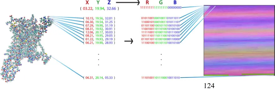
2.1. Transformation of MD trajectories into pixel representations readable by DNNs
113
To apply image-recognition (picture-recognition) technology in the analysis of the MD
114
trajectories for the various ligand-GPCR complexes, the complete MD trajectory for each complex
115
must be transformed into a pixel representation that constitutes the canonical input for these ML
116
algorithms. We developed a transformation that takes advantage of the similarities between the
117
components of proteins and picture representations: both are composed of bits of information, i.e.,
118
the pixels in a picture and the atom in a protein. The definition of pixels in terms of their values of
119
red, green, and blue (RGB) parallels the definition of the individual atoms by their coordinates X, Y,
120
and Z (XYZ). Consequently, a unique representation of the protein as a picture is obtained when each
121
atom of the protein is transformed into a pixel with an RGB value that corresponds to that atom’s
122
XYZ value (Figure 1).
123
124
Figure 1: Visual representation of a molecular structure. Each atom of the molecule (left) is identified by the set
125
of (x,y,z) coordinates as illustrated by the numerical set. The transformation to a 2D picture-like representation
126
is obtained by assignment to each pixel representing an atom (in sequential order from top left to bottom right)
127
by a pixel whose RGB value is the XYZ coordinate of the atom it represents (identified by the set of digital
128
values). This representation has the special property that each pixel (i.e. matrix element) always represents the
129
same atom in each frame from the trajectory of a particular protein.
130
Since this procedure is sensitive to the translational and rotational movements of the protein, the
131
trajectories are pre-processed by scrambling to remove bias from the original trajectory (see the next
132
section for details on the scrambling procedure).
133
2.2. Training and application of DNNs able to recognize ligand-dependent receptor conformations
135
2.2.1 General Protocol
136
The representation of a protein according to the rules described in section 2.1, above, encodes the
137
three-dimensional structure of a molecule into a two dimensional picture that can be fed directly into
138
an ML algorithm, such as the convolutional neural network utilized here, without any loss of
139
information (clearly, such a loss would occur if a conventional projection-like “picture” was taken of
140
the molecule). In the method of analysis presented here, this transformation is applied to each frame
141
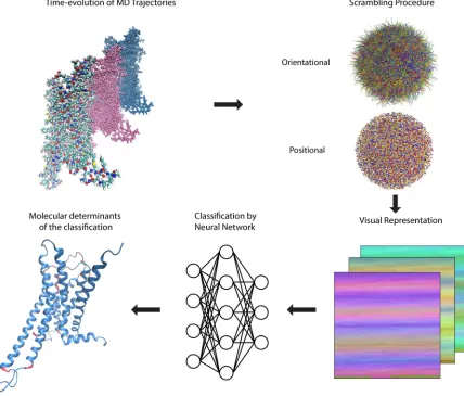
of the MD trajectory sequentially, and followed by the steps depicted in Figure 2.
142
143
Figure 2: Overview of the computer-aided inspection pipeline described in detail in the text. MD trajectories
144
representing the time evolution of each system are subjected to a scrambling procedure to erase positional and
145
orientational information and then each frame is converted into a visual representation suitable for feeding to a
146
deep convolution neural network for training, validation, and testing of classification accuracy. A sensitivity
147
analysis protocol is carried out to reveal the most important parts of the molecule (highlighted in red, see text
148
and subsequent figures for more details) used in the classification by the neural network, and collective variables
149
are extracted from the network to aid in further analysis.
150
The trajectories collected from MD simulations of ligand-GPCR complex of the serotonin
5-151
HT2AR and dopamine D2R (see Methods for details) were used to illustrate the application of the
152
pipeline described in Figure 2. The data submitted for the DNN contains the coordinates of the atoms
153
in the receptor structures sampled at the time-steps of the MD trajectories (frames), presented in the
154
form of the visual representation of these coordinates ( Figure 1), as well as the corresponding class
155
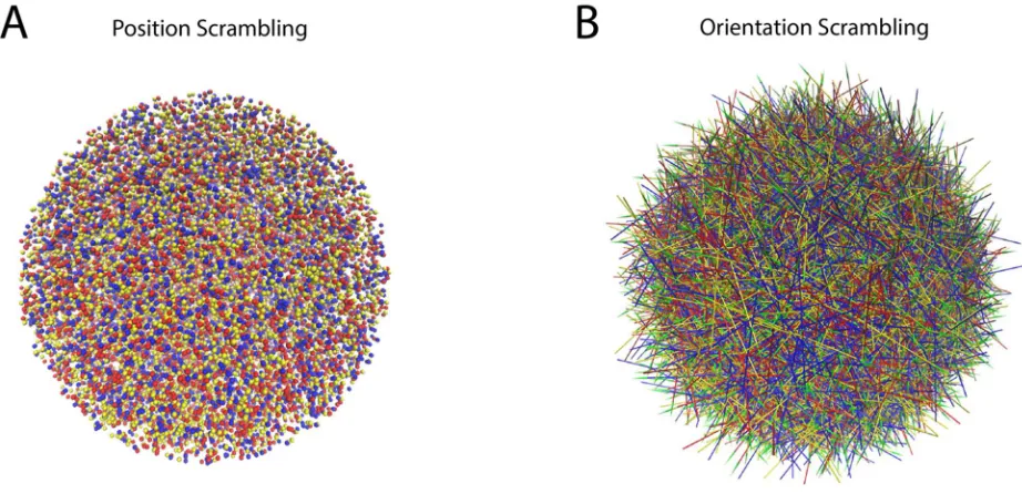
The scrambling protocol applied to the data prior to submission to the neural network (NN) is
157
an unbiasing step in which the position of each frame and its orientation are scrambled (randomly;
158
see Figure 3 for more information on the trajectory scrambling). This is undertaken in order to
159
eliminate from consideration by the NN of any differences among frames that originate not from the
160
time-dependent molecular dynamics, but from changes in position or orientation of the ligand-GPCR
161
complex. Thus, the scrambling directs the NN algorithm to consider only the intramolecular changes
162
of the protein induced by the ligands. This scrambling is introduced in our protocol to achieve the
163
same unbiasing that is attained in image classification tasks by random orientation of objects in
164
pictures (which forces the object recognition neural networks to understand the shapes and colors of
165
objects, independent of their background and orientation).
166
167
Figure 3: Illustration of the protocol for scrambling the frames of the MD trajectories. Each frame of each
168
trajectory was positionally scrambled by moving its center of mass to a randomly sampled coordinate within a
169
sphere of diameter 90 Å (the size of the largest dimension of the receptor). The orientation of the receptor was
170
scrambled by aligning a vector defined by two arbitrarily chosen atoms (preferably on an axis connecting the
171
intracellular and extracellular ends of the GPCR) to a random unit vector in spherical coordinates. (Note: for the
172
5-HT2AR, the two atoms chosen were atoms 3695 and 4346, which are the eta hydrogen (H η) of K6.32 and one
173
of the delta hydrogens (Hδ) of L7.34, respectively ) A. Illustrates the arbitrary positioning in space of the frames
174
belonging to different trajectories by showing the center of mass of the first 1000 frames of arbitrarily-chosen
175
trajectories from each class. Frames from a full agonist-bound trajectory are in blue, from partial agonist-bound
176
are yellow, from inverse agonist-bound are red B. Illustrates the arbitrary orientation of the frames from the
177
different trajectories: Green-tipped arrows with shafts going through atoms 3695 and 4346 are colored by the
178
same color scheme as in A, and drawn for each of the first 1000 frames of the same trajectories as in panel A.
179
The convolution neural network (Figure 2) was trained on training and validation sets, and
180
tested on the data set, following known ML protocols [15, 18] (see below, section 2.2.2). The results
181
for the 5-HT2AR (section 2.2.2) and D2R (section 2.2.3) systems were then analyzed as described below
182
in section 3 to identify the molecular determinants of the classification.
183
184
2.2.2 Pharmacological classification of the MD trajectories of 5-HT2AR-ligand complexes
185
The set of 5-HT2AR-bound pharmacologically distinct ligands chosen for this illustrative
186
application includes the full agonist serotonin (5-HT), the inverse agonist ketanserin (KET), and three
187
lysergic acid diethyl amide, LSD, and lisuride (LIS), and one is smaller, similar in size to 5-HT
(2,5-189
Dimethoxy-4-iodoamphetamine, DOI). The data set consists of 43,565 structures sampled with a 0.2
190
ns time-interval from the full and inverse agonist trajectories, and a 0.6 ns time-interval from the
191
partial agonist trajectories (to maintain a balance in the number of samples from each class). The
192
complete set of trajectory data, along with their corresponding class labels, was split into training,
193
validation, and test sets of size 24396, 10456, and 8713, respectively.
194
The 5-HT2AR complexes were subjected to the general protocol described in section 2.2.1 above.
195
The results for the 5-HT2AR test set quantify the accuracy of the neural network in predicting the class
196
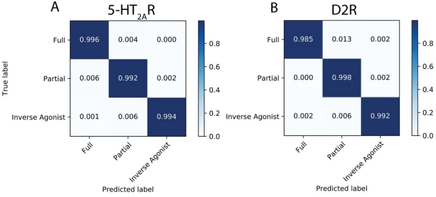
labels of pharmacological classifications of the 5-HT2AR ligands in the form of a confusion matrix
197
(Figure 4). The formulation of the confusion matrix relates the predicted class label of the test set
198
instances to their true class label. Each element of the confusion matrix is calculated as:
199
( , )= ∑ ,( , ) ;
ℎ
,( , ) = 1,0, ℎ= = (1)200
where ( , ) is the (row, column) index of the confusion matrix, is the number of instances in the
201
test set, is the true class label of instance , and is the class label of instance predicted by
202
the neural network. Each element is then normalized to the total number of instances in each class.
203
Results from the application of the analysis to the test set for the 5-HT2AR are presented in the
204
confusion matrix in both numerical and a color-coded visual form Figure 4A. The diagonal elements
205
represent the fraction of instances for which the neural network had correctly identified the class
206
label. Off-diagonal elements show the fraction of incorrectly labeled instances and identify the class
207
to which they were incorrectly attributed.
208
209
Figure 4: Results of the classification for the test set of the 5-HT2AR (A), and D2R (B). The coded coloring and
210
numbers show the proportion of times the neural network predicted correctly a class label (diagonal elements),
211
and the extent to which it failed to correctly predict the class label (off-diagonal elements) by confusing it with
212
another class.
213
In this illustration of the method for the 5-HT2AR, >99% of the frames in the test set were correctly
214
labeled (the diagonal of the confusion matrix in Figure 4A). This near-perfect accuracy achieved on
215
the test set suggests that the neural network is able to recognize and classify the ligand-dependent
216
receptor conformations presented by this data set, with most of the very few incorrectly labeled
217
instances (the off-diagonal elements) involving confusion of partial agonist labels. The molecular
218
2.2.3 Pharmacological classification of D2R-ligand trajectories
220
In order to test the generalizability of the method to MD trajectories of other GPCRs, we analyzed
221
trajectories of another class A GPCR, the D2R, bound to pharmacologically distinct ligands, namely
222
the full agonist (Dopamine, DA), inverse agonist (Sulpiride, SLP), and partial agonist (Aripiprazole,
223
ARI).
224
Following the same steps described above for the analysis of 5-HT2AR, the D2R trajectories (see
225
Methods) were subjected to the protocol described in section 2.2.1 above. The visual representations
226
of the coordinates from structures (frames) sampled every 0.4 ns from the trajectories of the
ligand-227
D2R complexes were randomly split into training, validation, and test sets of size 20017, 8580, and
228
7150, respectively. The accuracy of the neural network in predicting the class labels of the D2R ligands
229
in the test set is presented in Figure 4B as a confusion matrix (see Eq. 1 and section 2.2.2 for details
230
on how the confusion matrix was constructed). The same high accuracy achieved by the neural
231
network for the classification of the 5-HT2AR trajectories, is attained in the classification of the smaller
232
set of classes for the D2R system.
233
2.3 Identifying the molecular determinants of the classification
234
2.3.1 General Protocol
235
To reveal the identity of the molecular features that were most instrumental in the classification
236
decisions of the NN, we employ a sensitivity analysis approach in the category of visual saliency [19].
237
This sensitivity analysis is based on computing the gradient of the neural network’s classification
238
score for a particular label (i.e., how likely the network believes a picture to be in each class), with
239
respect to each of the pixels of the input image. The higher the gradient for a particular pixel, the
240
more attention the neural network paid to it in making the classification.
241
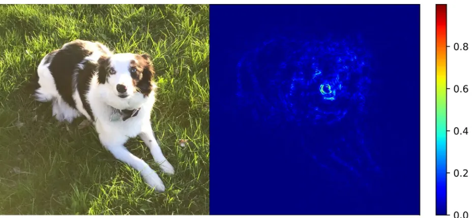
Figure 5 shows an example of this type of sensitivity analysis applied to a traditional image
242
classification. Here a deep neural network has correctly labeled a picture as “dog”, and the part of
243
the picture that the DNN utilized to make the classification is highlighted in the heat map (also called
244
“attention map”) next to it that color-codes the magnitude of the gradient for each pixel. Clearly, the
245
attention map in Figure 5 highlights (in the collection of highest gradient values) the pixels that
246
correspond to the dog, designating them as those having been the most important pixels for
247
classifying the picture correctly.
248
249
Figure 5: Sensitivity analysis applied to an image of a dog. For the heat map (attention map) on the right the
251
color bar quantifies the gradient of each pixel with respect to how likely the neural network considers this image
252
to be of a dog. This highlights the pixels that the neural network considered to be the most important for the
253
classification of the picture. The pixels that correspond to the outline of the dog are seen to be the most important
254
for the classification and thus have the highest gradient.
255
256
2.3.1 Application to the sensitivity analysis to the 5-HT2AR classifications
257
We applied this sensitivity analysis approach to identify the features used by the NN to classify
258
correctly the test frames as those corresponding to the 5-HT2AR bound to a full agonist. Figure 6A
259
shows an attention map calculated from the ligand-bound 5-HT2AR test set. This attention map was
260
obtained by averaging the attention maps of 1000 instances (trajectory frames) of the full agonist
261
bound 5-HT2AR. In this panel, the protein is represented by a 71x71 pixel matrix containing the atoms
262
of the receptor protein (20 atoms are missing from the C terminus) and constructed as described in
263
Figure 1. The elements are colored according to the color scheme with the largest gradient value
264
representing the highest importance of the atom in the classification task. The calculation of the
265
average takes advantage of the property of the visual representation of the protein in which each
266
pixel always represents the same atom.
267
To be able to relate the contributions of the identified key atoms and groups in the context of
268
structural regions of the protein, we show in Figure 6B the same data as in the attention map (panel
269
6A), but in a different representation in which all the pixels (i.e., atoms) are listed on the X axis
270
sequentially, labeled with their generic numbering that identifies the TM segments of the GPCR
271
protein. Applying to Figure 6B an importance cutoff value of 0.15 (chosen by inspection of the
272
attention map), the residues considered to be most important in the classification of the ligand bound
273
to the receptor are found to reside in the middle and the extracellular ends of TMs 2-5 (positions 2.56,
274
2.65, 3.28, 4.58, 4.59, 4.62, 4.63, 4.67, and 5.35-5.37, residues labeled with the generic
Ballesteros-275
Weinstein numbering[20]), at the intracellular ends of TMs 2 and 3 (positions 2.38 and 3.55) and in the
276
extracellular loops ECL1 and ECL2, as well as intracellular loops ICL2 and ICL3 (the pieces of which
277
that were identified as important exchange between loop and helical extensions of TM5 and TM6
278
throughout the trajectories). There is a roughly even distribution between important residues that
279
reside in the loops and the helices. These sites are indicated on the 5-HT2AR structure in Figure 6C.
280
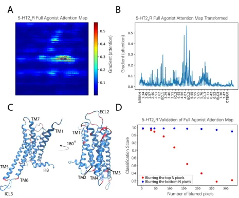
282
Figure 6: Identification of the molecular determinants of the classification of the full agonist bound to the
5-283
HT2AR. A: The full agonist attention map shown was obtained as the average of 1000 attention maps calculated
284
from 1000 instances of the full agonist bound to the 5-HT2AR. B: Representation of the (average) attention map
285
in panel A in which all the pixels (i.e., atoms) are listed on the X axis. The tick marks on the X axis identify
286
residues labeled with the generic Ballesteros-Weinstein numbering[20]. The gradient values calculated for the
287
classifier for individual atoms is on the Y axis; it indicate the order of importance (salience) of each atom for the
288
classification. C: The positions of the most important residues for the classification are indicated (in orange) on
289
the ribbon representation (in blue) of the 5-HT2AR model structure. The highlighted residues contain atoms
290
whose gradient (attention) is >0.15. D: Validation of the attention map by evaluation of the effect of blurring
291
increasing numbers of pixels (atoms) in the representation of the protein complex. Orange dots indicate the
292
results of blurring increasing numbers of pixels identified to have the lowest gradient (least important). Blue
293
dots indicate the results of blurring pixels with the highest gradient (most important). The number of atoms
294
blurred is shown on the X axis; the Y axis shows the corresponding classification score of full agonist for the
295
blurred images.
296
To verify further the role of these specific structural motifs in the classification produced by the
297
neural network, we compared the effect of blurring the pixels with the highest gradient (most
298
important; salient) to those with the lowest gradient (unimportant). In this procedure, sets of pixels
299
corresponding to a number N of least-important atoms for all classes, were blurred in the test set by
300
replacing them with Gaussian noise. This erased the information that these pixels confer to the neural
301
network. The classification score computed for such an altered image represents the probability of an
302
image belonging to a particular class, and the sum over all classes is unity. The same blurring
303
procedure was then repeated for the same number of pixels with the highest gradient (importance)
304
The results of this analysis for the full agonist-bound class (in Figure 6D), show that when the
306
most important pixels are blurred (blue dots), the classification score quickly decreases to the chance
307
rate (~0.33 for 3 classes) with 250 blurred pixels. This means that the network is no longer able to
308
identify this instance as bound to full agonist. However, after blurring the same and even larger
309
numbers of unimportant pixels (orange dots), the neural network is still able to identify the instance
310
as belonging to the full agonist bound class (with a classification score >0.9).
311
2.3.2 Sensitivity analysis applied to the classification of the D2R complexes
312
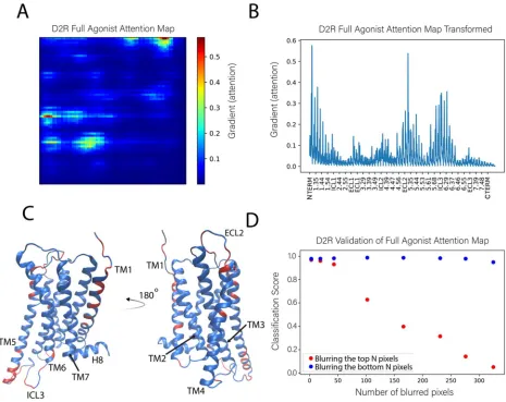
313
Figure 7: Identification of the molecular determinants of the classification of the full agonist
314
bound to the D2R. A: The full agonist attention map shown was obtained as the average of 1000
315
attention maps calculated from 1000 instances of the full agonist bound to the D2R. B: Representation
316
of the (average) attention map in panel A represented as in figure 6B. C: The positions of the most
317
important residues for the classification are indicated (in orange) on the ribbon representation (in
318
blue) of the D2R model structure. The highlighted residues contain atoms whose gradient (attention)
319
is >0.15. D: Validation of the attention map following the same procedure as described in figure 6D.
320
The results of applying the sensitivity analysis to the pharmacological classification of
ligand-321
bound complexes of the other class-A GPCR, D2R, shown in Figure 4B, are summarized in Figure 7.
322
Using the same importance cutoff value of 0.15 as in the analysis of the 5-HT2AR, we find that the
323
most important residues in the classification of the ligand-D2R complexes reside in the middle and
324
the extracellular ends of TMs 1, 4, and 5 (positions 1.29, 1.30, 1.33, 1.34, 1.37, 1.38, 1.42, 1.46, 1.51, 4.53,
325
4.62, 5.35, 5.36, 5.39, 5.40, and 5.44), at the intracellular ends of TMs 5-6 (positions 5.64, 5.69, 5.70,
5.72-326
5.74, 6.29, and 6.33) and in the extracellular loop ECL2, as well as intracellular loops ICL2 and ICL3.
327
the most important residues found by the attention map analyses of the D2R and 5-HT2AR
329
trajectories. Among the most important regions found by both analyses was the intracellular ends of
330
TM5 and TM6, the extracellular end of TM4 and TM5, as well as ECL2, ICL2, and ICL3. Remarkably,
331
among the most important residues of both analyses was residues 4.62 and 5.36 on the extracellular
332
ends of TM4 and TM5, respectively. Multiple analogous residues of the ECL2 as well were identified
333
in both analyses, including the highly conserved cysteine (C227 in 5-HT2AR and C182 in D2R) that
334
makes a disulfide bond with C3.25 and was shown to be critically important to the function of many
335
class A GPCRs[21].
336
2.4 Dynamic differences discriminated by the DNN in the regions most important
337
for the classification decisions of ligand-bound GPCRs
338
To gain additional insight into the nature of dynamic differences discriminated by the DNN in
339
the regions most important for the classification decisions, we compared the conformational
340
dynamics of specific residues identified by the atoms with high importance for the classification.
341
2.4.1 5-HT2AR complexes
342
Starting with the most important region identified in Figure 6B, i.e., the second extracellular loop
343
(ECL2), we evaluated the dynamic range of the top hit of the sensitivity analysis for the 5-HT2AR
344
bound to the full agonist, compared to the aligned trajectories of the 5-HT2AR complex with a full
345
agonist and the inverse agonist. Figure 8A shows the sampling of the epsilon carbon (Cε) atom of F222
346
in ECL2. Although the starting structures of the GPCR in all 5-HT2AR-ligand bound complexes were
347
highly similar (see Methods for details on docking), the conformational space sampled by this region
348
diverged over the course of the simulations. As Figure 8A shows, ECL2 of the 5-HT2AR bound to
349
the inverse agonist (KET) samples two distinct states over the trajectories in the dataset (red and
350
orange points in Figure 7A), with the red points indicating conformations in which F222 is almost
351
exclusively pointing inward, towards the binding pocket and TMs 6 and 7 (see Figure 8B bottom left).
352
In the other trajectory (orange points) of the KET-bound 5-HT2AR, a section of the ECL2 including
353
F222 prefers an alpha-helical conformation, resulting in F222 pointing mostly away from the binding
354
pocket towards the extracellular side (Figure 8B top left), with some brief overlap with the sampling
355
of the red trajectory. Notably, both of these conformations are distinct from those sampled by the
5-356
HT2AR bound to the full agonist 5-HT (blue and purple points in Figure 8A). In the 5-HT-bound
357
trajectories, the section of the ECL2 containing F222 samples disordered/unfolded conformations in
358
which F222 primarily occupies a region of space away from the binding pocket than the KET-bound
359
(orange) trajectory, but shifted closer to TMs 1 and 2. Interestingly, in the trajectories of the 5-HT2AR
360
bound to partial agonists, the Cε of F222 samples regions of space that overlap with both of the
361
regions sampled in the trajectories of the 5-HT2AR bound to full and inverse agonist.
362
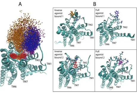
363
365
Figure 8. Conformational dynamics of residue F222 in ECL2 identified by the positions of the epsilon carbon
366
atom Cε of F222 in the simulation trajectories. A. Sampling of the coordinates of Cε of F222 (atom 2532), the
367
top hit of the sensitivity analysis for serotonin (5-HT), in the aligned trajectories of the 5-HT2AR bound to the
368
inverse agonist ketanserin (KET) (red and orange) and the full agonist 5-HT (blue and purple). B. Representative
369
frames from each of the four trajectories shown in the previous panel. F222 is colored solidly according to the
370
bound ligand, ketanserin (red and orange) and serotonin (blue and purple)
371
372
On the intracellular side of the receptor, we followed the conformational dynamics of residue
373
R310 in ICL3, containing the epsilon hydrogen (Hε) identified as a highly salient atom. Figure 9A
374
shows the sampling of the Hε in the aligned trajectories of the 5-HT2AR bound to full 5-HT (in blue)
375
and KET (in red). The two representative frames from the trajectories, shown in Figure 9B, illustrate
376
the conformation of the ICL3 sampled by each class. There is near perfect separation between the
377
space sampled by the Hε atom of R310 over the full and inverse agonist bound trajectories,
378
confirming that this residue, identified as important by the neural network, indeed confers a large
379
amount of information about whether and how the ensembles of ligand-dependent conformations
380
differ.
381
382
384
Figure 9. Conformational dynamics of residue R310 in ICL3 identified by the epsilon hydrogen highlighted by
385
the sensitivity analysis. A. Sampling of the coordinate of the epsilon hydrogen of R310 (atom 3535) in the ICL3,
386
over all of the aligned trajectories of the 5-HT2AR bound to the inverse agonist ketanserin (red) and the full
387
agonist serotonin (blue). B. Example frames from each class of trajectories shown in panel A. R310 is colored
388
solidly according to the bound ligand, KET (red) and 5-HT (blue)
389
The conformations of the partial agonist trajectories are differentiated by a different set of
390
residues. The ICL3 of the partial agonist is not differentiated by the R310 Hε, as in the partial
agonist-391
GPCR complex this atom samples both of the spaces shown in Figure 9A, with some preference for
392
the trajectory of the full agonist. Instead, Figure 10 shows that the conformation of the ICL3 in the
393
partial agonist trajectories is different from the other complexes in that it preserves throughout the
394
helical structure of the residue segment 306 to 310 of TM6, whereas the same piece of ICL3 samples
395
a disordered/unfolded conformation in both the full and inverse agonist-bound trajectories (shown
396
in Figure 9). This is evidenced by the sampling of T307 in the ICL3, a residue identified as important
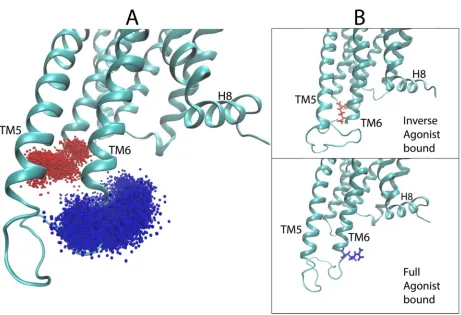
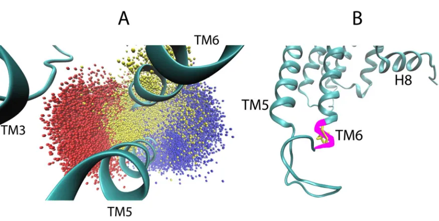
397
399
Figure 10. Conformation of the ICL3 of the 5-HT2AR in complexes with full- partial- and inverse-agonists. In
400
most of the partial agonist trajectories, a piece of the ICL3 (magenta) forms an extra helical turn of TM6. In the
401
full and inverse agonist-bound trajectories, this piece of the ICL3 is disordered/unfolded, with T307 pointing
402
inwards towards TM3 in the inverse agonist trajectories, and pointing away from TM3 in the full agonist bound
403
trajectories. A. The sampling of the coordinate of the gamma oxygen of T307, an atom identified as important in
404
the attention map of the partial agonist, for all the trajectories of the 5-HT2AR bound to full agonist (in blue),
405
inverse agonist (red), and partial agonist (yellow). B. Illustrative frame from partial agonist bound trajectories
406
showing the extended helical conformation of the ICL3. T307 is colored in yellow and the extra helical turn is
407
colored in magenta.
408
2.4.2 D2R complexes
409
For the dopamine receptor complexes we again focused first on ECL2 which was identified as
410
important for the classification of the ligand-D2R complexes. Figure 11A shows the time dependence
411
in the trajectory of the values taken by the dihedral angle across the disulfide bond formed between
412
C182 in the loop and C3.25 (in TM3) over the full-agonist (DA) bound and inverse agonist (SLP)
413
bound trajectories of the D2R. For the majority of the SLP-bound trajectories, the ECL2 samples
414
conformations that are never sampled in the DA-bound trajectories. This is evidenced in the figure
415
by the difference in the dihedral angle of the disulfide bond between the two cysteines. The DA
416
trajectories (blue) remain in an angle range around -100, never sampling above -40, whereas the
417
SLP (red) trajectory samples mostly around 100. A simple cutoff of 0, for example, can distinguish
418
a majority of the inverse agonist frames. These differences in angle values determine different 3D
419
orientations of the ECL2 which thus becomes a salient feature for describing the differences in the
420
ensemble of conformations sampled by the trajectories of D2R bound to the full and inverse agonist.
421
423
Figure 11: Involvement of residue C182 identified by the D2R sensitivity analysis in the discrimination of
424
ECL2 structures. A: The dihedral angle is measured along the disulfide bond between C182 and C3.25 for the
425
full agonist bound (blue) and inverse agonist bound (red) trajectories. B: Illustrative frames from the trajectories
426
in panel A representing the two dihedral angle states. The ligand for each class (Dopamine for full agonist, and
427
Sulpiride for the inverse agonist ) is shown in function colored CPK.
428
Like in the 5-HT2AR complexes, the residues in the extensions of TM5 and TM6 are important for
429
the classification by the DNN. For the dynamic context, we compared residues K5.70 and T5.74 ( both
430
identified as important by the D2R sensitivity analysis) of the extension of TM5 in the aligned
431
trajectories of the ligand-D2R complexes. Interestingly, inspection of the trajectories shows a
432
difference in the preference of helical conformation of the intracellular end of TM5 dependent on the
433
backbone hydrogen bond between these residues. The full-agonist bound trajectories preferred the
434
helical conformation while the inverse-agonist bound trajectories preferred a disordered
435
conformation. Figure 12A shows a measure of the helicity involving residues K5.70-T5.74 in the
436
trajectories, quantified by the distance between the backbone oxygen of K5.70 and the backbone
437
amide hydrogen of T5.74. The majority of frames in the DA-bound trajectories exhibit a smaller
438
distance than those of the SLP-bound trajectories, because K5.70 and T5.74 form part of a helical
439
structure for most of the full agonist trajectory, whereas in the inverse agonist bound trajectories these
440
residues are in a more disordered conformation. Figure 12B presents example frames from the
441
ensemble of conformations sampled by D2R bound to the full and inverse agonist, underscoring the
442
clear difference in helicity of the TM5 region and thus the structural context of the identified
443
importance of the two residues in the classification by the DNN.
444
446
Figure 12: Residues K5.70 and T7.54 identified by the D2R sensitivity analysis determine the helicity of the
447
intracellular TM5 extension. A: The distance between the backbone oxygen of K5.70 and the backbone amide
448
hydrogen of T5.74 along trajectories of D2R bound to the full agonist (in blue) and the inverse agonist (red).
449
B: Illustrative frames from the trajectories in panel A chosen for the distinct difference in the distance, and its
450
effect on the helicity of the intracellular end of TM5.
451
452
3. Discussion
453
The machine learning-based approach we developed and illustrated here with applications to
454
the classification of ligand-determined GPCR conformational properties, points to some new
455
directions taken by methods for MD trajectory analysis. In particular, analyses involving machine
456
learning are growing in popularity as a greater variety of scientific questions is being addressed with
457
MD simulations, and the systems targeted are increasingly complex. The data generated by these
458
ever larger scales of simulation, accrued for large systems that require longer simulation times, is
459
moving the field into the realm of Big Data Science [22]. A recent review of fundamental MD
460
problems that could be addressed in the framework of Machine Learning (ML) [23], shows how ML
461
has the potential to tackle problems arising from large scale simulations, and that it has already had
462
profound impact on alleviating them (see Noe et al.[23] and references therein).
463
The work we present supports the overall optimistic outlook regarding the potential of ML
464
algorithms to extract important functional information from MD simulation trajectories in the usual
465
structural and dynamic context of molecular mechanisms. An imperative in this respect, is the
466
development of approaches to translate the results obtained with DNN-based protocols into clear
467
structural information in order to illuminate the underlying mechanisms in a physics-based context.
468
By extracting automatically the functional information we achieved a major reduction in
469
dimensionality of MD Big Data into a collection of salient structural motifs that efficiently describe
470
the differences between ensembles of conformations sampled by each tested state. The results of this
471
study are particularly encouraging, despite the limited scope of the test framework used in the
472
illustration, as the approaches (i)-classify correctly the ligand-bound GPCRs, (ii)-identify the
473
molecular determinants of the classification, and thus also the dynamic differences in the regions
474
most important for the classification decisions.
475
Only 5 ligands for the serotonin 5-HT2AR and 3 for the dopamine D2 receptors were used in this
476
limited test, but the results show that through the methodology described herein, a DNN is able to
477
identify the relation between the functional properties of ligand-receptor complexes and the
478
ensemble of conformations that they sample within MD trajectories. Due to the limited sampling of
479
both configurational space and the classification field, the trajectory data served here only to
480
exemplify the ability of the method to distinguish functional states of a GPCR, not to reach any
481
conclusion about the significance of the functional states themselves. And yet, it is encouraging to
482
differences are common to both the 5-HT2AR and D2R, and are regions known to be important for
484
GPCR activation. Thus, the ECL2 has been shown to play a critical role in class A GPCR activation[24],
485
taking on ligand-dependent conformations that are important for function[24-27]. The regions of the
486
intracellular side of the receptor identified by our analysis, including the two ends of the ICL3 (i.e.,
487
the N-terminus of the loop which continues TM5, and its C-terminus which elongates the start of
488
TM6), are also critically important for GPCR activation as these sites directly interact with the G
489
protein[28] . As such, they are involved in the opening, observed in active GPCRs[29], of the
490
intracellular side of the receptor.
491
It is noteworthy, however, that while they serve to discriminate between ligand classes, the
492
dynamics of these salient motifs differ between the 5-HT2AR and D2R systems. This is further
493
reassuring because even if their role in recognizing the G protein, say (for the ICL3 motifs) is the same,
494
they must respond to different G proteins in different functional contexts. However, that the
495
structural motifs mentioned above were similarly sensitive to the bound ligand in both systems is
496
concordant with the evidence that class A GPCRs involve similar structural motifs in the
497
pharmacological response. Collectively, the accuracy and agreement between the sensitivity analyses
498
applied to the 5-HT2AR and D2R trajectories suggests that this method should generalize to other
499
GPCR simulation studies, including trajectories of other ligand-GPCR complexes in diverse coupling
500
pathways.
501
The characteristics of the novel method of analysis described here support its applicability not
502
just to classifications of receptor activity (efficacy), but by finding ligand-dependent differences in
503
MD trajectories of GPCRs, it is especially promising for the classification of ligand bias in functional
504
selectivity as well. Our ongoing work is exploring this application, as well other functional
505
classifications being studied such as membrane lipid composition or the presence or absence of an
506
action such as ion release.
507
4. Materials and Methods
508
Building homology model of the GPCRs
509
MODELLER (v.9.18)[30] was used to generate the sets of homology models of the human
5-510
HT2AR, and the human dopamine D2R. Briefly, Modeller generates 3D homology models of
511
proteins using sequence alignments between the target and homologous proteins, as well as
512
experimental structural data (e.g. x-ray or cryoEM structures from homologous proteins). These
513
models are generated by optimally satisfying spatial restraints that are derived from the template
514
structure(s). Because template-derived spatial constraints inform model construction, there is
515
tension between choosing the most homologous template structures and providing Modeller with a
516
set of template structures that possess enough sequential/structural heterogeneity so that the
517
resultant set of homology models are significantly structurally diverse.
518
Modeling the 5-HT2AR: Three sets of sequence alignments/crystal structures were used as templates
519
in Modeller:
520
- Set 1 consisted of two structures of the human 5HT2BR (PDBID: 4ib4 and 5tvn);
521
- Set 2: included two structures of the human 5HT2BR (PDBID: 4ib4 and 5tvn) and
522
two structures of the human 5HT1BR (PDBID: 4iaq and 4iar);
523
- Set 3: included all the structures in Set 2, augmented by 2 structures of the human
ß2-524
adrenergic receptor b2AR (PDBID: 4lde and 4ldl).
525
Each of these template structures includes the receptor bound to one of its agonists. For each
526
template set, Modeller was used to generate 1,000 homology models of the 5-HT2AR.To select a
527
ability to discriminate between 5-HT2AR agonists and decoy ligands (i.e. ligands that are predicted
529
to not bind 5-HT2AR); this characterization was performed by employing a multistep procedure.
530
First, a set of 47 known human 5-HT2AR agonists was obtained from the IUPHAR/BPS database
531
[accessed on May 1st, 2017] [31]. These agonists were then submitted to the DUD-E server [accessed
532
on May 5th, 2017] [32], which generated a set of 3,229 decoy structures. Briefly, DUD-E generates
533
decoy structures that have similar physical chemistry properties (e.g. molecular weight, hydrogen
534
bond donors/acceptors, rotatable bonds, etc.) but have a dissimilar topology. Schrodinger’s LigPrep
535
software (v. 40015) was used to convert the agonist set and DUD-E SMILES descriptions into 3D
536
ligand models.
537
Next, the 3 sets of 1,000 Modeller homology models were prepared for docking studies using
538
Schrodinger’s Protein Preparation Wizard (v. 2016-2) [33]; this procedure added hydrogen atoms
539
and created the disulfide bond between C3.25(148) and ECL2 loop residue C227. Schrodinger’s
540
Glide software (v.34014) [34] was used to dock each of the 47 agonist and 3,229 decoy structures
541
into the models in the 3 sets (3,000 models total), using standard precision; for each receptor/ligand
542
complex, Glide calculates a ‘GlideScore’, which is an approximation of the ligand’s free energy of
543
binding to the protein.
544
Each model’s ability to discriminate between true agonist and decoy structures was quantified
545
using the set of ligand GlideScores. The set that only used 5HT2B as input templates was the most
546
discriminating model overall and was used for subsequent docking studies, described below.
547
Molecular construct for D2R
548
The crystal structure of the D2 dopamine receptor bound to Risperidone [27] was used as
549
starting construct. The missing intracellular loop IL2 was modelled using MODELLER [30]. The
550
long intracellular loop IL3, substituted by T4 lysozyme in the crystal construct, was replaced by a
551
10mer of Gly residues, inserted between S229 and Q365.
552
Parametrization and docking of the molecular models
553
MOL2 files for the 5-HT2AR ligands (5-HT, Ketanserin, LSD, Lisuride, and DOI) as well as for
554
the D2R ligands (Dopamine, Sulpiride, Aripiprazole) were obtained from the ZINC [35] database.
555
The amide nitrogen in these compounds was protonated and docking poses were generated into
556
the identical 5-HT2AR homology model and into the D2R structure using the Induced Fit [36-38]
557
protocol in the Schrodinger Suite. A starting binding pose was chosen for each ligand based on the
558
e-modal score and comparison to experimental data [25-27, 39-43]. Parameters for the CHARMM36
559
[44] force field each ligand were obtained by analogy from the CGenFF program [45, 46].
560
Parameters with analogy penalties greater than or equal to 5 were optimized using the Force Field
561
Toolkit (ffTK) [47]. Quantum mechanical calculations were made at the Hartree-Fock level of theory
562
using the Gaussian software [48].
563
Molecular dynamics simulations
564
The GPCR systems were simulated in atomistically explicit membrane environments following
565
established lab protocols (e.g., see REFs). For the simulation of 5-HT2AR-ligand complexes the
566
molecular model was inserted into a membrane containing 144:16 POPC:Cholesterol molecules of
567
in each leaflet. The membranes were built using the CHARMM-GUI[49] and equilibrated using the
568
NAMD[50] software ver2.12 according to an equilibration protocol generated[51] by the
569
CHARMM-GUI. After inserting the protein into the equilibrated membrane, the protein-membrane
570
complex was surrounded by a 0.15 M NaCl solution with a hydration number of 80 water
571
structures were embedded, using the CHARMM-GUI, into a membrane consisting of 180:18
573
POPC:Cholesterol molecules per leaflet, and was solvated and ionized using the same conditions as
574
above.
575
Each complete system was equilibrated under the NPT ensemble (T=310K) in NAMD
576
according to a previously established multistep equilibration protocol [16, 52] before running
577
approximately 1.5 microsecond long trajectories for each under the NVT ensemble (T=310K). The
578
production runs were carried out with the ACEMD3 [53] software with a 4 femtosecond time-step
579
and with all the standard simulation parameters [5, 9, 16, 52] following established and
580
documented protocols (REFs as indicated).
581
Machine Learning procedures
582
Building the DNN: A custom Densely Connected Neural Network [15, 18] was constructed, with 4
583
dense blocks containing 6, 12, 36, and 24 layers, respectively, a growth rate of 48 filters per layer, 96
584
initial filters, and a reduction ratio of 0.5, in Keras [54] with a Tensorflow [55] backend based on an
585
established implementation [56]
586
Classification of the trajectories: Each frame of the scrambled trajectories was converted into a visual
587
representation using the previously-described algorithm. Each frame was assigned a label
588
according to its functional class (0 for full agonist bound, 1 for partial agonist bound, and 2 for
589
inverse agonist bound). The frames were randomly split into a training, validation, and test set in
590
the ratio of 56:24:20, respectively. The neural network was trained on the training and validation
591
sets, and tested on the test set. The reported score is based on the test set.
592
Sensitivity analysis (keras-vis): The sensitivity analysis was performed by computing the gradient
593
using the visual saliency package provided by keras-vis [57] with guided back-propagation.
594
595
Author Contributions: Conceptualization: A.P. and H.W. ; methodology: A.P.; formal analysis:
596
A.P., molecular modeling: D.M.S. and G.M.; molecular dynamics simulations: A.P., D.M.S., G.M.,
597
and G.K.; writing—original draft preparation: A.P. and H.W.; writing— all authors interpreted the
598
data and participated in manuscript writing and editing; visualization: A.P. and G.M.; supervision:
599
H.W.; funding acquisition: H.W. and G.K.
600
Acknowledgement: The work was supported by the 1923 Fund and Cofrin Center for Biological
601
Information (to H.W. and G.K.), NSF grant BIGDATA: IA: Collaborative Research: In Situ Data
602
Analytics for Next Generation Molecular Dynamics Workflows (NSF #1740990) and NIH grant
603
EY028314 (to G.K. ). MD simulations used resources of the Oak Ridge Leadership Computing
604
Facility (INCITE allocation BIP109), which is supported by the Office of Science of the U.S.
605
Department of Energy under Contract No. DE-AC05-00OR22725, and an allocation at the National
606
Energy Research Scientific Computing Center (NERSC, repository m1710) supported by the Office
607
of Science of the U.S. Department of Energy under Contract No. DE-AC02-05CH11231. Local
608
computational resources of the David A. Cofrin Center for Biomedical Information in the HRH
609
Prince Alwaleed Bin Talal Bin Abdulaziz Alsaud Institute for Computational Biomedicine at Weill
610
Cornell Medical College are gratefully acknowledged.
611
612
Conflicts of Interest: The authors declare no conflict of interest.
613
References
615
1. Smith JS, Lefkowitz RJ, Rajagopal S. Biased signalling: from simple switches to allosteric microprocessors.
616
Nat Rev Drug Discov. 2018;17(4):243-60.
617
2. Berg KA, Maayani S, Goldfarb J, Scaramellini C, Leff P, Clarke WP. Effector pathway-dependent relative
618
efficacy at serotonin type 2A and 2C receptors: evidence for agonist-directed trafficking of receptor stimulus.
619
Mol Pharmacol. 1998;54(1):94-104.
620
3. Urban JD, Clarke WP, von Zastrow M, Nichols DE, Kobilka B, Weinstein H, et al. Functional selectivity and
621
classical concepts of quantitative pharmacology. J Pharmacol Exp Ther. 2007;320(1):1-13.
622
4. Weinstein H. Hallucinogen actions on 5-HT receptors reveal distinct mechanisms of activation and
623
signaling by G protein-coupled receptors. Aaps Journal. 2005;7(4):E871-E84.
624
5. Shan JF, Khelashvili G, Mondal S, Mehler EL, Weinstein H. Ligand-Dependent Conformations and
625
Dynamics of the Serotonin 5-HT2A Receptor Determine Its Activation and Membrane-Driven Oligomerization
626
Properties. Plos Computational Biology. 2012;8(4).
627
6. Wingler LM, Elgeti M, Hilger D, Latorraca NR, Lerch MT, Staus DP, et al. Angiotensin Analogs with
628
Divergent Bias Stabilize Distinct Receptor Conformations. Cell. 2019;176(3):468-+.
629
7. Perez-Aguilar JM, Shan JF, LeVine MV, Khelashvili G, Weinstein H. A Functional Selectivity Mechanism
630
at the Serotonin-2A GPCR Involves Ligand-Dependent Conformations of Intracellular Loop 2. Journal of the
631
American Chemical Society. 2014;136(45):16044-54.
632
8. Hollingsworth SA, Dror RO. Molecular Dynamics Simulation for All. Neuron. 2018;99(6):1129-43.
633
9. Razavi AM, Khelashvili G, Weinstein H. A Markov State-based Quantitative Kinetic Model of Sodium
634
Release from the Dopamine Transporter. Sci Rep. 2017;7:40076.
635
10. Song X, Jensen MO, Jogini V, Stein RA, Lee CH, McHaourab HS, et al. Mechanism of NMDA receptor
636
channel block by MK-801 and memantine. Nature. 2018;556(7702):515-9.
637
11. Shaw DE, Dror RO, Salmon JK, Grossman JP, Mackenzie KM, Bank JA, et al. Millisecond-Scale Molecular
638
Dynamics Simulations on Anton. Proceedings of the Conference on High Performance Computing Networking,
639
Storage and Analysis. 2009.
640
12. Motlagh HN, Wrabl JO, Li J, Hilser VJ. The ensemble nature of allostery. Nature. 2014;508(7496):331-9.
641
13. Chen M, Mao SW, Liu YH. Big Data: A Survey. Mobile Netw Appl. 2014;19(2):171-209.
642
14. Frankel F, Reid R. Big data: Distilling meaning from data. Nature. 2008;455(7209):30-.
643
15. Huang G, Liu Z, van der Maaten L, Weinberger KQ. Densely Connected Convolutional Networks. Proc
644
Cvpr Ieee. 2017:2261-9.
645
16. Khelashvili G, Stanley N, Sahai MA, Medina J, LeVine MV, Shi L, et al. Spontaneous inward opening of the
646
dopamine transporter is triggered by PIP2-regulated dynamics of the N-terminus. ACS Chem Neurosci.
647
2015;6(11):1825-37.
648
17. LeVine MV, Weinstein H. NbIT - A New Information Theory-Based Analysis of Allosteric Mechanisms
649
Reveals Residues that Underlie Function in the Leucine Transporter LeuT. Plos Computational Biology.
650
2014;10(5).
651
18. Pleiss G, Chen D, Huang G, Li T, van der Maaten L, Weinberger KQ. Memory-efficient implementation of
652
densenets. arXiv preprint arXiv:170706990. 2017.
653
19. Karen Simonyan AV, Andrew Zisserman. Deep Inside Convolutional Networks: Visualising Image