DOI: 10.1051/epjconf/201610603008 C
Owned by the authors, published by EDP Sciences, 2016
Application of the Subgroup Decomposition Method (SDM)
for Reactor Simulation
Nathan Roskoff, William Walters, and Alireza Haghighat
Nuclear Engineering Program, Mechanical Engineering Department, Virginia Tech, Arlington, VA, USA
Abstract.The performance of the TITAN-SDM algorithm for solving a reactor pressure vessel dosimetry problem is evaluated. Douglass and Rahnema recently developed the he subgroup decomposition method (SDM); a methodology which directly couples a consistent coarse-group transport calculation with a set of “decomposition sweeps” to provide a fine-group flux spectrum. The SDM has been implemented into the TITAN three-dimensional transport code and has been shown to accurately solve core criticality problems while significantly reducing computation time. This paper addresses the use of SDM for fixed-source problems. The VENUS-2 dosimetry benchmark problem is selected with an emphasis on fast neutron analysis; therefore, material cross sections are generated from the BUGLE-96 library considering neutron energies greater than 0.1 MeV. The accuracy and efficiency of TITAN-SDM is evaluated by comparison with a standard TITAN multigroup calculation.
1. Introduction
Recently, Douglass and Rhanema developed a novel method for performing multigroup transport calculations for core physics application, i.e. core criticality calculation. This method, referred to as Subgroup Decomposition Method (SDM) [1], is an extension of the standard cross-section condensation process [2] that preserves spectral accuracy as well as the energy-angle coupling which is generally lost in standard condensed-group transport calculations. The SDM can effectively generate a detailed fine-group flux spectrum from a coarse-fine-group transport calculation.
The SDM algorithm is implemented into the TITAN three-dimensional SN transport code [3], referred to as TITAN-SDM. TITAN-SDM has been previously demonstrated for core criticality calculations on both a one- and two-dimensional Very High Temperature Reactor (VHTR) core model [4]. The results demonstrated that, for a core criticality problem, the SDM algorithm is capable of significantly reducing computation time while maintaining adequate accuracy in both the eigenvalue and flux distribution.
In this paper, the performance of TITAN-SDM for a fixed-source reactor dosimetry problem is evaluated based on a model of the VENUS-2 benchmark problem [5]. Material cross-section information is generated from the BUGLE-96 library [6] which includes 47-group neutron and 20-group gamma data derived from ENDF/B-VI. The analysis considers fast neutron dosimetry; neutrons with energy of
0.1 MeV or greater are of concern, therefore a 26-group cross-section library is used. Reaction rates of 4 different dosimeters (58Ni(n,p),103Rh(n,n),237Np(n,f), and27Al(n,)) located at 34 positions are calculated. Accuracy of the TITAN-SDM algorithm is evaluated by comparing these calculations with those from a standard multigroup TITAN calculation.
This paper is organized as follows: Sect. 2 introduces the basic theory of the SDM methodology, Sect. 3 briefly discusses the implementation of the SDM into the TITAN 3-D transport code, Sect. 4 describes the VENUS-2 benchmark problem and provides results from a reference 26-group TITAN calculation, Sect. 5 presents an evaluation of the performance of the TITAN-SDM, and Sect. 6 summarizes the results.
2. Theory
As elaborated in Ref. [1], the important aspect of the SDM formulation is accounting for the energy-angle coupling effect of the total group section which is typically neglected in standard multigroup formulation [7].
Therefore, the SDM utilizes an alternative form of the multigroup transport equation known as the consistent multigroup formulation which accounts for this energy-angle coupling effect by the introduction of a multigroup correction term [2]. Equation (1) presents a “corrected” multigroup transport equation,
ˆ
· ∇gr, ˆ+ggr, ˆ=Sgr, ˆ+gr, ˆ, (1) wheregrefers to the fine-group index,g(r, ˆ) is the angular flux at positionrand direction ˆ,gis the total macroscopic cross-section,Sg is the total multigroup source, andg is the multigroup correction term. The correction termgis given by Eq. (2).
gr, ˆ=
g
dEg(r)−g(r,E)r, ˆ,E. (2) The above formulation provides the difference in group reaction rate, the “standard” group cross-section [7] versus the angular-dependent group cross-section. Interested readers should consult Refs. [1] and [8].
3. SDM Implementation into TITAN
The implementation of the SDM algorithm into a 3-D deterministic transport code is a four-step process. These steps are as follows: (i) a fine-group flux distribution is used to collapse the fine-group cross sections into a coarse-group library; (ii) coarse-group transport calculations are performed; (iii) fine-group fluxes are obtained through a recondensation sweep; and (iv) a fine-fine-group flux-update scheme is performed. Each step will be briefly discussed in the following sections. An interested reader should consult Reference 4 for a detailed derivation of the necessary equations.
3.1 Coarse-group Cross-section Library Development
The coarse-group cross sections, denoted by subscripth, are defined as an average of the fine-group cross sections, denoted by subscriptg, contained within the coarse-group, or subgroups. Equation (3) shows a general equation to calculate a typexcoarse-group cross section,x,h.
x,h(r)=
g∈h
x,g(r)g(r)
g∈hg(r)
· (3)
3.2 Coarse-group Transport
Equation (4) presents the coarse-group transport equation. ˆ
·∇hr, ˆ+h(r)hr, ˆ=H h=1
4d s,h
→h
r, ˆ·ˆhr, ˆ+hr, ˆ+qhr, ˆ. (4) Where h is the coarse-group angular flux,h is the total coarse-group cross section,s,h→h is the coarse-group differential scattering cross-section,his the multigroup correction term, and qh is the coarse-group independent source, which is defined as
qh
r, ˆ=
g∈h qg
r, ˆ, (5)
whereqgis the fine-group independent source.
3.3 Fine-group Decomposition
Once the coarse-group fluxes and flux moments are known, it is desired to obtain fine-group fluxes. This is accomplished by solving a one-pass, fine-group transport equation,
ˆ
· ∇gr, ˆ+g(r)gr, ˆ=H h=1
4d Rs,h
→g
r, ˆ·ˆhr, ˆ+qgr, ˆ, (6)
where
Rs,h→g(r)=
ghs,g→g(r)g(r)
ghg(r) · (7)
TheRconstant is referred to as the “subgroup decomposition cross-section”. It represents the scattering source in subgroupgfrom coarse-grouph. Therefore, if coarse-group fluxes are known, they provide a way to decompose the coarse-group source into the respective fine groups.
3.4 Flux-update Scheme
This step ensures the convergence of the fine-group flux; it should be noted that this step can be excluded if the coarse-group tolerances are set tight enough, though the flux-update scheme increases solution accuracy for a give number of iterations and also decreases computation time [9]. This step is simply a fine-group transport sweep,
ˆ
· ∇gr, ˆ+g(r)gr, ˆ=G g=1
4d s,g
→g
r, ˆ·ˆgr, ˆ+qgr, ˆ. (8)
4. VENUS-2 Model Description and Reference Solution Results
Dosimeter ID Location
1, 2 Inner baffle
3-9 Outer baffle
10-17 Barrel 18, 19 Neutron pad
20 Central hole
21-29 Water gap
30-34 Reflector
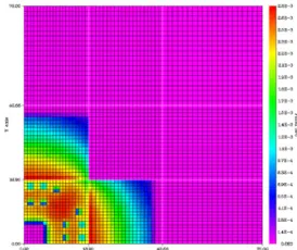
Figure 1. Meshing and material distribution used in the core level of VENUS2 TITAN model. Dosimeter locations are identified by ().
a. Source distribution, core axial-level b. 26-group source spectrum
0 5 10 15 20 25
0.00 0.02 0.04 0.06 0.08 0.10 0.12
Group
χg
Figure 2. VENUS-2 fixed-source specification.
4.1 TITAN Model
We have developed a 3-D model of the VENUS reactor using TITAN. The model consists of 8 axial-levels and a total of 17,775 fine meshes. Figure1shows the discretized model of the core level along with the 34 dosimeter locations (all of the dosimeters are located on the core midplane) with a numerical identification number for reference purposes. The reactor core is characterized by three homogenous regions: (1) an inner region with UO2 3.0 w/o enriched, (2) an outer region composed of UO2 4.0 w/o enriched, and (3) a MOX region with 2.0 w/o UO2 and 2.7 w/o Pu. Fast neutrons are of primary concern in this problem, therefore we will only consider neutron energies of 0.1 MeV or greater. The 26-group multigroup cross sections used are derived from the BUGLE-96 cross section library [6]. The 3-D fixed-source distribution used was generated from the data provided in the benchmark specification. Figure2a shows the source distribution at the core midplane and Fig.2b source spectrum.
4.2 Reference Solution Results
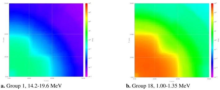
a. Group 1, 14.2-19.6 MeV b. Group 18, 1.00-1.35 MeV
Figure 3. 26-group reference solution flux distributions; normalized by the maximum flux in group 1.
Table 1. The upper energies of the first 26 groups of BUGLE-96.
Upper E Upper E Upper E Upper E Upper E
g [MeV] g [MeV] g [MeV] g [MeV] g [MeV]
1 19.60 7 6.07 13 2.37 19 1.00 25 0.30
2 14.20 8 4.97 14 2.35 20 0.82 26 0.18
3 12.20 9 3.68 15 2.23 21 0.74
4 10.00 10 3.01 16 1.92 22 0.61
5 8.61 11 2.73 17 1.65 23 0.50
6 7.41 12 2.47 18 1.35 24 0.37
in group 1, reference solution flux spectrum for groups 1 and 18; since the source spectrum peaks at energy group 18 the neutron flux in the core also peaks in this group, between 1.00 and 1.35 MeV.
The model was run on a single processor allocated with 8GB of memory; the TITAN calculated reference solution required∼110 seconds of computation time.
5. Testing TITAN-SDM
TITAN-SDM is tested with different coarse-group structures and the effects of algorithm control parameters are investigated. Table 1 presents the upper energy bounds of the 26-group structure of BUGLE-96.
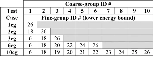
Table2presents the different coarse-group structures that are tested as identified by the fine-group number that defines the boundary of the coarse-group. The 2cg and 3cg structures were selected based on the energy structure of the BUGLE-96 library. The 4cg, 6cg, 8cg, and 10cg structures were selected by observing trends of the 26-group material cross sections; in areas of strong cross-section gradients more coarse groups were considered. New algorithm control parameters were introduced to check the convergence of coarse-group cross-section and coarse-group flux tolerance.
First, an analysis of the solution accuracy is presented through dosimeter reaction rate ratio,r, as compared to the standard multigroup TITAN. This ratio is given as
r= (RD)T I T AN−SDM (RD)Ref.
, (9)
where
RD =G
Table 2. Coarse-group testing structures.
Coarse-group ID # Test
Case
1 2 3 4 5 6 7 8 9 10
Fine-group ID # (lower energy bound)
1cg 26
2cg 18 26
3cg 6 18 26
6cg 6 18 20 22 24 26
10cg 6 18 19 20 21 22 23 24 25 26
Table 3. Analysis of the effect of coarse-group structures on solution accuracy and timing.
Case
58Ni 103Rh 237Np 27Al Time
RMS1 MAX2 RMS MAX RMS MAX RMS MAX [s]
1cg 0.9999 0.9994 0.9998 0.9993 0.9999 0.9990 0.9999 0.9992 658.8 2cg 0.9994 0.9984 0.9992 0.9978 0.9993 0.9980 0.9997 0.9990 578.7 3cg 0.9997 0.9989 0.9997 0.9992 0.9998 0.9990 1.0000 0.9992 650.7 10cg 0.9996 0.9984 0.9991 0.9958 0.9994 0.9973 1.0000 0.9992 738.7 1
Root-mean-squared value of dosimeter ratio,2maximum dosimeter ratio.
Table 4. Analysis of the effect of coarse-group flux tolerances on solution accuracy and timing for a 3 coarse-group structure.
Flux Tol. 58Ni 103Rh 237Np 27Al Time [s]
RMS1 MAX2 RMS MAX RMS MAX RMS MAX
10−3 0.9997 0.9989 0.9997 0.9992 0.9998 0.9990 1.0000 0.9992 650.7 10−2 0.9997 0.9989 0.9996 0.9980 0.9997 0.9988 1.0000 1.0007 620.5 10−1 1.0008 1.0017 0.9980 0.9812 1.0002 0.9946 1.0002 1.0020 627.9 1
Root-mean-squared value of dosimeter ratio,2maximum dosimeter ratio.
RDis the detector response,g,Dis the groupgdetector of typeDcross-section, andgis the fine-group scalar flux.
Reaction rates are calculated at each of the 34 positions, Fig. 1, for the following 4 dosimeter reaction types:58Ni(n,p),103Rh(n,n),237Np(n,f), and27Al(n,). Maximum absolute dosimeter ratio discrepancy and root-mean-squared (RMS) values are examined for each reaction type. Then, a detailed break down of times required for the different steps of the algorithm is discussed to identify areas for possible improvement.
5.1 Accuracy Analysis
Table 3 shows results of testing the different coarse-group structures, see Table 1, on the solution accuracy as well as computation time. For each coarse group, the maximum detector reaction rate ratio and root-mean-squared value are presented along with computation time. The fine-group flux is converged to 10−1and the coarse-group fluxes have either converged to 10−3or have met the maximum number of iterations allowed per subgroup iteration; this value is set to 10 iterations for all cases.
Table3demonstrates that number of coarse-group groups as well as selection of group boundaries has some impact on the accuracy of the calculation and the amount of computation time required. The fastest computation time is the 2cg case. The results indicate that the 3cg test case is the most accurate, showing the smallestrvalues.
Table 5. Total number of iterations for multigroups and SDM transport calculations.
Reference Multigroup SDM
(26 groups) (3 coarse groups)
324 134*
*Comprised of 122 coarse-group and 12 fine-group calculations.
Table 6. Fractional computation times1required for different steps of the TTIAN-SDM algorithm.
Coarse-group Fine-group Related
Transport Calculations
Total Source Total Source
0.27 0.22 0.73 0.60
1Total subgroup iteration time is 85.3 seconds.
Table4 indicates that, as expected, using a tighter coarse-group flux tolerance will produce more accurate reaction rates at the expense of computation time. As the flux tolerance is decreased, the accuracy of dosimeter reaction rates also decreases; the computation time also decreases slightly.
It should be noted that the required computation time for these TITAN-SDM calculations require significantly more, by nearly five times, computation time than the standard multigroup approach.
5.2 Analysis of Timing
Table5presents a comparison of the total number of transport calculations that are completed in the reference multigroup calculation and SDM algorithm. The SDM calculation total is broken down into the number of coarse-group transport calculations and fine-group transport calculations.
Table5demonstrates that the TITAN-SDM transport calculation requires significantly fewer, by a factor of∼2.5, number of iterations than the standard multigroup calculation. So, the question remains: why is the measured computation time significantly larger for TITAN-SDM? To answer this question, we examine the amount of computation time spent in different segment of the TITAN-SDM.
The total time required for a single subgroup (SG) loop is comprised of the sum of each of the four steps, previously discussed in Sect. 3: (1) coarse-group (CG) transport, (2) fine-group (FG) decomposition, (3) fine-group flux-update, and (4) coarse-group cross-section generation (the time required for this step is negligible compared to the other steps). To simplify this discussion we will consider the time spent on coarse-group transport, Step 1, and the combined time spent on fine-group related calculations, Steps 2 and 3. Table6presents the times required for the different steps of asingle subgroup iteration.
Table 6 demonstrates that ∼70% of the total subgroup iteration time is spent in on fine-group related calculations, while the coarse-group transport only accounts for ∼30% of the iteration time. This analysis shows that a significant amount, approximately 70%, of the computational costs of the SDM algorithm, for this fixed source problem, are spent obtaining the detailed flux spectrum and not on the coarse-group transport. It is concluded that a major portion, nearly 80%, of the computation time in both the coarse-group transport and fine-group related calculations is spent calculating the source terms.
5.3 Discussion
Table 7. Number of coarse-group iterations per subgroup iteration.
Criticality Fixed-source
600 30
calculations per subgroup iteration for the 1-D HTTR calculation [4] and the fixed-source problem presented here.
Table 7 shows that there are significantly more, nearly 20 times, coarse-group calculations per subgroup iteration for the criticality problem than there are for the fixed-source calculation. This analysis implies that the fixed-source calculation presented here is not computationally efficient because not enough coarse-group calculations are completed within a subgroup iteration. Hence, it is essential to explore development of more efficient calculations of determination a fine-group source using the coarse-group results.
6. Conclusions
In this paper we have tested the TITAN-SDM algorithm for fixed-source shielding application on the VENUS-2 benchmark problem. The SDM algorithm is shown to accurately calculate dosimeter responses. TITAN-SDM is sensitive to the number of coarse-groups selected and the definition of the coarse-group boundaries. It has been shown that in spite of significant reduction of number of transport sweeps, currently TITAN-SDM requires significantly more computation time than standard multigroup transport; the majority, ∼60%, of this time is spent on source calculation for the fine-group decomposition loop. The speedups observed in the criticality calculations are not observed for this fixed-source problem. We believe that this finding can be attributed to the small number of coarse-group transport calculations for a fixed-source calculation. Efforts are underway to explore alternative approaches for reducing the computation time used for source calculations.
The authors thank Drs. Saam Yasseri and Ce Yi and Profs. Farzad Rahnema and Glenn Sjoden of the Georgia Institute of Technology for their comments and suggestions.
References
[1] S. Douglass, F. Rahnema, Annals of Nuclear Energy48, 84 (2012) [2] S. Douglass, F. Rahnema, Annals of Nuclear Energy40, 200 (2012) [3] C. Yi, A. Haghighat, Nuc. Sci. Eng.164, 3 (2010)
[4] N. Roskoff, W. Walters, A. Haghighat, C. Yi, G. Sjoden, PHYSOR (2014), accepted [5] C.Y. Han, C. Shin, H.C. Kim, J.K. Kim,N. Messaoudi, B.C. Na, NEA/NSC/DOC(2004) [6] E. White, Oak Ridge National Laboratory, D00185-ALLCP-00 (1996)
[7] G. Bell, S. Glasstone,Nuclear Reactor Theory(Krieger Publishing Company, 1970) [8] S. Douglass, Ph.D. thesis, Georgia Institute of Technology (2012)