A Multi-Objective Collection-Distribution Center Location and Allocation Problem in a Closed-Loop Supply Chain for the Chinese Beer Industry

A Multi-Objective Collection-Distribution Center

Location and Allocation Problem in a Closed-Loop

Supply Chain for the Chinese Beer Industry

Kai Kang, Xiaoyu Wang and Yanfang Ma *

School of Economics and Management, Hebei University of Technology, Tianjin 300401, China; [email protected]

* Correspondence: [email protected]; Tel.: +86-22-6043-5164

Abstract: Recycling waste products is an environmental-friendly activity that can bring benefits to accompany, saving manufacturing costs and improving economic efficiency. For the beer industry, recycling bottles can reduce manufacturing costs and reduce the industry’s carbon footprint. This paper presents a model for a multi-objective collection-distribution center location and allocation problem in a closed loop supply chain for the beer industry, in which the objective is to minimize total costs and transportation pollution. Uncertainties in the form of randomness and fuzziness are jointly handled in this paper to ensure a more practical problem solution, for which returned bottle sand unusable bottles are considered fuzzy random variables. A heuristic algorithm based on priority-based global-local-neighbor particle swarm optimization (pb-glnPSO) is applied to ensure reliable solutions for this NP-hard problem. A case study on a beer operation company is conducted to illustrate the application of the proposed model and demonstrate the priority-based global-local-neighbor particle swarm optimization.

Keywords:collection-distribution center; closed loop supply chain; fuzzy random variable; particle swarm optimization

1. Introduction

Due to resource scarcity and environmental concerns, responsible companies are beginning to pay attention to the future of the planet and the global environment. Recycling used products for remanufacturing is, therefore, becoming of greater importance in supply chain management, a move that can dramatically reduce carbon emissions [1]. Closed loop supply chains (CLSC) combine the forward supply chain with a reverse supply chain that covers the whole life cycle of the products [2], with the manufacturing of new products and the transportation to customers via distribution centers and retailers as the forward supply chain and recycling, sorting, disposal and remanufacturing as the reverse supply chain. In recent years, the CLSC has received a great deal of academic and business attention because of the need to be socially responsible, environmental concerns and government legislation [3,4], which has motivated companies to pay more attention to recycling to reduce costs and lessen their carbon footprint.

transportation and inventory quantities on a CLSC network in the fashion industry. Khatami [10] proposed a scenario-based stochastic mixed-integer linear programming model to solve a CLSC network design problem, in which the retailers’ demand and the quantity of returned products were considered to be uncertain and the DC and CC were set. Vahdani [11] proposed capacitated bidirectional facilities to conduct distribution in a CLSC, in which a multi-priority queuing system was studied. Kim [12] designed a model to minimize the manufacturer’s total cost to find the optimal solution to the supply of raw material, the quantity of products and materials to be recycled, the recycling facility scale and the potential benefits or downfalls of joining a recycling association. As a growing number of companies are now engaging in recycling activities due to economic and environmental concerns, distribution and collection activities using the same vehicle has been found to reduce carbon emissions and transportation costs because empty loads can be avoided. In this paper, we combine the distribution center (DC) with the collection center (CC) as a collection-distribution center (CDC), which can benefit company operations and reduce construction costs. In practice, as the recycled product owners are usually at the same location as the potential new product buyer [13], a DC/CC combination requires less construction and operating expense sand can significantly reduce environmental pollution.

Ramkumar [14] developed a multi echelon, multi period, multi product closed loop supply chain network model which was solved using a genetic algorithm with fixed variables. Kaya and Onur [13] presented a facilities location-inventory-pricing model without uncertainty to determine the optimal location for facilities. Barz [15] proposed an optimization model for a two-stage capacitated facilities location and allocation problem with the effects of additive manufacturing, in which all the variables were certain. Jindal [16] developed a multi-objective model for a CLSC network design problem that considered the economic and environmental factors as fuzzy uncertain and in which the DC and CC were separate. Ramezani [17] conducted research into a CLSC network design problem that only considered fuzzy variables. In recent years, uncertainty has attracted more research attention [18–20]. Stochastic programming, robust optimization, and fuzzy set theory are three applicable tools which can be used to present uncertainty in the FLAP [21,22]. Keyvanshokooh [23] proposed a novel hybrid robust-stochastic programming (HRSP) approach to simultaneously model two different types of uncertainties by including stochastic scenarios for transportation costs and polyhedral uncertainty sets for demands and returns. However, they considered the DC and the CC to be separate and the collection disposal rate was treated as a certain variable. Uncertainties exist in both the forward supply and reverse supply chains; however, the uncertainties in the reverse flow are higher than those in the forward supply chain [7,19], with the returned product quantity generally being considered uncertain [10,23]. Subjective uncertainties such as decision maker’s choices and the environmental coefficients can be dealt with using fuzziness and objective uncertainties such as unit transportation costs, product prices and the quantity of unusable products can be dealt with using randomness. In this paper, the return rate and disposal rate are considered fuzzy random variables to reflect the problem. The random and fuzzy uncertainties are handled together and represented by triangular fuzzy numbers [7]. Based on the above consideration, the model is formulated to determine the proper number and location of the CDCs as well as the allocation strategy between the different kinds of facilities.

random simulation-based bi-level global-local-neighbor particle swarm optimization (frs-bglnPSO). In this paper, a priority-based global-local-neighbor particle swarm optimization (pb-glnPSO) is applied to solve the CDCLAP.

In summary, this paper proposes a multi-objective model to solve a collection-distribution center location and allocation problem in a closed loop supply chain that considers the economic and environmental factors and includes fuzzy random variables for the return and disposal rates. The remainder of this paper is organized as follows: Section2presents the problem statement and model assumptions. A description of the model and its formulation are given in Section3. The proposed hybrid solution based on the pb-glnPSO is described in Section 4. A case study is conducted to illustrate the model formulation and the proposed method in Section5. Finally, Section6concludes this paper.

2. Research problem statement

In this paper, a company with factories at certain locations and several retailers at different customer zones are considered. The company is considering whereto set the integrated collection and distribution centers (CDC), at which both the collection network for used products and the distribution network for new products are jointly established [13]. CDCs reduce both construction and transportation costs because the same vehicles can be used for both distribution and recycling. Therefore, in this paper, only CDCs are considered.

 

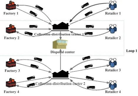
Figure 1.The closed loop supply chain network

A general illustration of the classical CDCLAP for a closed loop supply chain is shown in Fig1, with the CLSC framework shown in loop1. The CLSC framework has four echelons: factories, CDCs, retailers and disposal centers [11]. The forward supply chain begins with new production. From the factories, the finished products are transported to the retailers via the CDCs. In the reverse supply chain, the returned products are collected and transported to the CDCs, where the recycled products are inspected, consolidated and sorted into those that are available for remanufacturing, which are sent to the factories, and those that are unsuitable for remanufacturing, which are transported to the disposal centers [23]. A CDC can supply products to multiple retailers and retailer demand is fulfilled by only one production site. A CDC can handle products from different factories and send the returned products to multiple factories for remanufacturing.

between two facilities. Another fuzzy random variable considered in this paper is the returned product disposal rate, which is decided on after inspection and consolidation at the CDC.

Following are the assumptions in the proposed problem investigation: (1) Only one product one period is considered; (2) All alternative locations for the CDCs have been identified; (3) Recycling a used product costs less than manufacturing a new one [31]; (4) Considering uncapacitated facilities is an unrealistic assumption in many LAP problems. Many researchers assign a maximum capacity level to facilities to model more realistic decisions. The CDCs and the factories have a capability limit [32–34]; (5) The locations for the factories, retailers and disposal centers are known; (6) New product and returned product storage is allowed at the CDCs [22].

The initial problem is making a decision as to where to set the CDCs from the candidate sites and deciding on an allocation strategy at minimal total CDC costs; operating costs, transportation costs and transportation pollution cost; while also considering the flow constraints, capability limits and the retailers’ demand.

3. Modelling

In this section, a mathematical description is given for the CDCLAP in the CLSC, including the notations, the research problem statement, and the mathematical formulation.

3.1. Notations

To facilitate the problem description, the notations are explained. Sets

Ω: set of CDCs,Ω={1, 2, 3, ...,I}. Ψ: set of factories, andΨ={1, 2, 3, ...,J}

Φ: set of retailers, andΦ={1, 2, 3, ...,K}

Υ: set of disposal centers, andΥ={1, 2, 3, ...,N}

Indices and parameters

i: alternative location position for the CDCs,i∈Ω={1, 2, 3, ...,I}. j: known position of the factories,j∈Ψ={1, 2, 3, ...,J}.

k: known position of the retailers,k∈Φ={1, 2, 3, ...,K}. n: known disposal center,n∈Υ={1, 2, 3, ...,N}. U: the upper limit of the CDCs.

Dk: the demand of retailerk. αi: the capability of CDCi. γj: the capability of factoryj.

Pji: product quantity from factoryjto CDCi. Qik: product quantity from CDCito retailerk.

ea_k: the product return rate from retailerk. ebi: the product disposal rate at CDCi. F_ic: the fixed costs of the CDC.

V_ic: the variable cost of the CDC for a new product unit. RVc

i: the variable cost of the CDC triage for a returned product unit. C_ijp: unit transportation cost between CDCiand factoryj.

Cd

ik: unit transportation cost between CDCiand retailerk.

Cw_in: unit transportation cost between CDCiand disposal centern. βij: environmental impact of transportation between CDCIand factoryj. βik: environmental impact of transportation between CDCiand retailerk.

Decision variables

xi: a binary variable indicating whether pointiis chosen. If pointiis chosen, thenxi =1; else,xi=0.

yik: indicates whether retailerkis served by CDCi. Ifiis chosen, thenyik=1; else,yik=0.

3.2. Objective functions

A multi-objective DCCLAP model using the above variables is proposed to minimize total costs and the environmental transportation effects.

Economic objective: In general, decision makers seek to minimize the total costs, which are made up of the transportation costs, fixed costs and operating costs. The minimization objective can be described as

minZ1=

I

∑

i=1 J

∑

j=1 C_ijpPji+

I

∑

i=1 K

∑

k=1

C_ikdQ_ik(1+ea_k) +

I

∑

i=1 N

∑

n=1 K

∑

k=1 C_inweb

iea_kQ_ik+

I

∑

i=1 J

∑

j=1 K

∑

k=1 N

∑

n=1

C_ijpea_kQ_ik(1−ebi)

+

I

∑

i=1 F_icXi+

I

∑

i=1 J

∑

j=1 V_icPji+

I

∑

i=1 K

∑

k=1

RV_icea_k (1)

Equation (1) calculates the total cost, in which∑I_i=1∑_jJ₌₁C_ijpPji represents the cost of new product transported from factories to CDC, ∑I_i=1∑K_k=1C_ikdQik(1+eak) calculated the transportation cost between CDCs and retailers,∑I

i=1∑nN=1∑Kk=1Cwinebiea_kQ_ikis the cost of returned product delivered from CDCs to disposal centers as well as the returned product transportation cost from CDCs to disposal centers is measured as∑I

i=1∑ J j=1∑

K

k=1∑nN=1C p

ijea_kQ_ik(1−ebi). The fixed cost of opening a new CDC is presented as∑I

i=1FicXi. ∑iI=1∑ J

j=1VicPjishows the variable cost of new product. ∑Ii=1∑Kk=1RVicea_k calculates the operation cost of returned product.

It is very difficult to handle the objective function with fuzzy random factors. Kruse and Meyer [35] point out that the fuzzy expected value may be represented by a single fuzzy number. Without a loss of generality, based on the theory proposed by Heilpern [36], the expected value operator is used to enable the conversion of the uncertain model into the deterministic. Now the fuzzy random objective function can be transformed into their crisp equivalences as shown in Eq. (2):

minZ1=

I

∑

i=1 J

∑

j=1 C_ijpPji+

I

∑

i=1 K

∑

k=1

Cd_ikQik(1+EV[ea_k]) +

I

∑

i=1 N

∑

n=1 K

∑

k=1

C_inwEV[eb_i]EV[_ea

k]Qik

+ I

∑

i=1 J

∑

j=1 K

∑

k=1 N

∑

n=1

C_ijpEV[ea_k]Q_ik(1−EV[eb_i]) +

I

∑

i=1 F_icXi+

I

∑

i=1 J

∑

j=1 V_icPji+

I

∑

i=1 K

∑

k=1

RV_icEV[ea_k] (2)

Note theEV[ea_k]orEV[eb_i]above represents two expected values: the first one being the fuzzy random variables converted into fuzzy numbers based on the theory proposed by Kruse and Meyer in 1987, and the second being used to transform the fuzzy numbers into deterministic numbers based on the theory proposed by Heilpern in 1992.

minZ2= I

∑

i=1 J

∑

j=1

βijPji+ I

∑

i=1 K

∑

k=1

βikQik(1+EV[ea_k]) +

I

∑

i=1 N

∑

n=1 K

∑

k=1

βinEV[eb

i]EV[ea_k]Q_ik

+ I

∑

i=1 J

∑

j=1 K

∑

k=1 N

∑

n=1

βijEV[ea_k]Q_ik(1−EV[eb_i]) (3)

∑I i=1∑

J

j=1βijPji refers to the environment pollution caused by transportation activities from factories to CDCs. ∑I

i=1∑Kk=1βikQik(1+EV[ea_k]) is the summation of carbon footprints when transporting products between CDCs and retailers.∑_iI₌₁∑_nN₌₁∑K_k=1βinEV[eb_i]

EV[ea_ki]Q_ik is the total carbon footprint from CDCs to disposal centers. And ∑I

i=1∑ J

j=1∑Kk=1∑nN=1βijEV[ea_k]Q_ik(1−EV[eb_i])express the carbon footprints from CDCs to factories when delivering returned products.

3.3. Constraints

Note that the CDC has its own capacity limit and it cannot service any goods beyond its capacity. Thus we need capacity restriction. The constraint can be written as follows:

K

∑

k=1

EV[ea_k]Q_ik+ J

∑

j=1

Pji≤αi ∀i∈Ω (4)

f

akiis a fuzzy random variable indicating the return rate of the used product to transport from retailer

kto CDCi. Qikshows product quantity from CDCi to the retailerk. Pji indicates the quantity of

product to transport from factoryjto CDCi.αirefers to the capacity of the the capability of the CDC

i.

As for capability constraint, the factory can manufacturing the new products that the retailers need and the returned products send back by CDCs.

K

∑

k=1

Dk+ I

∑

i=1

K

∑

k=1

N

∑

n=1

C_ijpEV[eak]Qik(1−EV[eb_i])≤ J

∑

j=1

γj (5)

Dk refers to the demand of retailer k and γj is the capability of the factory j. ∑I

i=1∑Kk=1∑Nn=1C p

ijEV[ea_k]Q_ik(1− EV[eb_i]) calculates the returned product transported to factory jfor remanufacture.

Considering the products in the retailers are all from the CDCs, the recycled products are less than the product transported from factory to the CDC And it can be described as follows:

J

∑

j=1

Pji≥ K

∑

k=1

EV[ea_k]Q_ik (6)

Pjiis a variable indicating the quantity of new product transported from the factoryjto CDCi.ae_kQ_ik refers to the quantity of returned product transported from retailerkto CDCi.

The product provided to the retailer should at least meet the retailer’s demand.

I

∑

i=1

Qik≥ K

∑

k=1

Dk (7)

Qikindicates the product quantity CDCito the retailerk. the stochastic variableDkis the demand of

The returned products transported to the CDCs are more than the products transported to the disposal centers.

K

∑

k=1

EV[ea_k]Q_ik≥ N

∑

n=1

K

∑

k=1

EV[eb_i]EV[_ea_k]Q_ik (8)

EV[ea_k]Q_ikis the expression of returned product quantity from the retailerkto CDCi,EV[eb_i]EV[ea_k]Q_ik presents the product quantity transported from CDCito retailerk.

The CDC should be at least one but no more than the upper limit.

1≤

I

∑

i=1

xi (9)

I

∑

i=1

xi≤U (10)

U is the upper limit of the CDCs, which is decided by the demand, the returned product quantity and the fixed capability.

It should make sure that each retailer is served by one CDC.

I

∑

i=1

yik=1 (11)

Sincexiandyikare binary variables, the following constraints are needed:

xi ={0, 1}, ∀i∈Ω, (12)

yik={0, 1}, ∀i∈Ω, ∀k∈Φ (13)

xiis a binary variable indicating whether a CDC is opened at pointi. If locationiis chosen to open a CDC, thenxi =1; otherwise,xi=0.yikis a binary variable indicating whether retailerkis served by CDCi. Ifyik=1, then retailerkis served by CDCi; otherwise,yik=0.

3.4. Global model

minZ1= I

∑

i=1 J

∑

j=1 C_ijpPji+

I

∑

i=1 K

∑

k=1

C_ikdQik(1+EV[ea_k]) +

I

∑

i=1 N

∑

n=1 K

∑

k=1

Cw_inEV[eb

i]EV[ea_k]Q_ik

+ I

∑

i=1 J

∑

j=1 K

∑

k=1 N

∑

n=1

C_ijpEV[ea_k]Q_ik(1−EV[eb_i]) +

I

∑

i=1 F_icXi+

I

∑

i=1 J

∑

j=1 V_icPji+

I

∑

i=1 K

∑

k=1

RV_icEV[ea_k]

minZ2=

I

∑

i=1 J

∑

j=1

βijPji+ I

∑

i=1 K

∑

k=1

βik(Qik+EV[ea_k]) +

I

∑

i=1 N

∑

n=1

βinEV[eb

i] + I

∑

i=1 J

∑

j=1 K

∑

k=1 N

∑

n=1

βij(EV[ea_k]−EV[eb_i])

s.t.                                                                            K ∑ k=1

EV[ea_ki]Q_ik+

J

∑

j=1

Pji≤αixi ∀i∈Ω ∀j∈Ψ ∀k∈Φ

K

∑

k=1

Dk+∑iI=1∑Kk=1∑nN=1C

p

ijEV[ea_k]Q_ik(1−EV[eb_i])≤

J

∑

j=1

γj ∀j∈Ψ ∀k∈Φ ∀n∈Υ

J

∑

j=1

Pji≥

K

∑

k=1

EV[eaki] ∀i∈Ω ∀j∈Ψ ∀k∈Φ

K

∑

k=1

EV[ea_k]Q_ik≥

N ∑ n=1 K ∑ k=1 EV[eb

i]EV[ea_k]Q_ik ∀i∈Ω ∀k∈Φ ∀n∈Υ

I

∑

i=1

Qik≥

K

∑

k=1

Dk ∀i∈Ω ∀k∈Φ

1≤ _∑I

i=1

xi ∀i∈Ω

I

∑

i=1

xi≤U ∀i∈Ω

yik≤xi ∀i∈Ω, ∀k∈Φ

I

∑

i=1

yik=1 ∀i∈Ω ∀k∈Φ

xi={0, 1} ∀i∈Ω,

yik={0, 1} ∀i∈Ω, ∀k∈Φ

(14)

4. The heuristic algorithms based on Pgln-PSO

Particle swarm optimization (PSO) is a recent evolutionary algorithm which simulates social behavior such as birds flocking and fish schooling [38]. The PSO searches the feasible zone to seek solutions using a fixed population of individuals, which are updated to achieve the optimal solution. The particles [39] are characterized by their position and velocity, which are decided on by their flying experience or discoveries or those of their companions. They fly through the problem spaces following the current optimum particles to find the best solution between the populations and the best solution for each population. The PSO has been widely used to solve NP-hard problems [38]. However, in the basic PSO, it was found that the particles in the swarm were weak and clustered rapidly toward the global best particle [25]. Global-local-neighbor particle swarm optimization (glnPSO) proposed by Ai and Kachitvichyanukul [30] improves the weakness of the basic PSO. Xu and Yan [40] proposed a global-local-neighbor particle swarm optimization with exchangeable particles (GLNPSO-ep), which was even more advanced. In this section, a priority-based global-local-neighbor particle swarm optimization (pb-glnPSO) is proposed to solve the multi-objective CDCLAP in the CLSC.

4.1. Notations for the Pb-glnPSO

τ: iteration index, andτ=1, 2, ...T. d: dimension index, andd=1, 2, ...D. l: particle index, andl=1, 2, ...L. ωτ: inertia weight inτ−thiteration.

vld(τ): velocity of thelth particle at thedth dimension in theτth iteration. pl_d(τ): position of thelth particle at thedth dimension in theτth iteration. pbest_ld : personal best position.

pbest_gd : global best position. p_ldLbest: local best position. pNbest

ld : near neighbor best position.

cp: personal best position acceleration constant. cg: global best position acceleration constant. cl: local best position acceleration constant.

cn: near neighbor best position acceleration constant. Pmax: maximum position value.

Pmin: minimum position value. Pl: velocity vector ofl-th particle. Vl: position vector ofl-th particle.

P_lbest: vector personal best position ofl-th particle. Pgbest: vector global personal best position.

P_lLbest: vector local best position ofl-th particle.

r1,r2,r3,r4: uniform distributed random number within [0,1]. Fitness(Pl): fitness value ofPl.

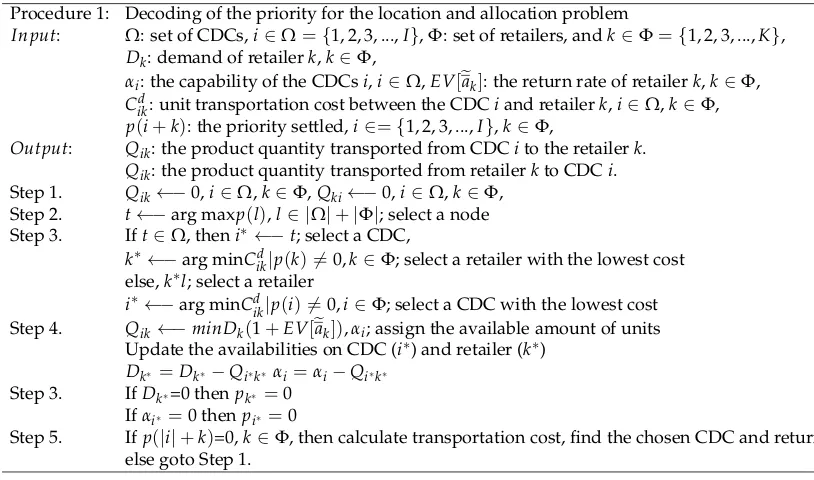
4.2. Encoding and decoding algorithm

Table 1.Decoding for the location and allocation problem

Procedure 1: Decoding of the priority for the location and allocation problem

Input: Ω: set of CDCs,i∈Ω={1, 2, 3, ...,I},Φ: set of retailers, andk∈Φ={1, 2, 3, ...,K},

Dk: demand of retailerk,k∈Φ,

αi: the capability of the CDCsi,i∈Ω,EV[ea_k]: the return rate of retailerk,k∈Φ,

Cd

ik: unit transportation cost between the CDCiand retailerk,i∈Ω,k∈Φ,

p(i+k): the priority settled,i∈={1, 2, 3, ...,I},k∈Φ,

Output: Qik: the product quantity transported from CDCito the retailerk.

Qik: the product quantity transported from retailerkto CDCi.

Step 1. Qik←−0,i∈Ω,k∈Φ,Qki←−0,i∈Ω,k∈Φ,

Step 2. t←−arg maxp(l),l∈ |Ω|+|Φ|; select a node Step 3. Ift∈Ω, theni∗ ←−t; select a CDC,

k∗ ←−arg minCd

ik|p(k)6=0,k∈Φ; select a retailer with the lowest cost

else,k∗l; select a retailer

i∗←−arg minCd

ik|p(i)6=0,i∈Φ; select a CDC with the lowest cost

Step 4. Qik←−minDk(1+EV[ea_k]),α_i; assign the available amount of units Update the availabilities on CDC (i∗) and retailer (k∗)

Dk∗=D_k∗−Q_i∗_k∗αi=αi−Qi∗_k∗ Step 3. IfD_k∗=0 thenp_k∗=0

Ifαi∗=0 thenp_i∗=0

Step 5. Ifp(|i|+k)=0,k∈Φ, then calculate transportation cost, find the chosen CDC and return, else goto Step 1.

4.3. Update

Based on the above notations and the glnPSO proposed by Ai and Kachitvichyanukul [30], the inertia weight, velocity and position are updated using the following Equation.

ω(τ) =ω(T) +τ−T

1−T[ω(1)−ω(T)] (15)

vl_d(τ+1) =ω(τ)vl_d(τ) +cpr1[pbestld (τ)−pld(τ)] +cgr2[pbestgd (τ)−pld(τ)] +clr3[pbestgd (τ)−pld(τ)]

+cnr4[pbestgd (τ)−pld(τ)] (16)

pl_d(τ+1) = pl_d(τ) +vl_d(τ+1) (17)

1 Z

2 Z

) ( ）

（Pl FitnessPgbest

Fitness 

) ( ）

（Pl FitnessPlbest

Fitness 

l best

l P

P 

l best _P

Pg 

Lbest

Pl

Nbest ld P

 

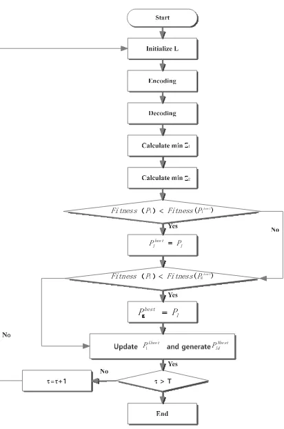
Figure 2.The heuristic algorithms based on pb-glnPSO

4.4. Overall process of the pb-glnPSO

In this paper, the glnPSO presented above is used to solve the location and allocation problem. Due to uncertainties and environmental changes, a priority-based global-local-neighbor particle swarm optimization (pb-glnPSO) is proposed to solve this model. As the company pays close attention to the economic costs, the environmental factor is dealt with as a constraint which has upper limits. The algorithmic details are as follows.

Step 1: Initialize P particles as a swarm:l=1, ...L, (the particle is the priority).

Step 2: Constraints check. If in the feasible region, goto step 3; otherwise, return to step 1. Step 3: Calculate the fitness according to the decoding algorithm in Table1.

Step 4: Update the particle positions and velocities.

Step 4.1: Acquire the expected value forZfrom the above algorithm.

Step 4.2: Forl =1, 2, ...L, decode each particle to an installment group. Calculate the fitness value of each particle and set as the position of the l-th particle as its personal best. The global best position is chosen from these personal best positions.

Step 4.3: Update pbest: Forl=1, 2, ...L, ifFitness(Pl)<Fitness(Plbest),Plbest=Pl. Step 4.4: Update gbest: Forl=1, 2, ...L, ifFitness(Pl)<Fitness(Pgbest),Pgbest=Pl.

Step 4.5: Update lbest: For l = 1, 2, ...L, among all pbest of M neighbors around the l-th particle, set the personal best which has the best fitness value asP_lLbest.

Step 4.6: Generate nbest: Forl=1, 2, ...L, andd=1, 2, ...D, find thepodensuring that the FDR takes a maximum value, and setpodasPldNbest.

Step 4.7: Update the position and the velocity of each l-th particle using Equation (18). Step 4.8: Check whether the particles are beyond the mark. If pld > Pmax, the pld = Pmax; otherwise, ifpld <Pmin, thennpld =Pmin.

Step 6: If the stopping criterion is met, stop; otherwise,τ=τ+1 and return to step 2. The overall process can be clearly seen in Fig2.

5. Case Study

5.1. Case presentation

This model is motivated by a beer company in a developing country that bottles beer in plastic or glass bottles. The supply chain intends to allow customers to return the bottles to the retailers after the beer has been consumed, after which the returned bottles are sent to the CDCs where they are inspected, consolidated and sorted. After processing and disinfecting, the bottles are filled with beer and sold again. Now the company is considering the construction of several CDCs to allow for bottle recycling as producing a new bottle is far more expensive than recycling a used bottle.

Table 2.CDCs information (unit:1×102RMB)

Node location capability fixed cost NPV cost RPV cost eb

i Parametersρ

1 (23,23) 900 12300 0.01 0.05 (0.18,ρ₁,0.25) ρ₁∼N(0.21,0.02)

2 (25,35) 550 12100 0.02 0.06 (0.23,ρ₂,0.28) ρ₂∼N(0.25,0.02)

3 (34,29) 1050 15600 0.01 0.05 (0.14,ρ₃,0.24) ρ₃∼N(0.18,0.04)

4 (32,25) 650 11300 0.01 0.07 (0.16,ρ₄,0.22) ρ₄∼N(0.18,0.03)

5 (35,37) 1050 17800 0.01 0.05 (0.25,ρ₅,0.30) ρ₅∼N(0.28,0.02)

6 (36,31) 1050 22400 0.01 0.06 (0.17,ρ₆,0.26) ρ₆∼N(0.22,0.03)

7 (29,28) 1050 16300 0.02 0.07 (0.15,ρ₇,0.23) ρ₇∼N(0.20,0.02)

8 (18,21) 800 14900 0.01 0.06 (0.19,ρ₈,0.28) ρ₈∼N(0.24,0.03)

9 (29,23) 1100 26500 0.01 0.06 (0.12,ρ₉,0.22) ρ₉∼N(0.17,0.04)

10 (35,26) 1050 22000 0.02 0.05 (0.17,ρ₁₀,0.23) ρ₁₀∼N(0.20,0.02)

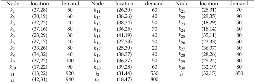
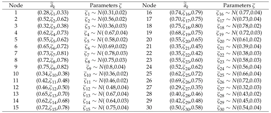
To illustrate the validity of the model and the usefulness of the solution method, the data needed to examine the CLSC performance for the four objectives is presented here. Based on the market analysis, ten coordinates for the CDC alternatives are given: location, capability, fixed costs and new product variable costs (NPV cost) and recycled product variable costs (RPV cost). These are shown in Table2. Supermarkets and restaurants are considered to beer tailers with flexible demand. Table3presents the information regarding the retailers, factories and disposal centers. It can be seen from that Table3,k1tok30 represents 30 different retailers, whilej1toj4are the 4 different factories at different locations with variable capabilities and n1 indicates the location and capability of the disposal center. Therefore, 30 retailers, 4 factories and 1 waste disposal center are considered in this study. The unit transportation costs and pollution are related to the distances between the facilities. The retailers’ return rates are shown in Table4, which are considered to be fuzzy random variables.

Table 3.Rtailers, factories and disposal center

Node location demand Node location demand Node location demand

k1 (27,28) 50 k11 (26,39) 60 k21 (25,31) 70

k2 (30,19) 60 k12 (38,26) 40 k22 (29,35) 90

k3 (32,22) 40 k13 (38,34) 50 k23 (18,29) 50

k4 (37,16) 80 k14 (36,25) 70 k24 (18,14) 60

k5 (23,29) 30 k15 (41,19) 40 k25 (35,11) 80

k6 (27,17) 40 k16 (27,33) 30 k26 (23,33) 50

k7 (33,26) 80 k17 (25,39) 20 k27 (36,37) 60

k8 (34,32) 40 k18 (38,37) 40 k28 (28,26) 40

k9 (37,22) 100 k19 (36,27) 50 k29 (25,24) 30

k10 (17,22) 90 k20 (39,28) 60 k30 (32,19) 80

j1 (13,22) 920 j2 (31,44) 530 j3 (32,15) 850

Table 4.Retailers’ return rates and CDCs’ disposal rate

Node ea_k Parametersς Node ea_k Parametersς

1 (0.28,ς1,0.33) ς1∼N(0.31,0.02) 16 (0.74,ς16,0.79) ς16∼N( 0.77,0.04)

2 (0.52,ς₂,0.62) ς₂∼N(0.56,0.02) 17 (0.70,ς₁₇,0.75) ς₁₇∼N(0.73,0.04)

3 (0.32,ς3,0.38) ς3∼N(0.36,0.03) 18 (0.75,ς18,0.80) ς18∼N(0.78,0.02)

4 (0.62,ς₄,0.73) ς₄∼N( 0.67,0.04) 19 (0.68,ς₁₉,0.75) ς₁₉∼N( 0.72,0.03)

5 (0.55,ς5,0.62) ς5∼N( 0.58,0.02) 20 (0.55,ς20,0.65) ς20∼N(0.61,0.02)

6 (0.65,ς₆,0.72) ς₆∼N(0.69,0.02) 21 (0.35,ς₂₁,0.45) ς₂₁∼N(0.39,0.04)

7 (0.73,ς₇,0.81) ς₇∼N( 0.78,0.03) 22 (0.35,ς₂₂,0.42) ς₂₂∼N(0.38,0.03)

8 (0.72,ς8,0.78) ς8∼N(0.75,0.03) 23 (0.55,ς23,0.60) ς23∼N(0.58,0.03)

9 (0.75,ς₉,0.82) ς₉∼N(0.8,0.04) 24 (0.52,ς₂₄,0.62) ς₂₄∼N(0.56,0.04)

10 (0.34,ς10,0.38) ς10∼N(0.36,0.02) 25 (0.62,ς25,0.72) ς25∼N(0.66,0.04)

11 (0.42,ς₁₁,0.48) ς₁₁∼N(0.46,0.02) 26 (0.69,ς₂₆,0.75) ς₂₆∼N(0.72,0.03)

12 (0.46,ς12,0.50) ς12∼N( 0.48,0.04) 27 (0.29,ς27,0.35) ς27∼N(0.32,0.03)

13 (0.65,ς₁₃,0.70) ς₁₃∼N( 0.67,0.04) 28 (0.40,ς₂₈,0.46) ς₂₈∼N(0.43,0.02)

14 (0.62,ς₁₄,0.68) ς₁₄∼N( 0.64,0.03) 29 (0.42,ς₂₉,0.48) ς₂₉∼N(0.45,0.03)

15 (0.72,ς15,0.78) ς15∼N( 0.75,0.04) 30 (0.50,ς30,0.58) ς30∼N(0.54,0.04)

5.2. Sensitivity analysis on the parameters

To find the best solution to the proposed model, a series of experiments were conducted, all of which were performed using a MATLAB 7.0 on a workstation with an Intel(R) Corei5, a Pentium 4, 1.83GHz clock pulse with 4GB memory and Windows 10 operating system. A sensitivity analysis was performed to exhibit the effectiveness and behavior of the proposed algorithm, as shown in Table5. Several parameters were changed, including the population size N, maximum generation Tand acceleration constantcp,cg,clandcn. After trying various values for the population size and maximum generations, the results were found to be better whenTwas from 200 to 400 and Nwas from 30 to 50. The different fitness values obtained using the pb-glnPSO with the different parameters N T c1andc2are shown in Table5.

Table 5.Sensitivity analysis (unit:1×102RMB)

T=200 T=300 T=400 T=200 T=300 T=400 T=200 T=300 T=400

0.5 88049.270 85447.261 86943.479 89889.371 88266.237 84859.596 86479.923 84830.640 88233.839 1 87056.401 84125.454 84428.258 88679.314 87459.033 84199.470 85596.767 83448.794 85614.352 1.5 86601.808 84465.348 84315.569 85486.560 86564.333 84041.957 84698.625 83257.776 82930.618 2 85614.087 82308.935 83058.532 82914.087 82434.420 83681.801 82884.954 81920.133 82585.367 2.5 85844.692 83102.944 87782.377 85170.526 83198.452 86792.664 83448.789 84469.925 83177.298

As can be seen from Table5, when the parameterscp, cg,cl and cn increase, the fitness value improves except forcp=cg=cl=cn=2.5 with the same generation and popsize, with the fitness value increasing from cp=cg=cl=cn=2 tocp=cg=cl=cn=2.5. Therefore, when cp=cg=cl=cn=2, the result is optimal. For T, given the samecp, cg,cl and cn and population size, the results shows that when Tis 300, the fitness value is better than for any other generation. Finally, forN, the results improve as the population size increases and is optimal whenNis 50. The most effective and efficient results are gained withTat 300,Nat 50 andcp=cg=cl=cn=2.

5.3. Result analysis

10 15 20 25 30 35 40 45 10

15 20 25 30 35 40 45

Retailer CDC Factory Disposal center

You created this PDF from an application that is not licensed to print to novaPDF printer (http://www.novapdf.com)

Figure 3.The distribution strategy

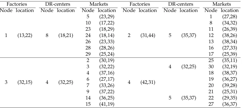
costs. The results are presented in Table6and Figure3. From the calculation, at least 3 CDCs could satisfy all markets. The result show that alternative CDC positions4, 5 and 8 should be chosen as CDC 4 can send products to markets 2, 3, 4, 6, 7, 9, 14, 15, 25, 30, CDC 5 can transport products for 1, 8, 11, 12, 13, 16, 17, 18, 19, 20, 21, 22, 27 and retailers 5, 10, 23, 24, 26, 28, 29 can be serviced by CDC 8. The total cost is 81.936million RMB, in which the fixed costs are 44 million RMB, the transportation costs are 37.759 million RMB and the operating costs are 17.7 million RMB.

Table 6.Results

Factories DR-centers Markets Factories DR-centers Markets

Node location Node location Node location Node location Node location Node location

1 (13,22) 8 (18,21) 5 10 23 24 26 28 29

(23,29) (17,22) (18,29) (18,14) (23,33) (28,26) (25,24)

2 (31,44) 5 (35,37) 1 8 11 12 13 16 17

(27,28) (34,32) (26,39) (38,26) (38,34) (27,33) (25,39)

3 (32,15) 4 (32,25) 2 3 4 6 7 9 14 15

(30,19) (32,22) (37,16) (27,17) (33,26) (37,22) (36,25) (41,19)

4 (42,31) 4

5

(32,25)

(35,37) 25 30 18 19 20 21 22 27

(35,11) (32,19) (38,37) (36,27) (39,28) (25,31) (29,35) (36,37)

5.4. Algorithm comparison

To better illustrate the effectiveness of the proposed algorithm, a brief comparison between the pb-glnPSO, glnPSO and an immune algorithm(IM) is given in this section. The glnPSO is a well-respected evolutionary algorithm and has been successfully implemented in a variety of engineering and combinatorial problems.The IM has also being widely used to solve facilities location problems.

wasω(1)=1 andω(T)=0.1. For the IM algorithm, the crossover probability was1 and the mutation probability was 0.1.

0 50 100 150 200 250 300

8 8.5 9 9.5 10 10.5 11 11.5x 10

4

Iteration

Fitness value function

0 50 100 150 200 250 300

8 8.5 9 9.5 10 10.5 11 11.5x 10

4

Iteration

F

it

n

e

ss

va

lu

e

f

u

n

ct

io

n

pb-glnPSO glnPSO IM

You created this PDF from an application that is not licensed to print to novaPDF printer (http://www.novapdf.com)

Figure 4.The iterative process of pb-glnPSO,glnPSO and IM

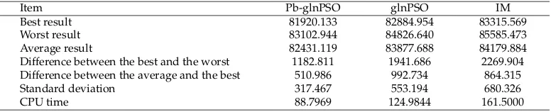
From Figure4, it can be seen that the pb-glnPSO outperformed both the glnPSO and the IM, and as the glnPSO converged faster, it had a better result than the IM. This demonstrates that a better solution can be obtained using the glnPSO, and especially using the pb-glnPSO. The blue profile shows the convergence for the best in history for the pb-glnPSO. It can be seen from Figure4that as the programs ran, the results become stable for the pb-glnPSO and glnPSO after about the 160th generation, while the IM became stable after the 180th generation. As is shown in Figure4, the best solution for the pb-glnPSO was superior to, more stable than and had the smallest CPU run time than the other algorithms( Table7), with the IM having the highest run time.

Table 7.Results of the pb-glnPSO, glnPSO, and IM

Item Pb-glnPSO glnPSO IM

Best result 81920.133 82884.954 83315.569

Worst result 83102.944 84826.640 85585.473

Average result 82431.119 83877.688 84179.884

Difference between the best and the worst 1182.811 1941.686 2269.904 Difference between the average and the best 510.986 992.734 864.315

Standard deviation 317.467 553.194 680.326

CPU time 88.7969 124.9844 161.5000

6. Conclusion

reuse policies. At the same time, the transportation costs and pollution were reduced because of the reduction in losses from empty loads.

References

1. Li, J.; Du, W.; Yang, F.; Hua, G. The Carbon Subsidy Analysis in Remanufacturing Closed-Loop Supply Chain.Sustainability2014,6(6), 3861-3877.

2. Ma, J.; Wang, H. Complexity analysis of dynamic noncooperative game models for closed-loop supply chain with product recovery.Applied Mathematical Modelling2014,38(23), 5562-5572.

3. Giri, B.C.; Sharma, S. Optimizing a closed-loop supply chain with manufacturing defects and quality dependent return rate.Journal of Manufacturing Systems2015,35, 92-111.

4. Rezapour, S.; Farahani, R.Z.; Fahimnia, B.; Govindan, K.; Mansouri, Y. Competitive closed-loop supply chain network design with price-dependent demands.Journal of Cleaner Production2015,93, 1-22.

5. Subramanian, P.; Ramkumar, N.; Narendran, T.T. PRISM: PRIority based SiMulated annealing for a closed loop supply chain network design problem.Applied Soft Computing2013,13, 1121-1135.

6. Amin, S.H; Zhang, G. A multi-objective facility location model for closed-loop supply chain network under uncertain demand and return.Applied Mathematical Modelling2013,37(6), 4165-4176.

7. Subulan, K.; Baykaso ˘glu, A.; Özsoydan, F.B.; Ta¸san, A.S; Selim, H. A case-oriented approach to a lead/acid battery closed-loop supply chain network design under risk and uncertainty. Journal of Manufacturing

Systems2014,37, 340-361.

8. Zeballos, L.J.; Méndez, C.A.; Barbosa-Povoa, A.P.; Novais, A.Q. Multi-period design and planning of closed-loop supply chains with uncertain supply and demand. Computers & Chemical Engineering2014,

66(27), 151-164.

9. Oh, J.; Jeong, B. Profit analysis and supply chain planning model for closed-loop supply chain in fashion industry.Sustainability2014,6(12), 9027-9056.

10. Khatami, M.; Mahootchi, M.; Farahani, R.Z. Benders’ decomposition for concurrent redesign of forward and closed-loop supply chain network with demand and return uncertainties.Transportation Research Part

E Logistics & Transportation Review2015,79, 1-21.

11. Vahdani, B.; Mohammadi, M. A bi-objective interval-stochastic robust optimization model for designing closed loop supply chain network with multi-priority queuing system. International Journal of Production

Economics2015,170, 67-87.

12. Kim, S.; Jeong, B. Closed-Loop Supply Chain Planning Model for a Photovoltaic System Manufacturer with Internal and External Recycling.Sustainability2016,8(7).

13. Kaya, O.; Urek, B. A mixed integer nonlinear programming model and heuristic solutions for location, inventory and pricing decisions in a closed loop supply chain.Computers & Operations Research2015,65(C), 93-103.

14. Ramkumar, N.; Subramanian, P.; Narendran, T.T.; Ganesh, K. A genetic algorithm approach for solving a closed loop supply chain model: A case of battery recyclingApplied Mathematical Modelling2011,34(3), 655-670.

15. Barz, A.; Buer, T.; Haasis, H.D. Quantifying the effects of additive manufacturing on supply networks by means of a facility location-allocation model. Bremen Computational Logistics Group Working Papers2015,9, 1-14.

16. Jindal, A.; Sangwan, K.S. Multi-objective fuzzy mathematical modelling of closed-loop supply chain considering economical and environmental factors.Annals of Operations Research2016, 1-26.

17. Ramezani, M.; Kimiagari, A.M.; Karimi, B.; Hejazi, T.H. Closed-loop supply chain network design under a fuzzy environment.Knowledge-Based Systems2014,59, 108-120.

18. Eleonora, B.; Roberto M.; Marta, R.; Giuseppe V. Modeling and multi-objective optimization of closed loop supply chain: A case study.Computer & Industrial Engineering2015,87, 328-342.

19. Fallah, H.; Eskandari, H.; Pishvaee, M. Competitive closed-loop supply chain network design under uncertainty.Journal of Manufacturing Systems2015,37, 649-661.

20. Zhalechian, M.; Tavakkoli-Moghaddam, R.; Zahiri, B; Mohammadi, M. Sustainable design of a closed-loop location-routing-inventory supply chain network under mixed uncertainty. Transportation Research Part E:

21. Hatefi, S.M.; Jolai, F.; Torabi, S.A.; Tavakkoli-Moghaddam, R. Reliable design of an integrated forward-revere logistics network under uncertainty and facility disruptions: A fuzzy possibilistic programing model.Ksce Journal of Civil Engineering2015,19, 1-12.

22. Zhong, S.; Chen, Y.; Zhou, J. Fuzzy random programming models for location-allocation problem with applications.Computers & Industrial Engineering2014,89, 194-202.

23. Keyvanshokooh, E.; Ryan, S.M.; Kabir, E. Hybrid robust and stochastic optimization for closed-loop supply chain network design using accelerated Benders decomposition. European Journal of Operational Research

2016,249, 76–92.

24. Ma, Y.; Xu, J. A novel multiple decision-maker model for resource-constrained project scheduling problems.

Canadian Journal of Civil Engineering2014,41, 500–511.

25. Ma, Y.; Xu, J. Vehicle routing problem with multiple decision-makers for construction material transportation in a fuzzy random environment.International Journal of Civil Engineering2014,12, 332–346. 26. Maghsoudlou, H.; Kahag, M.R.; Niaki, S.T.A.; Pourvaziri, H. Bi-objective optimization of a three-echelon

multi-server supply-chain problem in congested systems: Modeling and solution. Computers & Industrial

Engineering2016,99, 41-62.

27. Xu, J.; Ma, Y.; Xu, Z. A Bilevel Model for Project Scheduling in a Fuzzy Random Environment. IEEE

Transactions on Systems, Man, and Cybernetics: Systems2015,45, 1322–1335.

28. Li, B.; Wang, L.; Liu, B. An Effective PSO-Based Hybrid Algorithm for Multiobjective Permutation Flow Shop Scheduling. Systems Man & Cybernetics Part A Systems & Humans IEEE Transactions on 2008, 38, 818-831.

29. Chen, T.; Chi, T. On the improvements of the particle swarm optimization algorithm. Advances in

Engineering Software2010,41, 229-239.

30. Ai, T.J.; Kachitvichyanuku, V. A particle swarm optimization for the vehicle routing problem with simultaneous pickup and delivery.Computers & Operations Research2009,36, 1693-1702.

31. Zhang, Z.; Wang, Z.; Liu, L.; Retail Services and Pricing Decisions in a Closed-Loop Supply Chain with Remanufacturing.Sustainability2015,7, 2373-2396.

32. Huynh, C.H.; So,K.C.; Gurnani, H. Managing a Closed-Loop Supply System with Random Returns and a Cyclic Delivery Schedule.European Journal of Operational Research2016,255, 787-796.

33. Zohal, M.; Soleimani, H. Developing an ant colony approach for green closed-loop supply chain network design: a case study in gold industry.Journal of Cleaner Production2016,133, 314-337.

34. Zhang, Z.; Unnikrishnan, A. A coordinated location-inventory problem in closed-loop supply chain.

Transportation Research Part B Methodological2016,89, 127-148.

35. Kruse, R.; Meyer, K.Statistics with Vague Data1987. Reidel Publishing Company.

36. Heilpern,S. The expected value of a fuzzy number.Fuzzy Sets and Systems1992,47, 81-86.

37. Talaei, M.; Moghaddam, B.F.; Pishvaee, M.S.; Bozorgi-Amiri, A.; Gholamnejad, S. A robust fuzzy optimization model for carbon-efficient closed-loop supply chain network design problem: a numerical illustration in electronics industry.Journal of Cleaner Production2016,113, 662-673.

38. Kennedy, J.; Eberhart, R.C. Particle swarm optimization.Journal Abbreviation1995,4, 1942–1948.

39. Soleimani, H.; Kannan, G. A hybrid particle swarm optimization and genetic algorithm for closed-loop supply chain network design in large-scale networks.Applied Mathematical Modelling2015,39, 3990-4012. 40. Xu, J.; Yan, F.; Li, S. Vehicle routing optimization with soft time windows in a fuzzy random environment.

Transportation Research Part E Logistics & Transportation Review2011,47, 1075-1091.

41. Gen, M.; Altiparmak, F.; Lin, L. A genetic algorithm for two-stage transportation problem using priority-based encoding.OR spectrum2006,28, 337–354.

Sample Availability:Samples of the compounds ... are available from the authors.

c