Current Distribution of Dipole Antenna for Different Lengths Using Different Types of Basis Functions Applying To Method of Moment

(1)

Current Distribution of Dipole Antenna for

Different Lengths Using Different Types of

Basis Functions Applying To Method of

Moment

Tamajit Nag

1

, Dr. Amlan Datta

2

Student M-Tech RF & MW , Department of ECE, School of Electronics, KIIT University, Bhubaneswar, Orissa, India1

Associate Dean, Department of ECE, School of Electronics, KIIT University, Bhubaneswar, Orissa, India2

ABSTRACT: In this paper, the generation of current distribution of a planar dipole antenna for different length of the antenna using different types of basic functions applying Method Of Moment (MOM) is discussed. Here, we give a brief description on MOM for generating the current distribution of the dipole antenna over the entire length of the antenna so that we became enable to calculate the self impedance of the dipole antenna. The calculation starts from the basic Pocklingtons' Integral Equation (PIE) of Greens' function. The basic functions are chosen as the rooftop function and the pulse function and the further progress has been done.

KEYWORDS: Current Distribution; Dipole Antenna; Length; Method Of Moments; Basic Function

I. INTRODUCTION

Numerical methods for solving electromagnetic problems are most common techniques which are being used during the last decades, specially with the speedy growing inventions of fast computers and powerful software. The Method Of Moments (MOM) is a powerful computational method in solving linear partial differential equations which are in the form of integral equations. This method gives the solution for the induced current which has been formulated as integral where the integrand is the current density(unknown).In this paper, a approach for fast efficient algorithm in solving the famous Hallens' and Pocklingtons' integral equations, regarding the current waveform distribution on a finite-length thin wire antenna is attempted. In order to solve this aim, the Method of Moments (MOM) which is a powerful computational technique for solving integral equations is applied. The aim of this paper is to solve the time harmonic HE and PE for unknown current matrix by applying Galerkin method and to find the waveform of the current over the thin wire structure.

II. RELATEDWORK

(2)

involve simpler calculations. Three types of test functions are described by the author, namely rooftop functions with Galerkin, rooftop function with razor testing and two- dimensional pulses and point matching.[2]

II. CURRENT DISTRIBUTION USING METHOD OF MOMENTS

The Pocklington's integral equation is stated as:

j/ωε k2₊ ∂2

∂z2 Iz Z′ G Z, Z′ dZ′= −

Vi

∆Z l/2

−l/2

[8][4]₍₁₎

where

,

G(Z,Z')is the Greens' function and is given by

𝑒𝑗𝑘𝑅

4𝜋𝑅 R= 4(asin

∅ 2)

2 _{+ (Z − Z′)^2} [4][8][10]

'

a'

is the radius

.

The current

I

z

(z'

)

is defined across the length of the antenna from Z' =- l/2

to

Z = l/2

.

The kernel

[k2+δ2/δz2 ] represents the wave equation differential operator on the free space Greens' function . The constant

'

k'

denotes the free space wave number. ′∆𝑍′ is the feed gap and Viis the excitation function

. '

€'is the permittivity and

'

ω'

is the angular frequency.

We can express the exponential function in a series form like,

𝑒𝑗𝑘𝑅 ₌ (𝑗𝑘𝑅 )𝑞 𝑞! ∞

𝑞=0 = 1 + 𝑗𝑘𝑅 −

𝑘2.𝑅2 2 +

𝑖.𝑘3.𝑅3 6 − ⋯

[6][7]

So, the Greens' function can be written in the form

𝐺 𝑍, 𝑍′ = 1

4𝜋

𝑗𝑘 𝑞 +1 .𝑅𝑞 𝑞+1 ! ∞

𝑞=−1 =

1 4𝜋 1 𝑅+ 𝑗𝑘 1 −

𝑘2.𝑅 2 +

𝑖.𝑘2.𝑅2 6 − … .

[6][11][7]

𝐺 𝑍, 𝑍′ = 1

4.𝜋 . (𝑒𝑗𝑘𝑅−1)

𝑅 +

𝑘2.𝑅

8.𝜋

(2)

from equation (1),

𝜕

2

𝜕𝑅2+ 𝑘

21 4.𝜋 .

(𝑒𝑗𝑘𝑅−1)

𝑅 +

𝑘2.𝑅 8.𝜋 = ∂2

∂R2+ k

21 4.π .

(ejkR₋₁₎

R + ∂2

∂R2+ k

2₍k2.R 8.π) = ∂2

∂R2+ k

21 4.π .

ejkR R

-∂2 ∂R2+ k

2 1 4.π.R +

∂2 ∂R2+ k

2k2.R 8.π

= ∂

2

∂R2 1

4.π . ejkR

R + k2 4.π .

ejkR R −

1

2.π.R3+ k2 4.π .

1

R+ k4.R

8.π

= 𝜕

𝜕𝑅2 [

4.𝜋.𝑅.𝑒𝑗𝑘𝑅.𝑗𝑘 .−ejkR.4.π (4𝜋𝑅)2 ]

= 𝜕

𝜕𝑅 𝑒𝑗𝑘𝑅.𝑗𝑘

4.π.R − 𝜕 𝜕𝑅 𝑒𝑗𝑘𝑅 4.π.R2 =𝑗𝑘 4𝜋 𝑅.𝑒𝑗𝑘𝑅.𝑗𝑘 −𝑒𝑗𝑘𝑅 𝑅2 +

1 4𝜋

𝑅2.𝑗𝑘 𝑒𝑗𝑘𝑅−2𝑅.𝑒𝑗𝑘𝑅 𝑅4 +

𝑘2 4.𝜋 .

𝑒𝑗𝑘𝑅 𝑅 −

1 2.𝜋.𝑅3+

𝑘2 4.𝜋 .

1 𝑅+

𝑘4.𝑅

8.𝜋

Now, neglecting the higher negative terms of R, we took( 𝑘2

4.𝜋 . 1

𝑅+ 𝑘4.𝑅

8.𝜋) as our integrating factor.

III. METHODOLOGYUSINGBASISFUNCTIONS

i) For this particular, we choose rooftop function as the basis function Now consider the current

𝐼𝑧(𝑍′) = 2𝑁𝑛=1𝑏𝑛 ∧ (3)

where, ′𝑏𝑛′ is an unknown constant & '∧' is the rooftop function.

'n' is the variable.

For the nth term, the rooftop function can be defined as below:

at centre: 𝑍′𝑐𝑛 = − 𝑙 2+

𝑙𝑛

2𝑁+1 (4)

at low end: 𝑍′𝑙𝑛 = − 𝑙 2+

𝑙(𝑛−1)

2𝑁+1 (5)

at upper end: 𝑍′𝑢𝑛 = − 𝑙 2+

𝑙(𝑛+1)

2𝑁+1 (6)

(3)

1) between lower end to centre i.e. (𝒁′−𝒁′𝒍𝒏)

𝒍/(𝟐𝑵+𝟏) ; 𝑍′𝑙𝑛 ≤ 𝑍′≤ 𝑍′𝑐𝑛

2) between centre to upper end i.e. (−𝑍′+𝑍′𝑢𝑛)

𝑙/(2𝑁+1) ; 𝑍′𝑐𝑛 ≤ 𝑍′≤ 𝑍′𝑢𝑛

Thus, for the 1st segment combining equations (4) & (5),we get;

𝑏𝑛 2𝑁 𝑛=1

𝑘2 4.𝜋 .

1 𝑅+

𝑘4.𝑅 8.𝜋

(𝑍′−𝑍′𝑙𝑛)

𝑙/(2𝑁+1) 𝑑𝑍

′_{= −𝑗𝜔𝜀𝐸}

𝑧𝑖(𝜌 = 𝑎) 𝑍′𝑐𝑛

𝑍′𝑙𝑛

(7)

Thus, for the 2nd segment combining equations (4) & (6),we get;

𝑏𝑛 2𝑁 𝑛=1

𝑘2 4.𝜋 .

1 𝑅+

𝑘4.𝑅 8.𝜋

(−𝑍+𝑍′𝑢𝑛′)

𝑙/(2𝑁+1) 𝑑𝑍

′_{= −𝑗𝜔𝜀𝐸}

𝑧𝑖(𝜌 = 𝑎) 𝑍′𝑢𝑛

𝑍′𝑐𝑛

(8)

Now, the equations (7) & (8) are again multiplied by the weighting function which is same as the basis function but

with an another variable 'm'. at centre: 𝑍′𝑐𝑚 = −

𝑙

2+ 𝑙𝑚

2𝑁+1 (9)

at low end: 𝑍′𝑙𝑚 = − 𝑙

2+ 𝑙(𝑚 −1)

2𝑁+1 (10)

at upper end: 𝑍′𝑢𝑚 = − 𝑙 2+

𝑙(𝑚 +1)

2𝑁+1 (11)

So, the integration is done between two segments: 1) 𝑍′𝑙𝑚 ≤ 𝑍′≤ 𝑍′𝑐𝑚 & 2) 𝑍′𝑐𝑚 ≤ 𝑍′≤ 𝑍′𝑢𝑚

Now, we get the total equation comprising of 'm' & 'n' variables of weighting function & basis function. The total field equation is given here:

𝐹𝐼𝐸𝐿𝐷 𝑚, 𝑛 = 𝐴 ∗ 𝑛 ∗ 𝑀𝐸𝑁 + 1

4 ∗ 𝐴 ∗ 𝑀𝐸𝑁 + 1

2 ∗ 𝐴 − 1

2 ∗ 𝐷 ∗ 𝑛 − 𝐷 + 1

2 ∗ 𝐴 ∗ 𝐵 − 𝐴 ∗ 𝑛 ∗ 𝑀𝐸𝑁2∗𝑡𝑒𝑟𝑚𝑠+1+ 13∗𝐷∗𝑀𝐸𝑁+ 𝑘42∗𝑝𝑖+ 𝐼∗𝑋𝑍−𝐶−𝐾𝑈+𝑆𝐺− 𝐺∗𝑋𝑍−𝐶−𝐾𝑈+𝑆𝐺+ 𝐹∗𝐵∗𝑋𝑍−𝐶−𝐾𝑈+𝑆𝐺+ 𝐴∗𝐿−

𝐴 ∗ 𝑛 ∗ 𝐿 − 𝐴 ∗ 𝑛 ∗ 𝑀𝐸𝑁 + 1

3 ∗ 𝐷 ∗ 𝑀𝐸𝑁 +

1

2 ∗ 𝐴 ∗ 𝑀𝐸𝑁 + 1

2 ∗ 𝐴 ∗ 𝑛 ∗ 𝑀𝐸𝑁 + 𝐴 ∗ 𝑛 − 1 ∗ 𝐿 − 1

4 ∗ 𝐴 ∗ 𝑀𝐸𝑁 + 𝐷 ∗ 𝑛 − 1 ∗ 𝑀𝐸𝑁 −

1

2 ∗ 𝐴 ∗ 𝐿 − 𝐹 ∗ 𝐿 ∗ 𝐸 − 𝑋𝐻 − 𝑆𝐺 + 𝐻 + 𝐼 ∗ 𝐸 − 𝑋𝐻 − 𝑆𝐺 + 𝐻 −

𝐽 ∗ 𝐸 − 𝑋𝐻 − 𝑆𝐺 + 𝐻 = −𝑗𝜔€𝐸𝑧𝑖 𝜌 = 𝑎 (12) where,

𝐴 = (((𝑘^4)∗ (𝑙𝑒𝑛𝑔𝑡ℎ^2)) / ((8∗𝑝𝑖) ∗ ((2∗𝑡𝑒𝑟𝑚𝑠)+1)))

𝐵 = ((𝑙𝑒𝑛𝑔𝑡ℎ∗ (𝑚−𝑡𝑒𝑟𝑚𝑠)) / (((2∗𝑡𝑒𝑟𝑚𝑠)+1)^2))

𝐶 = ((((𝑙𝑒𝑛𝑔𝑡ℎ∗(𝑚))/((2∗𝑡𝑒𝑟𝑚𝑠)+1)) − ((𝑙𝑒𝑛𝑔𝑡ℎ∗(𝑛+1)) /((2∗𝑡𝑒𝑟𝑚𝑠)+1))) ∗𝑙𝑜𝑔2(((𝑙𝑒𝑛𝑔𝑡ℎ∗𝑚) / ((2∗𝑡𝑒𝑟𝑚𝑠)+1)) − ((𝑙𝑒𝑛𝑔𝑡ℎ∗(𝑛+1))/((2∗𝑡𝑒𝑟𝑚𝑠)+1))))

𝐷 = (((𝑘^4) ∗ (𝑙𝑒𝑛𝑔𝑡ℎ^2)) / ((8 ∗ 𝑝𝑖) ∗ (((2 ∗ 𝑡𝑒𝑟𝑚𝑠) + 1)^2)))

𝐾𝑈 = ((((𝑙𝑒𝑛𝑔𝑡ℎ∗(𝑚+1)) / ((2∗𝑡𝑒𝑟𝑚𝑠)+ 1)) − ((𝑙𝑒𝑛𝑔𝑡ℎ∗𝑛) / ((2∗𝑡𝑒𝑟𝑚𝑠)+ 1))) ∗𝑙𝑜𝑔2(((𝑙𝑒𝑛𝑔𝑡ℎ∗(𝑚+1) ((2∗ 𝑡𝑒𝑟𝑚𝑠)+1)) − ((𝑙𝑒𝑛𝑔𝑡ℎ∗𝑛) / ((2∗𝑡𝑒𝑟𝑚𝑠)+1))))

𝐻 = ((((𝑙𝑒𝑛𝑔𝑡ℎ∗(𝑚−1)) / ((2∗𝑡𝑒𝑟𝑚𝑠)+ 1)) − ((𝑙𝑒𝑛𝑔𝑡ℎ∗(𝑛)) / ((2∗𝑡𝑒𝑟𝑚𝑠)+ 1))) ∗𝑙𝑜𝑔2(((𝑙𝑒𝑛𝑔𝑡ℎ∗(𝑚−1))/((2∗ 𝑡𝑒𝑟𝑚𝑠)+1)) − ((𝑙𝑒𝑛𝑔𝑡ℎ∗𝑛) / ((2∗𝑡𝑒𝑟𝑚𝑠)+1))))

𝐸 = ((((𝑙𝑒𝑛𝑔𝑡ℎ∗𝑚) / ((2∗𝑡𝑒𝑟𝑚𝑠)+1)) − ((𝑙𝑒𝑛𝑔𝑡ℎ∗(𝑛−1)) / ((2∗𝑡𝑒𝑟𝑚𝑠)+ 1))) ∗𝑙𝑜𝑔2(((𝑙𝑒𝑛𝑔𝑡ℎ∗𝑚) / ((2∗𝑡𝑒𝑟𝑚𝑠)+1)) −((𝑙𝑒𝑛𝑔𝑡ℎ∗(𝑛− 1)) / ((2∗𝑡𝑒𝑟𝑚𝑠)+1))))

𝑋𝑍 = ((((𝑙𝑒𝑛𝑔𝑡ℎ∗(𝑚+1)) / ((2∗𝑡𝑒𝑟𝑚𝑠)+ 1)) −((𝑙𝑒𝑛𝑔𝑡ℎ∗(𝑛+1)) / ((2∗𝑡𝑒𝑟𝑚𝑠)+1))) ∗𝑙𝑜𝑔2(((𝑙𝑒𝑛𝑔𝑡ℎ∗(𝑚+ 1)) / ((2∗𝑡𝑒𝑟𝑚𝑠)+1)) − ((𝑙𝑒𝑛𝑔𝑡ℎ∗ (𝑛+1)) / ((2∗𝑡𝑒𝑟𝑚𝑠)+1))))

𝑆𝐺 = ((((𝑙𝑒𝑛𝑔𝑡ℎ∗𝑚) / ((2∗𝑡𝑒𝑟𝑚𝑠)+1)) − ((𝑙𝑒𝑛𝑔𝑡ℎ∗(𝑛)) / ((2∗𝑡𝑒𝑟𝑚𝑠)+1))) ∗𝑙𝑜𝑔2(((𝑙𝑒𝑛𝑔𝑡ℎ∗(𝑚)) / ((2∗𝑡𝑒𝑟𝑚𝑠)+1)) − ((𝑙𝑒𝑛𝑔𝑡ℎ∗𝑛) / ((2∗𝑡𝑒𝑟𝑚𝑠)+1))))

𝑋𝐻 = ((((𝑙𝑒𝑛𝑔𝑡ℎ∗(𝑚−1)) / ((2∗𝑡𝑒𝑟𝑚𝑠)+1)) − ((𝑙𝑒𝑛𝑔𝑡ℎ∗(𝑛−1)) / ((2∗𝑡𝑒𝑟𝑚𝑠)+1))) ∗𝑙𝑜𝑔2(((𝑙𝑒𝑛𝑔𝑡ℎ∗(𝑚−1)) / ((2∗𝑡𝑒𝑟𝑚𝑠)+ 1)) − ((𝑙𝑒𝑛𝑔𝑡ℎ∗(𝑛−1)) / ((2∗𝑡𝑒𝑟𝑚𝑠)+1))))

𝑀𝐸𝑁 = ((𝑙𝑒𝑛𝑔𝑡ℎ) / ((2 ∗ 𝑡𝑒𝑟𝑚𝑠) + 1))

𝐹 = (((𝑘^4) ∗ ((2 ∗ 𝑡𝑒𝑟𝑚𝑠) + 1)) / (4 ∗ 𝑝𝑖))

𝐺 = (((𝑘^4) ∗ (𝑛 + 1)) / (4 ∗ 𝑝𝑖))

(4)

𝐽 = (((𝑘^4) ∗ (𝑛 − 1)) / (4 ∗ 𝑝𝑖))

𝐿 = ((𝑙𝑒𝑛𝑔𝑡ℎ ∗ (𝑚 − 𝑡𝑒𝑟𝑚𝑠 − 1)) / (((2 ∗ 𝑡𝑒𝑟𝑚𝑠) + 1)^2))

Now equations (12) can be formed as a matrix where the equation comprising of elements 'm' & 'n' is denoted as 'Zmn'.

The constant 'bn' can be rewritten as a current function 'In'. The excitation function at the right hand side of equation

(12) is denoted as 'Vm', [Zmn] [In] = [Vm] [8][12]

The unknown coefficients 'In' can be found by solving using matrix inversion techniques, or

[In]=[Zmn]-1[Vm] [10][4] The excitation function Vm is nothing but -j𝜔€V, Where, V is the feed voltage & has 2N number of elements. The

values of N for the rooftop function & the pulse function are different. We assume the feed voltage be 1volt. The other parameters have their usual values. Among the 2N elements all elements will be „0‟ except at the middle position as the dipole has the maximum current at the middle. Here, we approximately taken two points as the middle positions for both the rooftop function & the pulse function.

For the rooftop function,

For (−𝑙

2) ≤ Z' ≤ − 𝑙 2+

𝑙𝑛

2𝑁+1, current = In (1,1) * ((Z' + l/2)) / ((l/(2N+1)))

For −𝑙

2+ 2𝑁𝑙

2𝑁+1 ≤ Z' ≤ 𝑙

2 , current = In(2N,1) * ((-Z' + l/2)) / ((l/(2N+1)))

For elsewhere, i = ((Z' + l/2)) / ((l/(2N+1))) current = In(i,1) * (upper function) + In(i+1,1) * (lower function)

ii) For this particular, we choose pulse function as the basis function Now consider the current

𝐼𝑧(𝑍′) = 2𝑁𝑛=1

𝑏

𝑛 ᴨ (13)

where, ′𝑏𝑛′ is an unknown constant & ' ᴨ ' is the pulse function.

'n' is the variable. For the nth term, the rooftop function can be defined as below:

for Z' ≥ −𝑙

2+ 𝑙(𝑛−1)

2𝑁 , ᴨ =1,

for

Z' ≤ −𝑙

2+ 𝑙(𝑛)

2𝑁 , ᴨ =1 and

elsewhere ᴨ =0 So, the integration for the field can be defined as:

2𝑁𝑛=1𝑏𝑛

𝑘2 4.𝜋 .

1 𝑅+

𝑘4.𝑅 8.𝜋 𝑑𝑍

′ _{= −𝑗𝜔𝜀𝐸}

𝑧𝑖(𝜌 = 𝑎) −₂𝑙+𝑙(𝑛 )_2𝑁

−𝑙 2+

𝑙(𝑛 −1) 2𝑁

(14)

Now, the solution of equation (14) is integrated over the weighting function. The weighting function is same as the basis function & can be defined as:

for Z' ≥ −𝑙

2+ 𝑙(𝑚 −1)

2𝑁 , ᴨ =1,

for Z' ≤ −𝑙

2+ 𝑙(𝑚 )

2𝑁 , ᴨ =1 and

elsewhere ᴨ =0 Now, we get the total equation comprising of 'm' & 'n' variables of weighting function & basis function. The total field

equation is given here:

𝐹𝐼𝐸𝐿𝐷 (𝑚, 𝑛) = ((𝐴 ∗ 𝑀𝐸𝑁) − (𝐷 ∗ 2 ∗ 𝑀𝐸𝑁) + (𝐴 ∗ 𝐵) + (𝐷 ∗ 𝑀𝐸𝑁) − (𝐹 ∗ (𝑆𝐺 − 𝐻 − 𝐸 + 𝑋𝐻))) =

−𝑗𝜔€𝐸𝑧𝑖(𝜌 = 𝑎)

where,

𝐴 = (((𝑘^4) ∗ (𝑙𝑒𝑛𝑔𝑡ℎ^2)) / ((8∗𝑝𝑖) ∗ (2∗𝑡𝑒𝑟𝑚𝑠)))

𝐵 = ((𝑙𝑒𝑛𝑔𝑡ℎ∗((2∗𝑚)−1−(2∗𝑡𝑒𝑟𝑚𝑠))) ∗𝑡𝑒𝑟𝑚𝑠)^2))

𝐷 = (((𝑘^4) ∗ (𝑙𝑒𝑛𝑔𝑡ℎ^2)) / ((8∗𝑝𝑖)∗((2 ∗𝑡𝑒𝑟𝑚𝑠)^2)))

(5)

𝐸 = ((((𝑙𝑒𝑛𝑔𝑡ℎ∗(𝑛−1)) / ((2∗𝑡𝑒𝑟𝑚𝑠)+1)) − ((𝑙𝑒𝑛𝑔𝑡ℎ∗(𝑚)) / ((2∗𝑡𝑒𝑟𝑚𝑠)+1))) ∗𝑙𝑜𝑔2(((𝑙𝑒𝑛𝑔𝑡ℎ∗(𝑛−1)) / ((2∗𝑡𝑒𝑟𝑚𝑠) +1)) −((𝑙𝑒𝑛𝑔𝑡ℎ∗(𝑚)) / ((2∗𝑡𝑒𝑟𝑚𝑠)+1))))

𝑆𝐺 = ((((𝑙𝑒𝑛𝑔𝑡ℎ∗𝑛) / (2∗𝑡𝑒𝑟𝑚𝑠)) − ((𝑙𝑒𝑛𝑔𝑡ℎ∗(𝑚)) / (2∗𝑡𝑒𝑟𝑚𝑠))) ∗𝑙𝑜𝑔2(((𝑙𝑒𝑛𝑔𝑡ℎ∗(𝑛)) / (2∗𝑡𝑒𝑟𝑚𝑠)) −((𝑙𝑒𝑛𝑔𝑡ℎ∗𝑚) / (2∗𝑡𝑒𝑟𝑚𝑠))))

𝑋𝐻 = ((((𝑙𝑒𝑛𝑔𝑡ℎ∗(𝑛−1)) / ((2∗𝑡𝑒𝑟𝑚𝑠)+1)) − ((𝑙𝑒𝑛𝑔𝑡ℎ∗(𝑚−1)) / ((2∗𝑡𝑒𝑟𝑚𝑠)+1))) ∗𝑙𝑜𝑔2(((𝑙𝑒𝑛𝑔𝑡ℎ∗(𝑛−1)) / ( 2∗𝑡𝑒𝑟𝑚𝑠

+1)) − ((𝑙𝑒𝑛𝑔𝑡ℎ∗(𝑚−1)) / ((2 ∗𝑡𝑒𝑟𝑚𝑠)+1))))

𝑀𝐸𝑁 = ((𝑙𝑒𝑛𝑔𝑡ℎ) / (2∗𝑡𝑒𝑟𝑚𝑠))

𝐹 = ((𝑘^4) / (4∗𝑝𝑖))

Same as previous, from the obtained matrix of variable 'm'& 'n' which equals to some excitation voltage, the unknown current matrix elements can be found.For the pulse function, we divide the dipole antenna into (2N) number of segments. As the value of pulse function is '1' in its operating region, so there will be (2N) positions along with their current. The dipole antenna length ranges from (-l/2) to (l/2) [assuming the length of dipole antenna is 'l']. So, for the

first segment i.e from (-l/2) ≤ Z' ≤ −𝑙

2+ 𝑙𝑛

2𝑁 ,the current will be the first value of coefficient matrix. Similarly,

from −𝑙

2+ 𝑙𝑛

2𝑁 ≤ Z' ≤ − 𝑙 2+

2𝑙𝑛

2𝑁 , the current will be the second value of the coefficient matrix & so on.

(6)

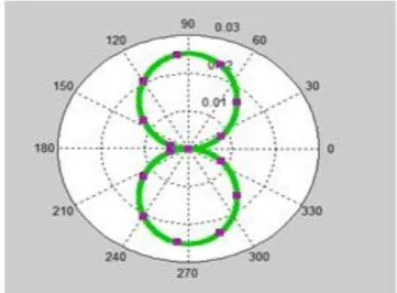
Figure(1) & Figure(3) shows the current waveform of the dipole antenna for length (λ/2) & (λ/10) using the rooftop function, whereas figure(5) & figure(7) shows the current waveform for the respective lengths using pulse function. Figure (2) & figure(4) are the radiation pattern for lengths (λ/2) &(λ/10) using the rooftop function, whereas Figure (6) & figure(8) are the radiation pattern for lengths (λ/2) &(λ/10) using the pulse function.

IV. CONCLUSION

(7)

REFERENCES

1. K. Priyadharshini, Mrs. G. Brenie Sekar ,“Design of Dipole Antenna Using MoM” International Journal of Innovative Research in Computer

and Communication Engineering vol.2. Special Issue 1,pp-1469-1476 March 2014.

2. Tamajit Nag, Dr. Amlan Datta, "Survey on Calculation of Mutual Impedance of Plannar Dipole Array Using Method of Moment", International Journal of Computer Science and Information Technologies, Vol. 6 (1) , 863-865, 2015.

3. Rais Rabani Bin Abd. Rahman, “Analysis Of Non Uniform Surface Current Distribution On Thick And Thin Wire Antenna”, A project report

submitted in partial fulfillment of the requirement for the award of the Degree of Master of Electrical Engineering Faculty of Electrical and Electronics Engineering University Tun Hussein Onn Malaysia pp-7-13 June 2013.

4. Yazdan Mehdipour Attaei, “Current Distribution on Linear Thin Wire Antenna Application of MOM and FMM” Submitted to the Institute of

Graduate Studies and Research In partial fulfillment of the requirements for the Degree of Master of Science in Electrical and Electronic Engineering, pp-1-53 February 2012 .

5. Ramesh Garg, “Analytical and Computational Methods in Electromagnetics”,ARTECH HOUSE, INC.685 Canton Street Norwood, MA 02062

,vol 5, pp-445-448, 469-477, 2008.

6. Walton C. Gibson, “The Method of Moments in Electromagnetics” Chapman & Hall/CRCTaylor & Francis Group ,vol. 4, pp- 33-36, 44-49 2008.

7. I. H¨anninen, M. Taskinen, and J. Sarvas, "Singularity Subtraction Integral Formulae For Surface Integral Equations With Rwg, Rooftop And Hybrid BasisFunctions", Electromagnetics Research, PIER 63, pp-243–278, 2006.

8. Järvenpää, S., M. Taskinen, and P. Ylä-Oijala, “Singularity subtraction technique for high-order polynomial vector basis functions on planar triangles,” IEEE Trans. Antennas Propagat.,No. 1, Vol. 54, pp-42–49, January 2006.

9. C.A. Balanis, “Antenna Theory: Analysis and Design”, John Wiley &Sons, Inc, 3rd edition, pp- 433-440, 443-447, 450-458, 2005.

10. Khayat, M. A. and D. R. Wilton, “Numerical evaluation of singular and near-singular potential integrals,” IEEE Trans Antennas Propagat., Vol. 53, No. 10, pp-3180–3190, October 2005.

11. Robert E. White ,“Computational Mathematics” Published by CRC Press vol. 3, pp-314-321, August 3, 2003.

12. Järvenpää, S., M. Taskinen, and P. Ylä-Oijala, “Singularity extraction technique for integral equation methods with higher order basis functions on plane triangles and tetrahedra,"International Journal for Numerical Methods in Engineering",Vol. 58, pp-1149–1165, 2003.

13. Matthew.N.O.Sadiku,Ph.D .“Numerical Techniques In Electromagnetics”.CRC Press ,Vol 2, pp- 300-316, 2000

14. Tapan K. Sarkar, Antonije R. Djordjevic, Branko M. Kolundzija , “Method of Moments Applied to Antennas” pp-8-10, November 2000.

15. Warren L. Stutzman ,Gary A. Thiele ,“Antenna Theory and Design”, John Wiley & Sons, Inc.vol.2 1998.

16. Smain Amari and Jens Bornemann,"Efficient Numerical Computation of Singular Integrals with Applications to Electromagnetics", IEEE transactions on antennas and propagation, vol. 43, no. 11, november 1995.

17. T.K. Sarkar, “Application of the Conjugate Gradient Method in Electromagnetics and Signal Processing”, pp- 43-56, 1991.

18. Tatsuo Itoh , “Numerical Techniques for Microwave and Millimeter-Wave Passive Structures”. John Wiley &Sons, Inc vol.2, pp-184-192 1991. 19. T.K. Sarkar, K.R. Siarkiewicz, and R.F. Stratton, "Survey of numerical methods for solution of large systems of linear equations for

electromagnetic field problems", vol. AP-29,1981.

20. P. M. ANSELONE, "Singularity Subtraction In The NumericalSolution Of Integral Equations", J. Austral. Math. Soc. (Series B) 22 , PP-408-418, 1981.