Multi-Objective Pathfinding in Dynamic Environments

(1)

University of Windsor University of Windsor

Scholarship at UWindsor

Electronic Theses and Dissertations Theses, Dissertations, and Major Papers

5-7-2018

Multi-Objective Pathfinding in Dynamic Environments

Halen Whiston

University of Windsor

Follow this and additional works at: https://scholar.uwindsor.ca/etd

Recommended Citation Recommended Citation

Whiston, Halen, "Multi-Objective Pathfinding in Dynamic Environments" (2018). Electronic Theses and Dissertations. 7448.

https://scholar.uwindsor.ca/etd/7448

This online database contains the full-text of PhD dissertations and Masters’ theses of University of Windsor students from 1954 forward. These documents are made available for personal study and research purposes only, in accordance with the Canadian Copyright Act and the Creative Commons license—CC BY-NC-ND (Attribution, Non-Commercial, No Derivative Works). Under this license, works must always be attributed to the copyright holder (original author), cannot be used for any commercial purposes, and may not be altered. Any other use would require the permission of the copyright holder. Students may inquire about withdrawing their dissertation and/or thesis from this database. For additional inquiries, please contact the repository administrator via email

(2)

Multi-Objective Pathfinding in Dynamic Environments

By

Halen D. Whiston

A Thesis

Submitted to the Faculty of Graduate Studies through the School of Computer Science in Partial Fulfillment of the Requirements for

the Degree of Master of Science at the University of Windsor

Windsor, Ontario, Canada 2018

(3)

MULTI-OBJECTIVE PATHFINDING IN DYNAMIC ENVIRONMENTS

BY

HALEN D. WHISTON

APPROVED BY:

M. Hlynka

Department of Mathematics and Statistics

A. Jaekel

School of Computer Science

S. Goodwin, Advisor

School of Computer Science

(4)

III

Author

’

s Declaration of Originality

I hereby certify that I am the sole author of this thesis and that no part of this thesis has been

published or submitted for publication.

I certify that, to the best of my knowledge, my thesis does not infringe upon anyone’s

copyright nor violate any proprietary rights and that any ideas, techniques, quotations, or any

other material from the work of other people included in my thesis, published or otherwise, are

fully acknowledged in accordance with the standard referencing practices. Furthermore, to the

extent that I have included copyrighted material that surpasses the bounds of fair dealing within

the meaning of the Canada Copyright Act, I certify that I have obtained a written permission

from the copyright owner(s) to include such material(s) in my thesis and have included copies of

such copyright clearances to my appendix. I declare that this is a true copy of my thesis,

including any final revisions, as approved by my thesis committee and the Graduate Studies

office and that this thesis has not been submitted for a higher degree to any other University or

(5)

IV

Abstract

Traditional pathfinding techniques are known for calculating the shortest path from a given start

point to a designated target point on a directed graph. These techniques, however, are

inapplicable to pathfinding problems where the shortest path may prove to be hazardous for

traversal, or where multiple costs of differing unit-types lie along the same path. Moreover, the

shortest path may not be optimal if it requires forfeiting a valuable resource. While strategic

methods have been proposed in the past to completely avoid paths determined to be dangerous,

these methods lack the functionality to provide agents the ability to decide which resources are

more valuable for conservation, and which resources possess the greatest risk at being lost.

For environments where risk varies dynamically across edges, we propose a solution that can

determine a path of least expected weight based on multiple properties of edges. With this

Multi-Objective Pathfinding technique, agents can make decisions influenced by highest priority

objectives and their preferences to trading off some resources for others. The solution is based on

traditional pathfinding techniques, extending their usability to cover strategic and dynamic

scenarios where additional properties contained within the search map could render them useless.

Nevertheless, our solution is compatible with problems where the goal is to simply find the least

weighted path, otherwise known as the objectively resource-conservative path among a set of

(6)

V

Dedication

To my beloved family:

Grandparents: Theresa (Lain) & Phillip Yoong, Helen & Dennis Whiston.

Parents: Priscilla & Jason.

(7)

VI

Acknowledgements

I would like to thank Dr. Scott Goodwin for working as my advisor and providing guidance

throughout the course of my graduate term at the University of Windsor. I am honoured to have

had this opportunity to work with him and could not have asked for a better supervisor, speaking

as a relatively new member in the field of scientific research.

I would like to thank my internal reader, Dr. Arunita Jaekel, for showing her support and having

an interest in my research area. I would also like to thank my external reader, Dr. Myron Hlynka,

for providing his support for my defense.

I would like to give a special thanks to the graduate secretary, Mrs. Karen Bourdeau, for helping

me whenever I had difficulties understanding the logistics of the program, and also for answering

questions I had pertaining to the curriculum in general. Her assistance was greatly appreciated.

Finally, I would like to thank my family for supporting me over the course of my academic

(8)

VII

List of Figures

Figure 1: Waypoint Navigation ... 3

Figure 2: Navigation Mesh ... 4

Figure 3: Manhattan Distance vs Euclidean Distance ... 7

Figure 4: A* Search ... 13

Figure 5: Extended A* with Survivability Application ... 17

Figure 6: Extended A* with Survivability Work Flow ... 19

Figure 7: Static Single Resource (Problem Graph) ... 29

Figure 8: Static Single Resource (Expanded Search Tree) ... 30

Figure 9: Static Multiple Resources (Problem Graph) ... 32

Figure 10: Static Multiple Resources (Expanded Search Tree) ... 33

Figure 11: Static Single Resource with Expected Values over Independent Events (Problem Graph) ... 35

Figure 12: Static Single Resource with Expected Values over Independent Events (Expanded Search Tree) ... 36

Figure 13: Static Multiple Resources with Expected Values over Independent Events (Problem Graph) ... 38

Figure 14: Static Multiple Resources with Expected Values over Independent Events (Expanded Search Tree) ... 39

Figure 15: Static Single Resource with Expected Values over Dependent Events (Problem Graph) ... 40

Figure 16: Static Single Resource with Expected Values over Dependent Events (Expanded Search Tree) ... 41

Figure 17: Static Multiple Resources with Expected Values over Dependent Events (Problem Graph) ... 42

Figure 18: Static Multiple Resources with Expected Values over Dependent Events (Expanded Search Tree) ... 44

Figure 19: Dynamic Single Resource with Known Termporal Values (Problem Graph) ... 46

(11)

X Figure 22: Dynamic Multiple Resources with Known Temporal Values (Expanded Search Tree)

... 51

Figure 23: Dynamic Single Resource with Expected Values over Independent Events with Known Temporal Values (Problem Graph) ... 53

Figure 24: Dynamic Single Resource with Expected Values over Independent Events with Known Temporal Values (Expanded Search Tree) ... 55

Figure 25: Dynamic Multiple Resources with Expected Values over Independent Events with Known Temporal Values (Problem Graph) ... 56

Figure 26: Dynamic Multiple Resources with Expected Values over Independent Events with Known Temporal Values (Expanded Search Tree) ... 61

Figure 27: Dynamic Single Resource with Expected Values over Dependent Events and Known Temporal Values (Problem Graph) ... 62

Figure 28: Dynamic Single Resource with Expected Values over Dependent Events and Known Temporal Values (Expanded Search Tree) ... 63

Figure 29: Dynamic Multiple Resources with Expected Values over Dependent Events and Known Temporal Values (Problem Graph) ... 64

Figure 30: Dynamic Multiple Resources with Expected Values over Dependent Events and Known Temporal Values (Expanded Search Tree) ... 70

Figure 31: Process Overview ... 62

Figure 32: Pathfinding Framework ... 74

Figure 33: Pathfinding Framework with A* Search Demonstration ... 75

Figure 34: Pathfinding Framework with A* Search Nodes that are Explored ... 77

Figure 35: Obstacle Distribution ... 78

Figure 36: Runtime Analysis - Experiment 1... 86

Figure 37: Final G-Value Comparison - Experiment 1 ... 87

Figure 38: Pathfinding Framework with Dijkstra's Algorithm Demonstration ... 89

Figure 39: Pathfinding Framework with Multi-Objective Pathfinding Demonstration ... 89

(12)

XI

List of Algorithms

Dijkstra’s Algorithm

A* Search

Lifelong Planning A*

Extended A* with Survivability

(13)

1

Chapter 1: Introduction

1.1 Problem Domain

Determining the shortest path from a start position to a destination is a necessary goal for

travelers, as the shortest possible route will always lead to the least amount of resources being

spent. [1] This process is commonly known as pathfinding, and it is widely used within the game

development industry, typically in the form of computer-controlled agents that rely on artificial

intelligence for their path planning in order to provide an engaging experience for the player.

Outside of entertainment software, pathfinding may also see uses in optimizing resource space in

warehouse management and geographical exploration.

Traditionally, pathfinding has been used to determine a minimum cost path between nodes

through the use of several best-first search algorithms that rely on resource-related or

distance-related costs. While this field has been widely studied by numerous contributors in the past, the

situation changes when a probabilistic factor is included in the problem that attributes to

modifications in edge costs. A prime example of this would be in a battlefield setting, where

certain areas on the graph may be treacherous for the agent to traverse due to strategically placed

hazards (landmines, sentries, etc.). If the probability of triggering one of these hazards is too

great, it may be more beneficial for our agent to find an alternative route around these hazards,

even if the optimal path requires the agent to take a risk. Conversely, if the risk of danger is not

great, then perhaps traversing the hazards would lead to an optimal solution after all.

(14)

2 not being able to find the shortest path. It is in cases like these where the shortest distance path

no longer becomes our optimal path, as choosing to follow such a path could forfeit valuable

resources (such as the agent’s vitality in the example). This type of scenario adds another layer to

traditional pathfinding problems in the form of additional properties contained within the search

map.

1.2 Pathfinding

The objective in pathfinding (or path planning) is to find an optimal path that can be routed

between two predetermined nodes, referred to as the start node and the goal node respectively. If

we map this out on a graph G, we can consider two existing vertices on that graph, s and g and

the various paths that may exist between them in order to determine an optimal solution. This is

the type of problem travelers are presented with when they have to find a path from their current

location to their destination. We refer to the travelers utilizing pathfinding strategies as agents.

An agent can be best described as, “a system situated within and a part of an environment that

senses that environment and acts on it, over time, in pursuit of its own agenda and so as to affect

what it senses in the future.” [2] In the simplest of cases, the agent represents the actor or

character utilizing the pathfinding solution in the environment.

1.2.1 Graph Representation

Pathfinding environments are often represented as maps, typically in one of three classic

representations: Grids, Waypoint Graphs, and Navigation Meshes (abbreviated Navmesh).

Grids are made up of a series of tiles representative of terrain and contain the node data for each

(15)

3 implement in typical pathfinding frameworks due to their block-like structure. In a grid, each tile

represents a node in the map, and each node has its own set of edge-costs that must be paid in

order to allow traversal to or from respective neighbouring nodes.

Waypoint graphs (Figure 1) are another method of map representation. They are composed of a

series of nodes placed at different locations in a map to represent positions an agent can either

stay on or pass through. Lines representing the edges conjoin vertices in a waypoint graph and

denote the edges in which traversal is possible. Waypoint graphs have the added benefit of

containing fewer vertices than a grid layout of the same map, making them ideal for representing

the environment of an enclosed area, or an area that is partitioned. The disadvantage, however, is

that as vertices are added to the waypoint graph, the complexity of both rendering and navigating

these vertices increases, which is why these types of layouts tend to be used in environments

where a minimal amount of nodes is expected.

Figure 1: Search map depicting waypoint navigation. An agent may travel along a nearby edge to reach a neighbouring node. [16]

The final type of graph representation known as a navmesh (Figure 2) is effective at representing

a real-world layout in a graph form. Navmeshes are made up of interconnected polygons;

(16)

4 nodes themselves are within each polygon of a navigation mesh, and agents that are situated in

each polygon have free reign of traversal within that polygon without having to travel to a

neighbouring vertex. This makes navmeshes ideal for representing complex or polygonal terrain,

as the meshes can be altered to fit within the desired environment.

In this thesis, grids will be used to represent the search map for all experiments pertaining to the

proposed solution.

Figure 2: Search map depicting navigation using navmeshes. An agent may freely move within an area of a navmesh if a node it is stationed on occupies it. [16]

1.2.2 Search Algorithms

For solving pathfinding problems, search algorithms are used to find an optimal path between

any two vertices on a graph. Uninformed search algorithms such as Depth-First Search and

Breadth-First Search exhaust every possible node relative to the starting position until the goal is

reached. They are a type of brute force approach, as no knowledge of the destination’s location is

kept in memory. Conversely, informed searches can more accurately discern the location of the

goal by utilizing known attributes of edge-weights. Dijkstra’s Algorithm, for example, finds and

(17)

5 only choosing to follow the edges with the smallest weights, the method can effectively route the

shortest path without having to visit nodes that may never need to be traversed. It is more

efficient than typical uninformed searches, since there is a direct correlation between the speed

of a solution and the number of nodes that require expansion, as described by Nilsson et al.

where optimal algorithms “examine the smallest number of nodes necessary to guarantee a

minimum cost selection.”[4]

1.2.3 Admissibility

The goal of pathfinding is to generate a subgraph representative of an optimal path from any

given node s to its respective goal node g. We refer to these algorithms as admissible if they can

guarantee to find an optimal path if such a path exists in the graph. [4] Likewise, when using

heuristics for informed searches, it is imperative that the estimated cost never exceeds that of the

actual cost to reach a respective node. Moreover, consistent heuristics must satisfy the triangle

inequality:

฀ = 0

ℎ ≤ , ’ + ℎ ’ ; ∈ ’ ∈ ℎ ≠ 𝑔 𝑎

Where h(n) represents the heuristic function of the current node, n. The triangle inequality

ensures that the heuristic value will consistently be less than or equal to the actual cost of the

current node to its neighbour plus the estimated distance of the neighbour to the goal, resulting in

equal estimation at worst. It is this property that defines heuristic consistency, meaning that the

sum of two sides of a triangle must be longer than each individual side. The A* Search algorithm

is a prime example of a pathfinding solution that relies on admissible heuristics, as not only is the

(18)

6 never overestimated relative to the actual costs between nodes. Admissible heuristics will always

be optimistic with regards to cost estimation. [1]

In general, the informedness of a heuristic is comparable to other potential heuristics under the

following theorem:

∀ | ℎ ≤ ℎ ≤ ℎ𝑥 → ℎ ℎ ℎ

A heuristic that is more informed than the alternative will also find the optimal path by

expanding fewer nodes in the same scenario.

1.2.4 Heuristics

Informed searches rely on knowing information about the problem domain, and are able to do so

through the use of heuristics. Heuristic functions provide a means of estimation, further reducing

the number of expanded nodes as opposed to uninformed searches. In traditional pathfinding

solutions, estimations typically include calculating a minimum distance from neighbouring nodes

to the goal, which is an objectively more informed method than greedily expanding the closest

neighbour relative to the current position. As such, the subgraph of expanded nodes generated

tends to grow towards the direction of the goal.

Traditionally, two forms of heuristic functions are used to calculate cost estimations:

1. Manhattan Distance

2. Euclidean Distance

The Manhattan Distance is calculated based on the distance between two points along the axes of

grid lines. The term is inspired by the grid-like structure of road networks in Manhattan, New

York. The sum of the grid lines forming the distances between the two points becomes a

(19)

7

ℎ = (| − |) + (| − |)

Where and are points on a grid, and = , and = ( ), respectively.

The Euclidean Distance is somewhat different from the Manhattan Distance (Figure 3), as

instead of the distance being calculated along the lines of the grid, it is calculated as the length of

a straight line formed between two points. The formula can be described as follows using the

Pythagorean Theorem:

h(n) = √( − ) + ( − )

Where, again, and are points on a grid, and = , and = ( , ) respectively.

It should be noted that the approach proposed in this thesis utilizes Euclidean Distance for any

heuristic calculations.

Figure 3: Depiction of Manhattan Distance versus Euclidean Distance. [17]

1.3 Optimal Path

In traditional pathfinding problems, the optimal path between two nodes is always the shortest,

however, depending on the context of the problem the optimal path has different meanings. For

(20)

8

safest path, provided that danger and survival are accounted for in the scenario. [7] We must note

that the optimal solution will not always be the same across similar pathfinding problems,

depending on the context and how we choose to define what our optimal path should be.

1.4 Thesis Contribution

This research has several contributions to the study of pathfinding. First and foremost, have

extrapolated the concept of traditional pathfinding problems to applications where the loss of

multiple resources is to be minimized instead of just one. In essence, we made some

modifications to traditional pathfinding solution approaches in order to solve a specific type of

scenario that would otherwise go unsolved. Additionally, our solution has been developed to

include risks (more specifically, weights that have a probability tied to their values) that may

arise in environments, inspired by the works of other authors and their strategic solutions. These

modifications extend the usability of traditional pathfinding solutions to handle problems they

normally could not handle before. Flexibility in resource prioritization is also included in our

solution, and also ensures compatibility with existing systems due to the nature of the solution

being an extension of traditional pathfinding solutions. Whatever the case, our research aims to

be applicable to all types of environments. Furthermore, with a relationship to previous

algorithms such as A* Search established, we also attempt to identify an accurate heuristic, much

like that which is used in traditional A* Search. An accurate heuristic that can be applied to

Multi-Objective Pathfinding could also potentially lead to additional related solutions in the

future. Finally, this work includes not only an algorithmic solution to the problem but also a

testing bed in the form of a pathfinding framework for comparing and experimenting with

(21)

9

1.5 Thesis Outline

This thesis is divided into seven chapters, the bulk of which will be in Chapter 3. Chapter 1

covers the introduction to pathfinding and familiarizes the reader with concepts typically seen in

research related to pathfinding. In Chapter 2, we will be analyzing various other methods used in

pathfinding, including their uses, advantages, drawbacks, and applications. Chapter 3 will cover

our proposed approach to Multi-Objective Pathfinding, and will also discuss several scenarios to

the theory behind its intended applications. A total of twelve scenarios will be covered, each one

building upon the previous before a general solution to cover all cases will be presented. In

Chapter 4, we describe our experimental setup, limitations, assumptions, and system structure

related to any experiments. Chapter 5 will show the results of our experiments and comparisons

between our approach and existing solutions, including Dijkstra's Algorithm and A* Search.

Chapter 6 marks our concluding remarks on the subject material, and Chapter 7 provides an

(22)

10

Chapter 2: Background

In this section, we review various types of pathfinding algorithms and their uses in the field.

While the work presented in this document is related, the basis of the solution borrows from

approaches that have previously proven to be successful. Traditionally, the goal of pathfinding

has been to find the least weighted path through a series of interconnected vertices, and many of

the algorithms that will be mentioned here are based on this principle. For the purposes of this

section and all other areas mentioned within this document, the notion of a traditional

pathfinding algorithm is used to describe solutions that can be applied to the classical problem of

searching a graph for the shortest possible path between two vertices.

2.1 Dijkstra

’

s Algorithm

The idea behind a best-first search algorithm is as follows: Given a set of vertices on a graph and

the traversal cost of each node relative to our starting position, we choose to explore the nodes

whose cost is the minimum and expand its children from there. [14] Comparisons can be made

between the current path and potentially shorter paths in order to find a true optimal path. By

only choosing to follow the edges we estimate to be the least expensive, we can eventually

obtain the shortest path. By doing so, we derive a greedy solution that also guarantees an optimal

path (assuming there is at least one possible path toward the goal in the first place). Dijkstra’s

Algorithm is such an example of best-first search algorithms, which is based on the concept of

navigating directed graphs while minimizing the “distance travelled” at the same time. The

problem is determining a path in which the number of resources spent can be minimized, as

(23)

11 work. If the distance traversed can be minimized, then naturally the amount of time and

resources spent reaching a given destination will also be minimal. Dijkstra uses the idea that each

node in a graph can be broken down into different sets in order to define their states as the

following:

1. Visited

2. Next to be visited

3. Not yet visited

The starting node becomes the initial visited node in the set and from there the algorithm

branches out to neighboring nodes, comparing multiple paths from the current node and choosing

the shortest path between them. From the paths extending the newly visited paths, the next

smallest path to the neighbouring nodes can be determined, accumulating from the weight of the

paths previously traversed. Following this idea of only choosing the shortest paths based on the

current node being visited, the minimal path branching from the origin node to every other node

(24)

12 Algorithm 1: Dijkstra’s Algorithm Pseudo-code

Input: Node start, Node goal

1: Main()

2: openList := ∅; //priority queue based on g 3: closedList := ∅;

4: g(start) := 0;

5: openList.Insert(start); 6: while openList != ∅ do

7: current: = openList.Pop(); 8: if current == goal then 9: return 'path found';

10: closedList.Insert(current); 11:

12: for each neighbour Є current.Neighbours do 13: if neighbour in closedList then

14: continue;

15: if not neighbour in open then 16: openList.Insert(neighbour);

17: if g(current)+ c(current,neighbour) < g(neighbour) then 18: g(neighbour) := g(current) + c(current, neighbour); 19: parent(neighbour) := current;

20: return 'path not found'; 21: end;

2.2 A* Search

Using Dijkstra’s Algorithm as a base, the A* Search algorithm attempts to obtain a more

informed search as opposed to greedily choosing the nearest neighbour without any knowledge

of where the goal is located. In order for this algorithm to function, all nodes in the graph are

required to track their own secondary cost that represents the estimated distance relative to the

goal position. Each node is aware of both its cost of traversal from the starting node and its

estimated distance from the goal. Using these key values (denoted by a g(x) and h(x) function

respectively), a more informed search than that of Dijkstra’s Algorithm can take place and will

(25)

13

Figure 4: Evaluated path using A* Search [18].

At a high level, A* Search can be used to find the shortest path within a directed graph from a

starting point s and an ending point g. The algorithm uses the knowledge based on the

surrounding nodes from the current point and calculates the shortest possible route to the next

node, while also taking into consideration the actual distance from the current node to the

destination node [15]. The function is described as:

= + ℎ

where g(n) calculates the distance from the current node to the next node, and h(n) calculates the

estimated distance from the current node to the destination node. The minimum distance returned

from this function over a series of nodes is the minimized route and thus the shortest path. It

follows a breadth-first search ideology, analyzing the open list, which is a list of available points

to traverse from the current node. The g(n) value is calculated as the cost to go from one node to

the next, whereas the h(n) value represents the heuristic or the actual distance from a given node

(26)

14 the next node to recalculate g(n) for and the cycle continues until the goal node is reached, at

which point a path can be drawn from the goal back to the starting node [15].

Algorithm 2: A* Search Pseudo-code

Input: Node start, Node goal

1: Main()

2: openList := ∅; //priority queue based on f 3: closedList := ∅;

4: g(start) := 0;

5: f(start) := g(start) + h(start); 6: openList.Insert(start);

7: while openList != ∅ do

13: for each neighbour Є current.Neighbours do 14: if neighbour in closedList then

15: continue;

16: if not neighbour in open then 17: openList.Insert(neighbour);

18: if g(current)+ c(current,neighbour) < g(neighbour) then 19: g(neighbour) := g(current) + c(current, neighbour); 20: f(neighbour) := g(neighbour) + h(neighbour);

21: parent(neighbour) := current; 22: return 'path not found';

23:end;

Two lists are maintained during processing, appropriately labelled the open and closed lists in

typical implementations. Upon initialization, the starting node is added to the open list and is

subsequently “expanded” in order for successor nodes to be realized. These successors are then

added to the open list, while the predecessor enters the closed list (or alternatively is labelled as

visited). From here, the f-scores of successors are compared to the predecessor, and the minimum

(27)

15 the open list have been exhausted, or the designated goal node has been expanded. The final

procedure involves tracing the path all the way back from the goal node to the start node, using

each node’s predecessor to denote the path.

Similarly to Dijkstra’s Algorithm, A* Search need only rely on two properties that exist within

the nodes, which can be used to represent a geographical map realistically. In a realistic setting,

however, this information may not lead to a preferred path if danger should lie within the optimal

path itself. In this way, it suffers from the same drawbacks as Dijkstra’s Algorithm in that this

solution will find the absolute shortest path regardless of how dangerous or unpreferred a path

may be. It will surely find a solution within a reasonable time, but it’s applications to a problem

beyond the scope of the shortest pathfinding problem are somewhat limited. That being said, A*

Search is one of the most commonly used pathfinding algorithms in the industry and has been

easily replicated in pathfinding solutions and video game entertainment software.

2.3 Lifelong Planning A*

The majority of the solutions mentioned in this thesis are of the heuristic or uniformed types,

meaning that they either rely on a heuristic for estimated closest paths, or they cascade through

the nearest neighbours as in Depth-First Searches or Breadth-First Searches. The works of

Koenig et al. propose Lifelong Planning A*, which is an incremental solution inspired by the A*

Search approach, which utilizes a heuristic. The incremental nature of the algorithm lends itself

to be similar to A* Search on its first iteration. However, subsequent iterations are capable of

finding alternate paths in an environment where small changes occur near the optimal route. [8]

This is because the solution “reuses information from previous searches,” essentially reducing

(28)

16 ignoring any recomputation required to those specific cells. A secondary value in addition to the

primary cost value of each node is maintained, known as the rhs-value which is derived from a

DynamicSWSF-FP algorithm. These rhs-values are one-step lookahead values that track the

minimum cost over all neighbours of the current node traversing over to the next neighbour, and

are thus “potentially better informed than the g-values.” By ensuring that the nodes are locally

consistent (in other words, the g-value of each node equals its respective rhs-value), there is no

need to check node costs relative to the starting node if a change in the environment is made. If a

node’s rhs-value is not equal to its respective g-value, then an inconsistency in the graph has

occurred in one of the current node’s neighbours. These nodes that are locally inconsistent

therefore become the first nodes to be replanned, which ultimately remain a fraction of the total

population of nodes provided only a few edges or vertices were altered in the search map. In the

average case, it is concluded that Lifelong Planning A* can be more efficient than A* Search and

similar A* Search refinement solutions when “the path-planning problems change only slightly,

and the changes are close to the goal.”

2.4 Extended A* with Survivability

Kim et al. introduce an enhanced version of A* Search that attempts to solve the problem of

finding a shortest, safest path in a known environment. As the name implies, the approach is

based on the traditional A* Search algorithm, in that it utilizes costs on the map to evaluate the

shortest path from a given starting point to a specified destination. [13] They provide a real-life

example of an automated combat vehicle that can navigate terrain in a dangerous environment,

typically a war-torn battlefield or similar area where some zone could be treacherous. Since the

(29)

17 is appended to the existing function. They devise a Probability Hit function used to determine

the likeliness of being targeted by an enemy or the chances of encountering a dangerous threat at

any given node. The Probability Hit function represents an added weight onto the cost function

of A* Search, where a survivability rate is included for when nodes are being expanded. Hence,

this algorithm is considered an “extended” version of A* Search because it determines not only

the shortest route but also the safest route based on the likeliness of survivability. [13]

Additionally, an agent could very well traverse through a dangerous node if that same node just

so happens to be on the shortest path to the destination. At a high level, the algorithm can

effectively minimize not only the distance travelled but also the risk of being threatened. It

should be noted, however, that, like its predecessor, the Extended A* Search with Survivability

approach does not handle dynamic environments, and is much better suited to situations where

the risk in an area can be predictable or simply evaluated. It also does not cover situations in

which the agent may wish to prioritize speed over safety, thereby taking a risk in itself in order to

reach its goal within a quicker time frame.

Consider the following example, where our agent represents a soldier and the map

(30)

18

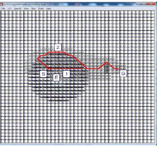
Figure 5: Study of New Path Planning Algorithm Using Extended A* Algorithm with Survivability.

In the demonstration, a soldier may wish to reach their destination in the middle of the

battlefield, but using a regular A* Search would force them to traverse unsafe terrain, which is

represented by the gray circular area on the map. A* would yield path 1 as labelled in the graph.

Following such a path requires heavy traversal through risky terrain, and thus becomes

hazardous to the agent using the algorithm. Imagining that the circular area could represent a

minefield, it would make sense for the agent to reach their destination in the shortest amount of

time possible while also minimizing the risk of being in such an area at any given point in time.

Thus, the Extended A* with Survivability algorithm reroutes the path, giving us the example as

shown in path 2. This path intentionally avoids hazardous areas, navigating on the very outskirts

of the danger zone to find the closest node to the goal. With no other option but to advance

further, the algorithm draws a straight line to the goal from the outskirts of the hazardous area,

(31)

19 situation where risk minimization is to be prioritized over the time it takes to reach the

destination itself, a traditional A* Search approach would not be sufficient.

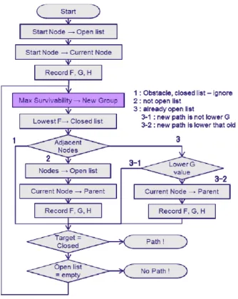
Figure 6: Workflow of Extended A* with Survivability solution. Determining max survivability takes place before the A* Search algorithm is executed.

The drawback to this algorithm is that it will always prioritize safety over minimizing the

distance travelled, and other solutions that rely on maintaining safety over distance also suffer

(32)

20 along the danger zone until it finds that singular node is leading to a path of safety. This becomes

more of a problem when the destination is not that far relative to an agent’s position but is

perceived to be far if the hazardous area encompasses a large portion of the map. Hazardous

areas are essentially treated as obstacles that the agent must either outright avoid or travel close

to in order to reach their designated goal. In a realistic scenario, this type of solution may not be

feasible because, by the time the agent does make it to their goal, they could have tremendously

saved time by simply cutting across the hazardous area and taking a risk as if it were a traditional

pathfinding problem.

2.5 Strategic Pathfinding

Singh and Holder’s work presents a solution to the problem of pathfinding related to a

measurable risk versus navigation time. Their goal was to have the agent navigate an

environment without predetermined waypoints and strategically make decisions based on the

estimated likelihood of encountering an enemy, which they depicted in a combat simulator.

Calculations pertaining to the probability of being struck by an attack at each point in the map

also factors into the pathfinding strategy. This provides more flexibility in the pathfinding

decision-making that previously mentioned solutions do not cover. Unlike these methods that

prioritize one resource over another, the Strategic Pathfinding method accounts for risk, in

addition to the time it would take for an agent to reach its goal. A strategic path is defined to be,

“a trade-off between the time of traversal and the risk along the path.” [7]

Two levels of abstraction are required to utilize a strategic pathfinding method. The Area level

defines a set of areas that an agent may walk over, and is abstracted from the search map in order

(33)

21 represents the set of actual traversable points that can be navigated through across each area.

Having multiple levels plays into the movement options of the agent, such as knowing when to

walk, jump, or sprint, which can affect the time of traversal in certain areas. The risks themselves

are determined from the Meta-Weight function, a cost that is a modification of the standard edge

costs used by traditional pathfinding algorithms. This Meta-Weight, while coinciding with the

presence of potential risks in an area, alter the paths of agents that otherwise would go

unaffected. The risk itself is calculated based on a function specific to their testbed, essentially

representing the hit probability of being struck by an enemy at a specific node or area. More

detail will be given on this in later sections, as the hit probability essentially represents the risk,

which is the factor that will be affecting our approach to strategic pathfinding. Technically

speaking, the risk can be attributed to the probability of losing a valuable resource, whether that

resource is the vitality of the agent or some other property that holds just as much value

depending on the scenario. The hit probability (or probability of resource loss) can be

represented as a percentage of danger distributed over each area, and may be calculated as given:

𝐻 𝑎 = 𝐻 + 𝐻 − 𝐻 + ⋯ + 𝐻 − 𝐻 − − 𝐻 − … − 𝐻

where HPtotal represents the probability of danger along a given path.

In short, risk along the length of a path can be determined by calculating the total risk with each

node in sequence, multiplied by the chances of not being in danger within each node previously

passed. The result becomes a total amount of risk that can be associated with a path, or any

specific node along that path. Nevertheless, by having an accurate representation of how much

risk is in an area, the path processing can choose to allow the agent to avoid such hazardous

(34)

22 itself. Naturally, this preference is determinable by the type of implementation at hand, and can

make the difference between an agent that will run through a zone of enemy fire, or taking the

safer way out by fleeing instead. Choosing to follow a safer route will result in having to expand

more nodes compared to shorter routes if the hazardous nodes just so happen to be blocking the

otherwise shortest path.

Algorithm 3: Strategic Pathfinding Pseudo-code

Input: Node start, Node goal, Float p

1: Main()

2: openList := ∅; //priority queue based on g 3: closedList := ∅;

4: g(start) := 0;

5: openList.Insert(start); 6: while openList != ∅ do

12: for each neighbour Є current.Neighbours do

13: if neighbour in closedList then 14: continue;

15: if not neighbour in open then 16: openList.Insert(neighbour); 17: risk := CalcRisk(current);

18: if g(current)+ c(current,neighbour) * (risk * p + 1) < g(neighbour) then

19: g(neighbour) := g(current) + c(current, neighbour); 20: parent(neighbour) := current;

21: return 'path not found'; 22:end;

23:CalcRisk(c) 24: current := c;

25: risk := risk(current);

26: while parent(current) != null do

27: risk := risk * (1-risk(parent(current))); 28:

(35)

23

32: return risk + CalcRisk(parent(current)); 33:end;

For evaluating risk over a path, Singh and Holder utilize the Meta-Weight formula, which is a

function that represents edge costs as a factor of weight, risk, and the agent’s preference. [7]

They describe this function as follows:

ℎ = 𝐻 ∗ 𝑅 𝑇 + ∗

Where HP designates the hit probability, and RiskVsTime designates the preference factor of the

agent. In this case, the hit probability can be equated to the probability of forfeiting a resource

(or risk). As for RiskVsTime, this variable can be any value greater than 0, as the higher the

value, the more intensely the agent will pursue a safer path. By referring to a safer path, we are

referring to the path that yields the least amount of risk. In either case, one resource is planned to

be minimized along the subgraph, which is done through the use of Dijkstra's Algorithm after

some cost manipulation with the preference factor and risk. The urgency of objectives may be

calculated separately from the actual pathfinding, and from this, it can be determined how

important certain objectives may be to the agent relative to the specific resource (typically risk

versus distance) to be minimized along a perceived path.

This ability to minimize costs while also providing some form of strategy has been utilized in

studies before. [10] Drawbacks of this solution typically imply a specific type of map setup for it

to be usable, thus making it impractical for broad applications. Furthermore, the Strategic

Pathfinding method comes with the disadvantage of weights being required to be within a certain

threshold for the preference factor to have a large enough bearing on the pathfinding process.

(36)

24 skewing the results. In the following section, we will look at ways to mitigate this disadvantage,

as well as a means to generalize the cost function so that strategic methods can be more

(37)

25

Chapter 3: Proposed Approach

3.1 Motivation

Path planning research has typically been derived from the notion of attempting to find the

shortest existing path in a limited search space. In all cases, the path of least cost will always

yield the most efficient traversal time, but realistically this path may not be the most feasible

depending on the resources that are at stake. For example, an auto-piloted supply truck would not

want to follow the shortest path to its destination if such a path required it to travel through a

minefield, else risking the possibility of losing supplies or the vehicle itself. Similarly,

commuters who frequently crossroads on their way to work may find themselves with the

dilemma of crossing the road prematurely or heading to the crosswalk where travel would be

safer for pedestrians. Logically, the crosswalk is the safest point at which to start crossing from,

but if a commuter should be behind schedule, then they are more likely to act impulsively in

order to reach their destination on time. Thus, taking the risk would be more beneficial by saving

travel time. At what point, however, would it be optimal for a person to cross the road

prematurely as opposed to waiting patiently for the hazards to clear? The solution can be

described as a tradeoff between two resources (in this case, the distance to be covered and the

person’s own vitality), both of which the agent may wish to minimize, but can only prioritize one

over the other, or potentially a little bit of both. This question became the basis for

(38)

26

3.2 Notation

In graph theory, a graph defined G is a set {vi} of vertices (nodes) and a set {eij} of

interconnected edges (arcs) (see Nilsson et al.). Any edge epq that exists on the graph implies a

connection between vertices vp and vq, and vq is a successor of vp. [4] Let V = {vi} as a set of

vertices, and E = {ej} as a set of edges. Each edge has with it an associated weight (or cost) that

is defined as W = {we}, where e denotes the current edge. We can broadly define a directed

weighted graphG = (V, E) where:

= { 1, 2, 3, . . . , |𝑉|} is the set of vertices,

= { 1, 2, 3, . . . , |𝐸|} is the set of edges,

= { 1, 2, 3, . . . , |𝐸|} is the set of edge-weights.

Each edge is an ordered pair ( , ) which denotes the existence of a directed edge from vertex

to vertex . The number of vertices in the graph is | |, the number of edges in the graph is

If there is an edge from vertex to vertex , is said to be adjacent to . Adjacencies in a

list. A path is a sequence of connected vertices , ₊₁, . . . , (or, equivalently, a sequence of

edges , ₊₁, ₊₂, . . . , ₋₁_, ). The weight of a path is the sum of the weights of the edges of

the path.

A comparison can be made to traditional graphs in pathfinding problems, where an edge only

has one resource type associated with it (such as distance). In pathfinding, the vertices of the

(39)

27 locations. Weights typically represent distances, and the objective is to find the shortest (least

weighted) pathway through the graph from a starting vertex to a goal vertex _𝑔.

In this chapter, we will describe several instances of the multi-objective pathfinding problem

through the use of scenarios. Each scenario depicts an example of a very simple search map (for

ease of explanation) and how its properties require different solutions for processing the data.

Specific keywords are used to define each scenario individually and outline the various

differences between them. There are six keywords in total, which are defined as follows:

 Single (Resource): Each edge in the graph contains one value that makes up the total

weight. This is the attribute that traditional pathfinding solutions work with.

 Multiple (Resource): Each edge in the graph contains at least two values that make up the

total weight.

 Deterministic: Costs do not utilize random variables in their calculations.

 Stochastic: Costs utilize random variables in their calculations, and so expected values of

events must be evaluated. Stochastic scenarios come with two subclasses:

o Independent: The result of future events does not rely on previous events.

o Dependent: The result of future events relies on previous events.

 Static: Properties of the graph do not change over the course of the pathfinding process,

such as in traditional pathfinding problems.

 Dynamic: Properties of the graph will change over the course of the pathfinding process.

(40)

28 Scenario

Single/Multiple Deterministic/Stochastic-Independent/Stochastic-Dependent

Static/Dynamic

1 Single Deterministic Static

2 Multiple Deterministic Static

3 Single Stochastic-Independent Static

4 Multiple Stochastic-Independent Static

5 Single Stochastic-Dependent Static

6 Multiple Stochastic-Dependent Static

7 Single Deterministic Dynamic

8 Multiple Deterministic Dynamic

9 10 11 12 Single Multiple Single Multiple Stochastic-Independent Stochastic-Independent Stochastic-Dependent Stochastic-Dependent Dynamic Dynamic Dynamic Dynamic

3.2.1 Scenario 1: Static Single Resource

Applications for Scenario 1 include those commonly seen in traditional pathfinding problems

and are exemplified by Dijkstra’s Algorithm and A* Search. A single resource (typically

representing the remaining distance an agent has to travel between each node) is situated on each

edge and is a cost to be minimized. Characters in a game environment that are only concerned

with minimizing the distance of travel can greatly benefit from this solution, hence why this

(41)

29

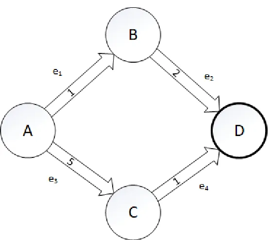
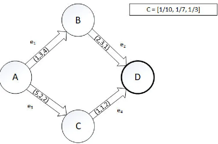
Figure 7: Problem Graph featuring a static single resource per edge.

We define our sets like so:

= { , , , }

= { 1, 2, 3, 4}

= { 𝑒1, 𝑒2, 𝑒3, 𝑒4} = { , , , }

(42)

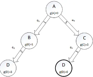
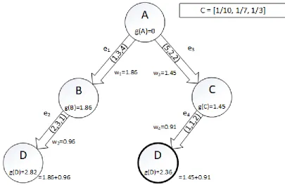
30

Figure 8: Expanded search tree featuring a static single resource using the aforementioned Problem Graph (Figure 7). Two paths are realized with one path yielding less cost than the other.

In multi-objective pathfinding, the weights represent a combination of values of multiple

resources. For example, an edge weight might be used to represent a combination of the distance

travelled and fuel consumption. The objective is to find a path of least cost where weight is

defined as a function of the resources.

The resources in multi-objective pathfinding can be expressed as a × | | matrix R where there

is a row for each resource and a column for each edge. 𝑅[ , ] represents the amount of resource i

expended when traversing edge j. To determine the weight of an edge in a multi-objective graph,

a 1× conversion vector = { ₁, ₂, . . . , } is defined, where each conversion factor represents

the value of the associated resource in terms of some standard units. For example, if we could

travel a longer path, yet save fuel, the conversion factor between distance and fuel would be

based on how much extra distance we would be willing to travel to save a given amount of fuel.

(43)

31 algorithm in that it measures the intensity of a particular resource relative to another as opposed

to the intensity of wanting to take a risk. Moreover, this value converts the units of the resource,

normalizing the formula so that like terms can be collected.

Under this scheme, = 𝑅. Using the conversion vector to convert the resource matrix to

the edge-weight vector provides the ability to solve multi-objective pathfinding problems using

the same A* framework utilized in shortest path problems.

3.2.2 Scenario 2: Static Multiple Resources

While A* Search remains to be one of the most commonly used solutions in the industry, it is not

without its drawbacks. The ability to deduce the path of least cost may not be best suited in some

scenarios. If, for example, an agent wishes to travel the shortest amount of distance to reach its

destination, the environment could contain hazards, making some nodes dangerous to cross. In

the most extreme cases, nodes that are hazardous can be treated as obstacles to be avoided. There

is, however, an alternative in the form of appending multiple costs to the same edge and giving

(44)

32

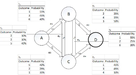
Figure 9: Problem Graph featuring multiple resources. Notice that each edge contains multiple values to denote weight.

Given the above example, we define our sets like so:

= { , , , }

= { 1, 2, 3, 4}

= { 1 , 2 , 3 , 4 }

𝑅 = [ ]

= [ , , ]

Now, by using the formula = 𝑅:

= {[ ∗ + ∗ + ∗ ] , [ ∗ + ∗ + ∗ ] , [ ∗ + ∗ + ∗ ] , [ ∗ + ∗ + ∗ ]}

Implying:

(45)

33

≈ { . , . , . , . }

The expanded search tree used by A* is illustrated as such:

Figure 10: Expanded search tree featuring multiple resources using the aforementioned Problem Graph (Figure 9). Two paths are realized with one path yielding less cost than the other.

Applications of this solution are found in situations where an agent has to pay multiple costs in

order to traverse an edge. Say, for example, a car has to pass over different types of terrain such

as dirt, sand, and ice and each of these terrain types litter the search map in patches. Driving over

sand causes more rotations of the tires than dirt, and even more for driving over ice. The distance

to the destination will remain the same, but resources such as fuel are also added as costs for

each terrain type. Thus, a decision must be made on whether the distance to minimize should

take priority over the usage of fuel, and the conversion rate must be modified to accommodate

(46)

34 Edges may also contain risks, which act as further alterations to existing resource costs. With

risks involved, resources no longer have a set flat cost, but a series of possible costs each with

their own probabilities of occurrence. In other words, each resource becomes an event, with an

expected value that can be calculated using a familiar formula.

We can derive an expected value of a random variable , denoted ’ , using the following

function inspired by the notation cited by R. Hamming:

’ = ∑ ∗

Where is the probability of an event i, and is a discrete random variable representing a

single outcome of event i. [3] Let be a discrete random variable with a set of possible

outcomes 𝛺. Let be one element of 𝛺 and be the probability of the outcome being (i.e.

= = ). Using a six-sided die example, each side of the die is given a value from 1 to 6.

The possible outcomes of are the elements of set 𝛺:

∈𝛺 = { , , , , , }

Applying the formula to this problem knowing that the odds of rolling any one particular side are

⅙, the outcome versus probability distribution can be described in the following table:

Outcome Probability

1

2

3

4

(47)

35 6

And the expected value can be calculated like so:

’ = + + + + + = .

Given a resource , an event e can be associated to it containing a set of outcomes and

probabilities. The expected value taken from this event becomes the updated value of the

resource. We can extend the resource matrix of the above scenario to include risks.

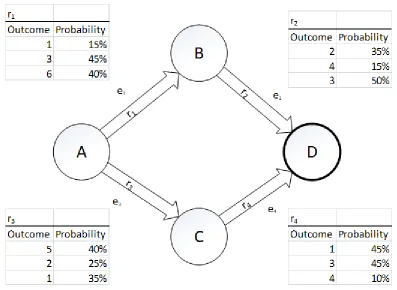
3.2.3 Scenario 3: Static Single Resource with Expected Values over Independent

Events

(48)

36 Resources are now composed of an event, and each event contains a series of pairs (or tuples)

representing an outcome and an associated probability. The notation used for events can be

described as:

𝑥 = { 𝑥 , 𝑥 , … , 𝑥 }

Thus, the expected value of the resources using the R matrix becomes:

’ 𝑅 =[ + + + + + + + + ]

=[ ∗ . + ∗ . + ∗ . ∗ . + ∗ . + ∗ . ∗ . + ∗ . + ∗ . ∗ . + ∗ . + ∗ . ]

’ 𝑅 = [ . . . . ]

Implying:

= [ . ], ₂ = [ . ], ₃ = [ . ], ₄ = [ . ]

≈ { . , . , . , . }

(49)

37 Applications of this solution may be used in situations where there is some uncertainty in the

costs, such as the examples used in Strategic Pathfinding [7]. In Strategic Pathfinding, agents

attempt to reach their designated goal while also reducing their chances of being executed by

hazards along the path. These hazards come in the form of risks, which overall have an effect on

the edge-costs between nodes. It’s ideal that agents will try to travel the path of least cost in

terms of both distance and risk, thus making this solution applicable to that kind of problems.

3.2.4 Scenario 4: Static Multiple Resources with Expected Values over

Independent Events

For scenarios that utilize expected values, it is assumed there is no dependence between the

probability distribution of resources. For example, if the probability distribution changes in one

resource, it does not affect the probability distribution of another resource on the same edge. This

assumption is more applicable to scenarios with known temporal values. However, it should also

be noted for the static cases. Developing a solution that supports joint probability distribution

(50)

38

Figure 13: Problem Graph featuring multiple resources with expected values. Each outcome comes with a probability of occurrence, and thus an expected value can be determined for each resource.

The expected value of the resources using the R matrix becomes:

’ 𝑅

=[ ∗ . + ∗ . + ∗ .∗ . + ∗ . + ∗ . ∗ . + ∗ . + ∗ .∗ . + ∗ . + ∗ . ∗ . + ∗ . + ∗ .∗ . + ∗ . + ∗ . ∗ . + ∗ . + ∗ .∗ . + ∗ . + ∗ .

∗ . + ∗ . + ∗ . ∗ . + ∗ . + ∗ . ∗ . + ∗ . + ∗ . ∗ . + ∗ . + ∗ . ]

’ 𝑅 = [ .. .. .. ..

. . . ]

= [ , , ]

Now, by using the formula = 1 𝑅 :

= {[ ∗ . + ∗ . + ∗ . ] , [ ∗ . + ∗ . + ∗ . ] , [ ∗ . + ∗ . + ∗ ] , [ . + ∗ . + ∗ . ] }

(51)

39

= [ . + . + . ], ₂ = [ . + . + . ], ₃ = [ . + . + ],

4 = [ . + . + . ]

≈ { . , . , . , . }

Figure 14: Expanded search tree featuring multiple resources with expected values using the aforementioned Problem Graph (Figure 13). Two possible paths are realized with one path yielding less cost than the other.

3.2.5 Scenario 5: Static Single Resource with Expected Values over Dependent

Events

In some scenarios, risks may be denoted as part of dependent events, meaning that the

probability of future events occurring changes with each successive outcome in the previous

(52)

40

’ = ∑ ∗ [∏( − ) −

=

] ∗

Where Pi is represented as the probability of the only event occurring and previous events j

failing to occur.

Figure 15: Problem Graph featuring a single resource per edge with expected values.

The expected value of the resources using the R matrix becomes:

’ 𝑅 = [ ∗ . ∗ . − . ∗ . ∗ . − . ]

Implying:

= [ . ], ₂ = [ . − . ], ₃ = [ . ], ₄ = [ . − . ]

≈ { . , . , . , . }

(53)

41

Figure 16: Expanded search tree featuring a single resource with expected values over dependent events using the aforementioned Problem Graph (Figure 15).

3.2.6 Scenario 6: Static Multiple Resources with Expected Values over Dependent

Events

Recall that for Scenario 3, the formula E’ =∑ ∗ , is used for determining the expected

values of costs with independent events. With dependent events, however, we must use the

modified formula as demonstrated in Scenario 4, as the success of subsequent events depends on

(54)

42

Figure 17: Problem Graph featuring multiple resources with expected values. Each outcome comes with a probability of occurrence, and thus an expected value can be determined for each resource. For successive outcomes, the probability of

previous edge-weights needs to be taken into consideration, hence the dependencies.

The example depicted in Figure 13 can be reused in this scenario (see Figure 17), and we can

denote the expected values using the R matrix as follows:

’ 𝑅 = [ ]

Where:

Row 1:

= ∗ . + ∗ . + ∗ . ,

= ∗ . ∗ − . + ∗ . ∗ − . + ∗ . ∗ − . ,

= ∗ . + ∗ . + ∗ . ,

= ∗ . ∗ − . + ∗ . ∗ − . + ∗ . ∗ − . ,

(55)

43

= ∗ . + ∗ . + ∗ . ,

= ∗ . ∗ − . + ∗ . ∗ − . + ∗ . ∗ − . ,

= ∗ . + ∗ . + ∗ . ,

= ∗ . ∗ − . + ∗ . ∗ − . + ∗ . ∗ − . ,

Row 3:

= ∗ . + ∗ . + ∗ . ,

= ∗ . ∗ − . + ∗ . ∗ − . + ∗ . ∗ − . ,

= ∗ . + ∗ . + ∗ . ,

= ∗ . ∗ − . + ∗ . ∗ − . + ∗ . ∗ − .

Thus:

’ 𝑅 = [ .. .. .. ..

. . . ]

= [ , , ]

Now, by using the formula = ’ 𝑅 :

= {[ ∗ . + ∗ . + ∗ . ] , [ ∗ . + ∗ . + ∗ . ] , [ ∗ . + ∗ . + ∗ ] , [ . + ∗ . + ∗ . ] }

Implying:

= [ . + . + . ], ₂ = [ . + . + . ], ₃ = [ . + . + ],

4 = [ . + . + . ]

≈ { . , . , . , . }

(56)

44

Figure 18: Expanded search tree featuring multiple resources with expected values over dependent events using the aforementioned Problem Graph (Figure 17).

3.2.7 Scenario 7: Dynamic Single Resource with Known Temporal Values

In the previous scenarios, maps were described as static, meaning that the properties of the graph

do not change over the course of the pathfinding process. For scenarios 7 and 8, we prepare a

solution catered to edge-weights that may change during processing, and whose values are a

predetermined function of time. We refer to these values as known temporal values. It should be

noted that they may not always evaluate to the same result at any given point during the

pathfinding process.

A new variable t is introduced, representing the current step in time. An extended weight

function that accounts for time is defined as:

(57)

45 Where, similar to Scenario 1, Scenario 3 and Scenario 5, R is a one-dimensional matrix of the set

containing the resources on each edge. During path processing, the value of a resource in R is

calculated for its value at time t. Unlike previous scenarios, however, which do not impose

changes onto the A* Search algorithm itself, one small modification to the cost formula in A*

Search must be made for the dynamic cases:

= ,

Where the total cost leading up to node n accepts the current cost and the current step in time as

parameters. The total cost can now vary depending on the value of t when node n is expanded.

This change is necessary and is stored in each node at the time it is expanded much like in the

previously described A* Search algorithm. This modification to the cost function also holds true

for all remaining scenarios following this point.

The changes may be applied to the existing Dijkstra’s Algorithm on the following lines:

17: if g(current)+ c(current,neighbour,t) < g(neighbour) then 18: g(neighbour) := g(current) + c(current, neighbour,t);

It should be noted that while it is possible for finite loops to occur during the path planning

process, the solution is still guaranteed to find an optimal path so long as one exists. This is not

exclusive to dynamic cases, but static cases as well. Although alternative paths may result in

looping during processing, when the g-value of a dead-end path that is also an alternative

exceeds that of the optimal path, planning will still follow the optimal path as is true for

Multi-Objective Pathfinding in Dynamic Environments

Scholarship at UWindsor

Scholarship at UWindsor

Multi-Objective Pathfinding in Dynamic Environments

Multi-Objective Pathfinding in Dynamic Environments

Multi-Objective Pathfinding in Dynamic Environments

By

Halen D. Whiston

MULTI-OBJECTIVE PATHFINDING IN DYNAMIC ENVIRONMENTS

BY

HALEN D. WHISTON

APPROVED BY:

M. Hlynka

Department of Mathematics and Statistics

A. Jaekel

School of Computer Science

S. Goodwin, Advisor

School of Computer Science

Author

’

s Declaration of Originality

Abstract

Dedication

Acknowledgements

Table of Contents

List of Figures

List of Algorithms

Chapter 1: Introduction

1.1 Problem Domain

1.2 Pathfinding

1.2.1 Graph Representation

1.2.2 Search Algorithms

1.2.3 Admissibility

1.2.4 Heuristics

1.3 Optimal Path

1.4 Thesis Contribution

1.5 Thesis Outline

Chapter 2: Background

2.1 Dijkstra

’

s Algorithm

2.2 A* Search

2.3 Lifelong Planning A*

2.4 Extended A* with Survivability

2.5 Strategic Pathfinding

Chapter 3: Proposed Approach

3.1 Motivation

3.2 Notation

3.2.1 Scenario 1: Static Single Resource

3.2.2 Scenario 2: Static Multiple Resources

3.2.3 Scenario 3: Static Single Resource with Expected Values over Independent

Events

3.2.4 Scenario 4: Static Multiple Resources with Expected Values over

Independent Events

3.2.5 Scenario 5: Static Single Resource with Expected Values over Dependent

Events

3.2.6 Scenario 6: Static Multiple Resources with Expected Values over Dependent

Events

3.2.7 Scenario 7: Dynamic Single Resource with Known Temporal Values