University of Windsor University of Windsor
Scholarship at UWindsor
Scholarship at UWindsor
Electronic Theses and Dissertations Theses, Dissertations, and Major Papers
2012
Online Devanagari Handwritten Character Recognition
Online Devanagari Handwritten Character Recognition
Shruthi Sreedhar Kubatur
University of Windsor
Follow this and additional works at: https://scholar.uwindsor.ca/etd
Recommended Citation Recommended Citation
Kubatur, Shruthi Sreedhar, "Online Devanagari Handwritten Character Recognition" (2012). Electronic Theses and Dissertations. 4822.
https://scholar.uwindsor.ca/etd/4822
Online Devanagari Handwritten Character Recognition
by
Shruthi Kubatur
A Thesis
Submitted to the Faculty of Graduate Studies through Electrical and Computer Engineering in Partial Fulfillment of the Requirements for the Degree of Master of Applied Science at the
University of Windsor
Windsor, Ontario, Canada
2012
Online Devanagari Handwritten Character Recognition
by
Shruthi Kubatur
APPROVED BY:
______________________________________________ Dr. Tirupati Bolisetti
Department of Civil and Environmental Engineering
______________________________________________ Dr. Rashid Rashidzadeh
Department of Electrical and Computer Engineering
______________________________________________ Dr. Maher Sid-Ahmed, Co-Advisor
Department of Electrical and Computer Engineering
______________________________________________ Dr. Majid Ahmadi, Co-Advisor
Department of Electrical and Computer Engineering
DECLARATION OF ORIGINALITY
I hereby certify that I am the sole author of this thesis and that no part of this
thesis has been published or submitted for publication.
I certify that, to the best of my knowledge, my thesis does not infringe upon
anyone’s copyright nor violate any proprietary rights and that any ideas, techniques,
quotations, or any other material from the work of other people included in my thesis,
published or otherwise, are fully acknowledged in accordance with the standard
referencing practices. Furthermore, to the extent that I have included copyrighted
material that surpasses the bounds of fair dealing within the meaning of the Canada
Copyright Act, I certify that I have obtained a written permission from the copyright
owner(s) to include such material(s) in my thesis and have included copies of such
copyright clearances to my appendix.
I declare that this is a true copy of my thesis, including any final revisions, as
approved by my thesis committee and the Graduate Studies office, and that this thesis has
ABSTRACT
This thesis proposes a neural network based framework to classify online
Devanagari characters into one of 46 characters in the alphabet set. The uniqueness of
this work is three-fold: (1) The feature extraction is just the Discrete Cosine Transform of
the temporal sequence of the character points (utilizing the nature of online data input).
We show that if it is used right, a simple feature set yielded by the DCT can be very
reliable for accurate recognition of Devanagari handwriting, (2) The mode of character
input is through a computer mouse – training the system with which will lead to
jitter-robustness, and (3) We have built the online handwritten database of Devanagari
characters from scratch, and there are some unique features in the way we have built up
the database. Lastly, after comprehensive testing of the algorithm on 2760 characters,
ACKNOWLEDGEMENTS
I am truly indebted and thankful to my advisors Dr. Maher Sid-Ahmed and Dr.
Majid Ahmadi, whose encouragement and guidance at every step enabled me to develop
an understanding of the subject. I am grateful for all their patience and support that they
showered on me throughout the length of my research. Dr. Maher Sid-Ahmed introduced
me to this exciting field of research and I would always remember the lengthy and useful
discussions we have had about various tools and techniques and the vastness of
knowledge in this area. I have gained immensely from the numerous critical analyses and
constructive suggestions made by Dr. Majid Ahmadi, who also taught me the art of
presenting my work. I feel truly blessed to have had supervision from these two
distinguished researchers and true experts in my field.
I would also like to thank all my friends who were kind enough to provide me
with their handwriting samples – a collective effort without which this research would
TABLE OF CONTENTS
DECLARATION OF ORIGINALITY ... iii
ABSTRACT ... iv
ACKNOWLEDGEMENTS ...v
LIST OF TABLES ... viii
LIST OF FIGURES ... ix
I. INTRODUCTION 1.1 Foundation ...1
1.2 Devanagari, the script ...2
1.3 Outline of the thesis ...3
II. CHAPTER II III. PRELIMINARIES 2.1 Devanagari Script ...5
2.2 Smoothing and Filtering ...7
2.3 Discrete Cosine Transform (DCT) ...9
2.4 Artificial Neural Network (ANN) ...14
IV. CHAPTER III V. REVIEW OF LITERATURE 3.1 Basics ...25
3.2 Offline Vs Online Handwriting Recognition ...25
3.3 Pen Computing and Tablet PCs ………...26
3.4 General Online Handwriting Recognition ………...29
3.5 Devanagari Online Handwriting Recognition ……….32
VI. DESIGN AND METHODOLOGY 4.1 Overview of the Proposed Methodology ...36
4.2 Nature of Data, Acquisition and Storage ...39
4.2.1 Need for building a database ...42
4.2.2 Building the database: considerations and methodology ...42
4.2.3 Acquiring the handwriting samples ...46
4.3Pre-processing ...49
4.3.2 Smoothing and De-noising ...51
4.3.3 Normalization ...53
4.4 Feature Extraction ...61
4.5 Classification ...64
VII. ANALYSIS OF RESULTS 5.1 Pre-processing ...69
5.2 Performance Measurement ...74
VIII. CHAPTER VI IX. CONCLUSIONS AND RECOMMENDATIONS 6.1 Summary of Contributions ...82
6.2 Potential for Future Research ...83
REFERENCES……….86
APPENDIX Matlab code common to training and testing phase ...89
LIST OF TABLES
Table Page
TABLE I: A comparison of published works and the proposed methods based on
LIST OF FIGURES
Figure Page
Fig. 2.1: 13 Vowels of the contemporary Devanagari script 6
Fig. 2.2: Consonants of the contemporary Devanagari script 6
Fig. 2.3: Transform domain variance; M = 16, ρ = 0.95 13
Fig. 2.4: Rate versus distortion for M = 16 and ρ = 0.9 13
Fig. 2.5: An abstract model of a biological neuron: An artificial neuron 14
Fig. 2.6: Threshold transfer function (with threshold value = 0) 15
Fig. 2.7: Transfer functions: a). Linear transfer function, 16 b). log-sigmoid function, c). tan-sigmoid function
Fig. 2.8: Example of a) Linearly separable classes, 16 b) Non-linearly separable classes
Fig. 2.9: A feed forward neural network with one hidden layer 18 and one output layer
Fig. 2.10: A magnified view of the jth neuron 21
Fig. 2.11: An easy-to-follow algorithm of Rprop method is provided 24 for enhanced readability
Fig. 4.1: The developmental stages of the handwriting recognition system 38 – adopted in this work
Fig. 4.2: A real signature, and its forged version: offline recording 41
Fig. 4.3: Relative evolution of the common Devanagari script 43 – based on individual languages
Fig. 4.4: Layering of handwriting samples from contributors of various 45 linguistic backgrounds
Fig. 4.6: Character A in various configurations and fonts 50
Fig. 4.7: A cropped screen-shot of a typical handwriting sample recording 55
Fig. 4.8: Representation of the general idea of translation normalization 57
Fig. 4.9: Two sets of re-sizing transformations 59
Fig. 5.1: Top: Input character sample; Bottom: The smoothed version 70 of the character sample
Fig. 5.2: Effect of translation normalization on the smoothed 71 character sample
Fig. 5.3: The character sample – after smoothing, translation-normalized, 72 and size-normalized
Fig. 5.4: The smoothed, translation-normalized, size-normalized, and 73 re-sampled version of the original character sample
Fig. 5.5: Consolidated view of the original character sample, its pre-processed 74 version, and the Discrete Cosine Transform of the pre-processed sample
Fig. 5.6: The basic, single neural network architecture 75
Fig. 5.7: An architecture with 2 neural networks 76
Fig. 5.8: An architecture with 3 neural networks 77
Fig. 5.9: An architecture with neuron grouping – 6 groups of 3 neurons each 78
Fig. 5.10: An architecture with neuron grouping – 3 groups of 4 neurons each 79
CHAPTER I
INTRODUCTION
Even to this day and age, humanity’s concentrated efforts continue for the perfect
machine/computer that can emulate the immaculate sensory abilities of the humans that
have been perfected over centuries of evolutionary trial-and-run mutations. This daunting
task includes, but is not restricted to, conceiving a machine that is able to sense and
understand its surrounding like how we humans do and produce some kind of a turnout
that is useful for us. The most basic of all human communications – writing – happens to
hold an essential key in bringing about this effect, and any machine, worth its salt, should
at least be able to recognize basic human writing on a script level, if not its implications
and nuances. Any undertaking that aims to engender such an intelligent computer that
recognizes human handwriting comes under the broad purview of what is known as
handwriting recognition.
1.1 Foundation
Handwriting recognition comes in two flavors – offline or online – subject to the
availability of scanned/digitized version of handwriting or handwriting trajectory data,
respectively. In both cases, the handwriting is analysed, understood, and uniquely
mapped to a digital representation of the original handwriting – thereby eliminating
ambiguity and subjectivity for all further machine processing. Online handwriting
stylus (that mimicked a pen) while it was being used to write on a tablet (that mimicked a
sheet of paper). The fact that all humans are comfortable and well versed in writing with
a pen and a paper makes the employment of pen computing devices along with online
handwriting recognition, a far more justifiable human computer interface, in terms of
usability and ergonomics alike. This is also proved by the fact that pen based devices
were conceptualized as early as 1950s and 1960s – around two decades before the mouse
and other graphical user interfaces came into existence.
Compared to early 1950s, we now have compact, more powerful and less
resource-consuming tablet PCs and pen-based devices. This has resulted in a renewed interest in
developing new algorithms that accurately recognize the alphabet set of any given script
– thus propelling us towards envisioning a future where high performance online
handwriting recognition is a routine inclusion in the standard feature set of the modern
day tablet PCs.
1.2 Devanagari, the script
Devanagari is an ancient Indian script that is used to write languages such as
Sanskrit, Hindi, Marathi and several others – Hindi being the official language of 1.2
billion people worldwide. Algorithms that are aimed at providing high recognition rates
for online Devanagari script recognition will prove beneficial to 17.5% of world’s
population. Although a lot of work has been reported for online handwriting recognition
in English and Asian languages such as Japanese and Chinese, there have been very few
online handwriting recognition algorithms and the under-represented status of
Devanagari script set the premise for the work done under this thesis.
As part of this partly unprecedented undertaking – the lack of firm precedence thereof
being set in the details of the methodologies adopted to cater to various steps involved –
several well-known concepts, formulations, and tools are brought together, keeping
abreast with the subtle geometrical evolution of the Devanagari script. While the major
components of the complete development cycle that defines present day online
handwriting recognition are retained to a large extent, the techniques and tools that go
into the workings of each of these components are carefully picked to result in the
minimum resource consumption while not having to compromise on the final character
classification accuracy. The salient point in this framework pivots around the fact that a
fairly simple feature set has been effectively put to use in that the essence of the
geometric distinction between characters (in a 46-alphabet-strong set) is captured
remarkably well, before being fed to the final classification stage – which itself is laid out
elegantly along with classifier ranking and fusing techniques, leading to a higher
recognition rate than seen ever before.
1.3 Outline of the thesis
The thesis is organised according to a logical structure and flow in such a way as to best
present the different aspects of the research conducted. Chapter 2 contains certain
preliminaries that a reader needs to get acquainted with in order to better understand the
literature survey conducted as part of this research. Chapter 4 on design and methodology
provides the reader with a clear picture of how existing tools are intelligently used,
combined and modified in a sequence of rigorous steps to solve the research problem
defined in the scope of this master’s thesis. The results of each of the step detailed in
chapter 4 are then presented in a logical and pictorial form in chapter 5. The conclusions
that could be drawn based on these results and the possibilities and ideas for future
CHAPTER II
PRELIMINARIES
2.1 Devanagari Script
Devanagari is an Indian, syllabic alphabetic type of script that is used to write
several languages like Sanskrit, Hindi, Marathi, Bhojpuri, Nepali, Konkani, Sindhi,
Marwari, Pali, Maithli and many languages that are spoken in various parts of India. The
word “Devanagari” is a combination of two words – “deva” which means God and
“nagari” which means urban establishment. Put together, these words mean “Script of the
Gods” or “Script of the urban establishment” [1].
Some salient features of this script [2]:
1. The script is written from left to right and after the completion of each word; a
horizontal line is placed on top.
2. Each letter represents a consonant with an inherent schwa vowel a [əә] which
can be killed by a diacritic or matra.
3. Vowels can occur independently or in conjunction with diacritics.
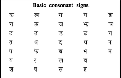
4. In contemporary Devanagari script, there are 13 vowels and 33 consonants.
Fig. 2.1: 13 Vowels of the contemporary Devanagari script
2.2 Smoothing and Filtering
Smoothing is the process that involves removing noise from a data set by
averaging the data points with their neighbours. Smoothing and filtering are two terms
that are used interchangeably, since smoothing brings about a filtering effect by reducing
the high frequencies in the data and strengthening the low frequency content of the data
set.
Before we go deeper into the processes and techniques employed in modern
systems (that process live signals or stored data), it would be appropriate to induce to the
lay reader some sense of the nature of the very problem dealt to the processing system –
which in this case for a recognition system is the presence of unwanted randomness in
data points, which lumped together are termed “noise”. Stemming from the more
common usage of the word noise in the scenario of auditory perception, one might be
compelled to draw the analogy (much rightly in this case however) of the hampering
caused by the unexplained disturbances to the audibility of the more important pieces of
sounds, which could range anywhere from important conversation, a lecture, all the way
up to music and just about anything that is generated for a purpose, and not by a flicker of
randomness.
Now, the conceptual similarity of noise in the realms of any statistical data is not
different at all. It is the same random variation caused amongst the data which makes it
extremely hard to tell the portion of data that was meant to exist in the record – which
could be a 2D capture (image) or a raster of coordinates – from the randomly added data
rational one. It is this feature that is thoroughly undesirable, leading to all the data
muffling, and has to be removed before any processing can take place – just to ensure
that the effort of the processing system works on the right data (that is meant to be
processed in the first place) and not on the muffled sections.
A very logical way of dealing with these statistical variations in the data points is
to get rid of all conspicuous peaks and dents in the smooth flow of the data, by averaging
each data point with its neighbouring points and replacing the data point with this
average, where the number of neighbouring points is defined by a term called “span”.
This definition of the moving average filter ensures that the response of the smoothing is
equivalent to a low pass filter and it can be described by the difference equation [3]
X smoothed (i) = (2N+1)-1*[x (i+N) + x (i+N-1) + … + x (i) + …... + x (i-N)] ….
(2.1)
Where, X smoothed (i) is the smoothed value that replaces the ith data point x (i) and
(2N+1) is the length of the span (Lspan). There are rules that need to be followed
while applying the moving average filter.
1. The length of span (2N+1) should be an odd number to make sure there are an
equal number of points (N) on either side of the data point to be smoothed.
2. The span is adjusted for the points that cannot accommodate the specified
number of points on either side. These are the few initial and end points of the
New Lspan = 2 (min (N,a,b)) + 1
…..(2.2)
Where, a is the number of points on the left side of the data points and b is the
number of points on the right side of the data points.
3. The end points are not smoothed as the length of span cannot be defined for
these points.
2.3 Discrete Cosine Transform (DCT)
The Discrete Cosine Transform (DCT) is a transform that represents any signal as
a summation of cosines that oscillate at different frequencies. The algorithm for DCT was
developed by N. Ahmed et. al [4] and was posed as solutions to the problems of
dimensionality reduction in pattern recognition and Wiener filtering, the two most
popular areas that are catered to by a class of orthogonal transforms such as Discrete
Fourier Transform (DFT), Haar Transform, Karhunen-Loeve transform (KLT) and the
Slant Transform (ST).
In the area of machine learning or pattern recognition, the dimensionality of the
data needs to be reduced. The orthogonal transforms provide a method of transforming
the data in pattern space to a space with reduced dimensionality which is known as the
feature space of the transform. These transforms are usually noninvertible since they
The Wiener filter is used to filter out the noise from a signal by comparing the
signal to an estimated noise-free version of the same signal. Orthogonal transforms are
used to calculate the filter matrix that needs to be convoluted with the noisy signal in
order to obtain the filtered output, since the filter matrix calculated using these transforms
results in a substantial number of elements having values close to zero. Those elements in
the matrix can be replaced with zeros thus reducing the number of multiplications and
additions in the convolution process. We will not go further into the application of DCT
in the field of Wiener filtering and turn our attention to the definition of DCT and how it
fares compared to other popular orthogonal transforms.
Given N real numbers x1, x2, ..., xN, the DCT of these numbers are defined in
different ways with slight modifications, producing the transformed DCT co-efficients
X1, X2, ……, XN
DCT – 1
This definition of DCT of N real numbers makes it equivalent to the DFT of 2N-2 real
numbers with even symmetry.
This is the most popular definition of DCT. DCT of N real numbers is equal to half of
DFT calculated on a series of 4N real numbers which is obtained by replacing every even
indexed element by zero and extending the series to make it even symmetric.
DCT – 3
This definition of DCT – 3 is the inverse of the DCT defined in DCT – 2.
DCT – 4
This DCT is also known as Modified Discrete Cosine Transform (MDCT)
As can be seen from these definitions, DCT of any series of real numbers can be
calculated based on DFT of the same series with slight modifications. There are
numerous algorithms that make use of this property of DCT, thus reducing the
complexity of DCT computation by employing Fast Fourier Transform (FFT) algorithms
such as Cooley-Tukey algorithm, Prime-factor algorithm or Rader’s FFT algorithm. The
FFT algorithms, themselves, have a complexity of O (N log N) and the algorithms for
fast computation of DCT using FFT have an added complexity of O (N) for pre- and post
directly – without the aid of FFT, which employ the classic method of factorization of N
for reducing the computational complexity to O (N log N).
Before we wrap up our section on DCT, we need to look at why DCT acts as a good
signal compression tool and how good the tool is compared to other tools available out
there. A thorough mathematical comparison of DCT with other orthogonal transforms
such as KLT, Haar, Fourier and Walsh–Haddard based on variance and rate distortion has
been made by N. Ahmed et. Al [4]. If we have a look at the comparison (See Fig. 2.3 and
Fig. 2.4), it becomes clear that DCT is closer to KLT in terms of its variance distribution
of transform co-efficients and rate distortion criterion. The definition used by the authors
is DCT – 2.
From the definition and performance of DCT with respect to other transforms, we can see
that DCT not only acts as a good feature extraction method and dimensionality reduction
technique, it also performs better than most other transforms and is as close to the optimal
transform KLT as could be possible [6]. However, when the complexity of computations
Fig. 2.3: Transform domain variance; M = 16, ρ = 0.95. [4]
2.4 Artificial Neural Network (ANN)
An Artificial Neural Network (ANN) is a network of neurons that acts as a
statistical tool to relate inputs to outputs and recognise patterns in data .It was initially
designed to emulate the various processes of the biological neural system and a neuron
model that is an abstraction of the complexity of a real neuron was developed. However,
over a period of time it has evolved to be employed in a variety of applications such as
cognitive psychology, regression analysis and pattern recognition. In this section, we
discuss the role of neurons as building blocks of ANN, the mathematical model of ANN
and its application in the field of pattern recognition. As a pattern recognition tool ANN
helps in classifying classes that are not linearly separable as will be explained later.
An artificial neuron, which is the building block of ANN, consists of inputs, a
summing junction and an activation function; in its most basic and popular form (Fig.
2.5).
The inputs are x1, x2… xp which get multiplied by their respective synaptic
weights w1, w2, …. wp. The summing junction has a bias of value b and its input is
always 1. The summing junction sums all its inputs to give the input (n) to the activation
function. The activation function is a non-linear function that computes the output (a) of
the neuron. The output of the neuron can be expressed mathematically as
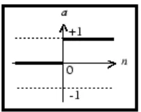
The transfer function can be seen as a limiting function that dictates the output of the
neuron based on the input to the transfer function (n). The most basic transfer function is
the threshold function which gives an output of 0 if n is less than a threshold (usually 0)
and an output of 1 if n is greater than or equal to the threshold. (Fig. )
Fig. 2.6: Threshold transfer function (with threshold value = 0)
There are other different types of transfer functions and the most popular ones are
linear, log-sigmoid and tan-sigmoid. The activation-output characteristics of these
Fig. 2.7: Transfer functions: a). Linear transfer function, b). log-sigmoid function, c). tan-sigmoid function
The weights and the bias are the adjustable parameters of the neuron, and we can
obtain a particular output for a specific combination of weights given a specific set of
inputs. The neuron can be made to behave in some desirable and interesting way by
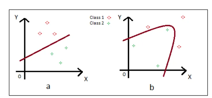
varying these parameters. However, the limitation of an artificial neuron is its ability to
classify only linearly separable classes. The difference between linearly and non-linearly
separable classes is best shown in Fig. 2.8.
.
Ever since the inception of artificial neuron by McCulloch and Pitts [33], various
simple and complex networks consisting of multiple neurons were developed. A network
of neurons (ANN) was necessary for the classification of non-linearly separable classes
and the deployment of these ANNs lead to the development of algorithms that could
compute the weights and biases of the multiple neurons involved. ANNs were unique
since they provided the possibility of learning and in order to realize the learning
functionality in ANNs, special learning algorithms were engineered that could not only
adjust the weights and biases but also could do so taking into account the relationship
between desired outputs in response to a set of inputs.
The ANNs differ in their choice of transfer function, topology and learning
algorithms. In this section, we will be focussing on one particular kind of ANN called the
feed-forward network since it is the most common network and other models are based
on it. This is in contrast with the other type of neural network topology which is the
recurrent neural network with feedback loop. The learning algorithm discussed is the
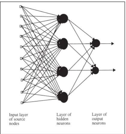
resilient backpropagation algorithm. An ANN may have one or more of layers with layer
containing multiple neurons. Most neural networks have two layers of neurons with the
first layer called hidden layer and the second layer called output layer. These two layers
are preceded by the input layer which consists of just inputs and no neurons (Fig. 2.9).
The network receives inputs from the input layer and the output of the neural network is
available at the output layer.
These feed forward neural networks are also known as multilayer perceptrons
Rumelhart [34] accomplishes the design of a feed forward neural network. Before we dig
deep into the workings of the back propagation algorithm, it becomes imperative at this
point that we discuss a little bit more about the concept of learning. The learning process
is necessary for the network to acquire desired knowledge and apply this process on its
inputs and provide us with the correct outputs. As mentioned earlier, this necessary
knowledge is stored in the set of parameters (weights and biases) of all the neurons in the
network. On a broad level, the learning process has been classified into two types:
• Supervised learning that involves training the network with a set of
training samples
• Unsupervised learning that involves classifying models based on
unlabelled data.
Let the set of training samples in supervised learning be denoted by P, which is a set of N
pairs of samples.
T = {(x1, y1), (x2, y2)… (xN, yN)} ….(2.9)
Where,
x1, x2 .…, xN are all input vectors and belong to input vector space X
y1, y2 … yN are all desired output vectors for the respective input vectors and
belong to output vector space Y
N is the number of such samples
As part of supervised learning, the neural network is trained with these sample
pairs either on a one-by-one basis or in a batch and after each input-output pair pass (xi,
yi), the parameters of neurons in hidden and output layer are computed so that the actual
output (ai, where i = 1,…, N)of the neural network is close to the desired output (yi,
where i = 1,…, N) based on a performance measure such as the mean square error
defined as
𝐸 = !! ! (𝑦!− 𝑎!)!
!!! …(2.10)
The mean square error is the designated cost index that needs to be minimized
over the complete set of training samples and the resulting neural network represents the
function f : X -> Y, which could be described as the optimised classifier function. For
to be moved through all possible values in proportion to the gradient of the error (E). The
gradient descent algorithm that finds out the local minimum of any function is used for
this very purpose. The delta rule employs the gradient descent algorithm for obtaining the
weights of neurons in a single layer perceptron. If, however, the network involved is a
multilayer perceptron then the generalised version of the delta rule – backpropagation
algorithm is employed. Thus, we can note that by being an algorithm that is used by
multilayer perceptron training, backpropagation algorithm needs to have the capability to
handle adjustments in a large number of neurons in very complicated network topologies.
Backpropagation algorithm has 2 broad steps –
1. Forward phase: In this step, parameters (weights) of the neurons in the
network are fixed and inputs are applied at the input layer and the
corresponding outputs are calculated. This step also includes calculation of the
error
ei = yi – ai ….(2.11)
where, yi is the desired output vector and ai is the actual observed output
vector for a given input vector xi.
2. Backward phase: The error calculated in the forward phase is propagated in
the backward direction through all the neurons in both output and hidden
layers. It is in this stage that the weights of the neurons are adjusted by using a
In sequential mode, the forward phase is implemented on each input-output pair
individually and in batch mode, the forward phase is carried out on a sizeable batch of
input-output pairs. In both cases, the error function E is determined using Eq. (2.10) and
is treated as the cost function to be minimized.
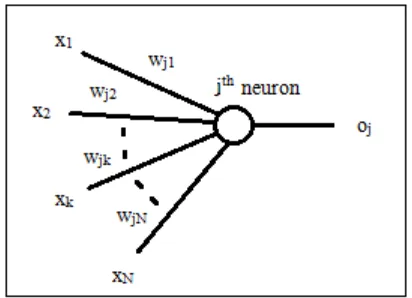
Let us consider the jth neuron in the hidden layer of Fig. . The input to this neuron
is the actual input vector to the neural network xi (i = 1, …, N) and let the weight matrix
of the synapses connecting the inputs to this neuron be wij. The error function E needs to
be minimized with respect to each of the weights in the weight matrix and in order to
accomplish that, we need to consider the partial derivative of the error function with
respect to each weight in the weight matrix. A simpler figure (Fig. 2.10) is provided for
the convenience of the reader.
Fig. 2.10: A magnified view of the jth neuron
Let us consider the partial derivative of E with respect to the weight that connects the kth
element in the input vector to the jth neuron (wjk). Applying the chain rule, we obtain the
Where, zj is the weighted sum of inputs for the jth neuron and xk is the kth element of the
input vector. Employing the general rules of differentiation, it can be shown that
Where, tj = desired output for jth neuron
oj = actual output obtained for jth neuron
Substituting Eq. (2.13) and Eq. (2.14) in Eq. (2.12), we obtain
Deriving the delta adjustment to weight wjk from Eq. (2.15), we obtain
The term η is called the learning rate of the backpropagation algorithm. Thus, the weight
As we can see, the weights are updated in the opposite direction to the sign of the
gradient, making sure the error decreases in steps of η with every weight update. The
choice of learning rate η determines how fast the local minimum is reached and also
affects the quality of learning. The forward and backward steps are repeated for all
training samples or till the network has met satisfactory performance standards.
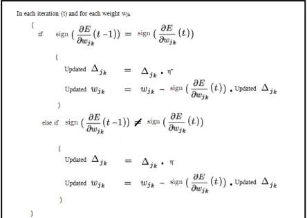
Many algorithms have been proposed for adapting weights in neural networks that
are based on backpropagation algorithm. The resilient backpropagation (Rprop) is one of
the best methods that could be used for achieving batch learning in MLPs. The Rprop
considers only the sign of the partial derivative of the error function and not on its exact
value, thus making it an appropriate, fast and easy algorithm for implementing in the case
of noisy error function.
In Rprop algorithm, the weight adjustment equation is given by
Thus the direction of the weight update is dependent only on sign of the partial derivative
and not on its absolute value. Also, the weight is updated in steps of Δjk, which is based
on changes in the sign of the partial derivative. Depending on whether there is change in
the sign of the partial derivative, Δjk is multiplied by a value of η+ (η+ > 1) or a value of η-
Fig. 2.11: An easy-to-follow algorithm of Rprop method is provided for enhanced readability.
This chapter on preliminaries touched upon all necessary concepts required to understand
the premise of the thesis. This section was aimed at familiarizing the novice reader with
CHAPTER III
REVIEW OF LITERATURE
3.1 Basics
Handwriting recognition (HWR) is the process of obtaining handwritten material,
either in the form of scanned images of handwritten documents or in the form of spatial
co-ordinates of the hand movement of users, and developing it into a form that can be
recognized by a computer or any text based application. Early developments in the area
of handwriting recognition were mainly aimed at aiding the blind and also improving
interface between human and the computer, thus bringing about increased functionality
and user-friendliness in computers.
3.2 Offline Vs Online Handwriting Recognition
As discussed, handwriting recognition can be either offline or online depending
on whether the input is scanned and digitized copy of handwritten documents or x-y
co-ordinates of the hand movement - for example through a motion based sensory screen of
a computer, respectively. Offline handwriting recognition is a specific case of “Optical
Character Recognition” (OCR). There are positive and negative points associated with
both methods of recognition. OCR is well suited in situations where the handwritten
material is already available in document form or when the range of characters is already
Online handwriting recognition, on the other hand, proves to be a better choice
when the handwriting needs to be recognized as the character is being written. A deeply
descriptive, objective and comprehensive comparison of offline and online handwriting
recognition methods on Latin alphabet has been done by Rejean Plamondon and Sargur
N. Srihari [7]. In their landmark survey, they have clearly elucidated the various
differences, pros and cons of online and offline HWR. Besides having lesser data storage
requirements than offline recognition, online recognition provides better recognition rates
as well. The memory requirement for online recognition of an average English word is
about few 100 bytes, at a sampling rate of 100 samples per word, whereas for offline
recognition, it is about few 100 kilo-bytes, sampled at a rate of about 300 dots per inch. A
recognition rate of 78 percent has been reported for offline word recognition with 1000
word lexicon [8], in comparison to a recognition rate of 80 percent for online word
recognition with 21000 word lexicon [9]. Though better recognition rates have been
reported in both offline and online HWR, online recognition algorithms outperform
offline handwriting recognition methods in terms of data memory requirements and
recognition rates, given the same lexicon size.
3.3 Pen Computing and Tablet PCs
An important precursor for online HWR is the availability of tablet PC or
digitizer, which is collectively known as pen computing. A tablet PC or digitizer serves
as the interface to collect the time ordered 2-Dimensional co-ordinates of the user's hand
movement and employs a pen (stylus), and a touch sensitive screen, that collects and also
technology spans over a century and a detailed discussion of it by Andre Meyer [10] and
by Jayashree Subrahmonia and Thomas Zimmerman [11] present a complete and detailed
picture of the then state-of-the-art. In 1888, Elisha Gray was awarded a patent for
inventing a device that could capture handwriting and thus began the exploration that
spewed many devices that could accurately acquire and store handwriting. All major
corporations have produced their own versions of tablet PC and most commercially
available ones make use of top choice handwriting recognition algorithms. A pen
computing device basically consists of a tracking technology (magnetic, electric,
ultrasonic or optical tracking) that determines the position of the stylus on the screen.
Most modern tablet PCs use one or a combination of these tracking technologies.
This thesis tries to highlight the salient patches of the survey of pen computing in
[12], such that the entire spectrum of pre-1990 research is shone light upon – without
entering into the specifics of surveyed ideas that are obsolete or are close to being so. The
authors point to the inception of pen-trajectory tracking in the 1950s, immediate interest,
and a dip in attention in the 1970s, and revival a decade later. It is to be noted that this
fluctuation in interest and attention can be attributed to the technological differences, by
which I mean the 1960s and '70s definitely lacked the power of computers, tablet PCs,
touch-screen hand-held devices, and efficient algorithms for quick processing. Online
handwriting recognition has survived the test of time for the simple reason that a whole
lot more data is available for recognition systems than an offline snapshot of handwriting
can ever provide. It is needed to expand upon the ideas of pen computing and trajectory
Dimond's “Stylator” [13] has been the earliest documented tablet digitizer, the
most popular one being the RAND table [14]. These spurred the initial thrust towards
online handwriting recognition research. Before I move on to the actual research
surveyed in [12], it is imperative to introduce the two popular technologies used to build
digitizers. This will serve as a background with which to better understand the conditions
prevalent for the researchers of the past. As of 1990, electromagnetic/electrostatic and
pressure sensitive were the two dominant technologies.
The former category of tablets (electromagnetic/electrostatic) had regularly
spaced x and y grids of conductors. The stylus tips had a loop of wire. When the grid (or
the loop) was excited with an electromagnetic pulse, the loop (or the grid) would detect
the induced voltage or current as a sine wave. The tablet conductors were searched to
point to the pair closest to the loop, and the precise position between these two
conductors was determined by interpolation. As one can expect, the recognition gets
more accurate with higher density of the regularly spaced on-tablet conductors.
Pressure-sensitive tablets were a little different, in that the tablet makes use of two
types of layers – one conductive, and one resistive. The spacing between any conductive
layer and the corresponding resistive layer is the key for operation, and it is where the
concept of vertical pressure comes in. In a pre-specified direction (usually along either
the x- or the y-axis), some electric potential is applied across one of the resistive layers.
By applying pressure on the stylus, the user would enable the conductive layer to make
contact with the resistive layer, picking the voltage from the latter, thus picking the
required of the stylus is the pressure. This eliminated the need to find a special type of
stylus for the tablet, and it has been a huge advantage since.
The authors also discuss briefly other sensing techniques, like the acoustic and
optical sensing methods – and these will be skipped from the survey in this thesis.
However, it will be mentioned that the authors wrap up the section on digitizers by
alluding to the dawn of transparent tablets (the earliest of which dates back to 1968 [15])
– enabling the user to use the same tablet for input as well as output, at the same time.
With the different tablet digitizer technologies behind us, it is time to move on to have a
look at the pre-1990 perception of handwriting properties and mechanisms of recognition
based on these properties. It is at this point that the fact that we are dealing with online
handwriting becomes more important and useful. Handwriting when recorded as written
(which is of course the essence of online capture) can be viewed as a series of strokes,
tagged with their time-stamps – in order to properly stack the coordinates of each stroke
in a timely manner so as to preserve handwriting causality intact.
3.4 General Online Handwriting Recognition
The work done under online HWR is vastly focused on Latin alphabet and
numeral set. Interest in online HWR commenced in early 1950s, largely due to the advent
and advancement in pen computing. Important contributions to the field of online HWR
were made in 1960s and 1970s which were a result of availability of better tablets PCs,
algorithms differed in the way the researchers chose to solve various issues that act as
obstacles to the achievement of perfection in handwriting recognition.
We can easily note that all online HWR algorithms work on the basic assumption
that different handwritten characters in any given script have a high degree of
decorrelation. While this is a useful property, another characteristic of handwriting that is
at least as useful if not more is that the handwriting samples of the same given character
in any particular script are highly correlated. A deep understanding of the variability in
handwriting is essential if we intend to build better and efficient HWR systems and
readers are referred to [16] for a thorough discussion of the variability effects in English
handwritten script. As part of the literature survey on online HWR, I would like to
include significant work in all steps of HWR – starting from pre-processing all the way
up to final classification. To that end, let us begin an overview of important past work
pertaining to the pre-processing steps.
Though this thesis work does not require segmentation between characters as well
as segmentation within each character, it is still required to showcase all crucial scholarly
work on segmentation so that the continuity, discussion flow, and completeness are all
kept intact. Earliest efforts in segmentation were in the form of obtaining the horizontal
distance between the characters [17] or by providing a certain amount of time for the user
to complete writing the character. Most of the times, users were asked to write characters
in certain boxes meant for each character which is akin to character recognition. Many of
the recent published works talk of two dimensional separation of characters [18] or use of
Smoothing and filtering of the handwriting samples are vital pre-processing steps
that have been implemented in various ways. The most commonly used method for
smoothing is averaging of the sample points with its neighbours [20]. As part of filtering,
most researchers resample the data points so that consecutive points are all equally
spaced [20]. To bring about various types of normalizations, different algorithms have
been suggested. Some of the examples are: deskewing algorithms that are carried out to
de-slant the characters, size normalization algorithms in order to reduce or expand
characters from different users which tend to be of different sizes to the same size as the
case may be, stroke length normalization equalises the number of sample points in each
stroke so that all strokes have uniform length [21].
After obtaining the handwriting samples and applying all necessary
pre-processing algorithms in order to obtain smoothed, filtered and normalized data points,
the samples need to be reduced to a set of non-redundant, yet sufficiently informative
data samples. All methodologies that are aimed at achieving dimensionality reduction are
basically different forms of feature extraction methods. Anyone, who sets out to actualize
handwriting recognition, has a varied collection of feature extraction approaches to
choose, ranging from static features and dynamic features, a combination of both static
and dynamic to those features that are representation of the data samples in some other
domain. The choice that one makes is usually influenced by factors such as the language
and script in question, the choice of classification method and the ease with which certain
features can be extracted from the samples. Binary features are mainly used as part of a
decision tree so that each branch of the tree corresponds to a particular combination of
conjunction with some classification method such as clustering analysis that clusters
those features into a set of groups.
With each character being represented by extremely efficient feature arrays, we
are faced with the challenge of developing a classification method that sorts these feature
vectors into one character class among all character classes in the script. In simplest of
terms, classification is a sub-problem in pattern recognition, in which, given an input
vector the process involves matching this input vector with an output label. These
classifiers are statistical in nature, which means these classifiers are able to detect certain
characteristics, attributes or properties of classification based on a large number of
observations with known output label for each input vector. This type of classification is
also known as supervised learning. Linear classifiers such as Fischer Linear
Discriminant, perceptron and others such as Artificial Neural Networks (ANN) [22],
Support Vector Machines (SVM) [23] and k-nearest neighbour are some of the classifiers
that have been used extensively by various researchers.
3.5 Devanagari Online Handwriting
After a detailed perusal of the state-of-the-art techniques in online HWR in
English language, let’s turn our attention to the core of this thesis topic – Devanagari
script online HWR. Though a huge amount of work has been done on offline handwriting
recognition for Devanagari characters, publications focused on online Devanagari
Scott D. Connell et. al. [24] were the first few ones to work on this area and their
seminal work on “Recognition of unconstrained online Devanagari characters” in 2000
brings to light the various issues involved in online Devanagari HWR. They have
implemented a method which uses 5 classifiers with both online and offline features.
Offline features refer to those features extracted after considering the character as whole
rather than calculating the features based on the sample points that are collected from the
handwriting. Their resultant accuracy rate of the five classifiers combined is reported to
be 86.5 %, with the individual classifiers themselves providing much lesser accuracy
rates.
In chronological order, the next work that could be mentioned as part of a survey
of the developments in online Devanagari HWR is by A. M. Namboodiri et. al. [25]. The
authors propose a method to classify a given online script into one out of 6 scripts, one of
which is Devanagari. The method used 11 spatial and temporal features extracted from
the strokes of the words and attained an accuracy of 87.1 percent on a database of 13,379
words. Although, this piece of work on classifying words into scripts has no implications
and results that could be used as a reference for the work on online Devanagari HWR, it
throws ample light on the various features that could be used for classifying Devanagari
characters.
Niranjan Joshi et. al [26] specify a system that uses structural features such as
mean (x, y) values, positional cues and directional codes at the stroke level and a test
vector is developed based on these features. The system uses subspace method for
of N eigenvectors. The test vector is assigned to that class whose basis vector has the
smallest orthogonal distance from the test vector. The most notable result reported is an
average accuracy of 93.05% on a set of 100 frequently occurring characters.
A stroke-based recognition system using Hidden Markov Model (HMM) has been
proposed by Abhimanyu Kumar and Samit Bhattacharya [27]. Their work on recognition
of isolated Devanagari characters has been carried out to be implemented on the iPhone.
The authors have created 42 stroke classes, and one HMM is constructed for each stroke
class. The first round of stroke classification results are fed into a second round of
classifiers, along with look-up tables. Six scalar features indicate the size and shape of
each sub-stroke. However, the authors sign off with an end-of-paper discussion, and no
actual results are presented to the reader. This makes the assessment of their approach
very ambiguous and speculative in terms of accuracy and recognition rate, as the number
of samples and degree of variety keep mounting.
The recognition rate, time required to train the system and number of samples
used per character for testing are some of the criteria that can be utilized to compare the
performances of these above mentioned scholarly work. The recognition rate which is the
ratio of number of correct classifications to the total number of training samples, gives a
measure of how well the system is performing in general. The next performance criterion
is the training time which is the total time required to train the network to correctly
classify all the training samples. The number of samples per character class used for
training the system is also an essential performance criterion since it provides an insight
performance measures, there are parameters that take into account details such as run
time and memory requirements. Any scholarly work survey on HWR is not complete
without a comparison of the published algorithms based on these criteria. However, we
can notice that the authors that figure in the technical survey show no form of
conformance to the afore discussed performance criteria, but rather stick to exposition of
the bare minimum information that is open to further inference and investigation – such
as the overall recognition rate and the number of samples per character used for testing
their algorithms.
This concludes our fairly extensive survey on the state-of-the-art, and the work
that has led us up to it. We are now at a stage where we can fully appreciate the problem I
have been working on, the complications involved, how it differs in approach and
solution to the scholarly work we have just finished surveying, and finally how I solve
CHAPTER IV
DESIGN AND METHODOLOGY
4.1 Overview of the Proposed Methodology
We have seen quite a few times that handwriting recognition is a capability
linked, in this context, to any programmed module that resides in a processing unit. This
is the core of the system to which the recognition capability is attributed. However, much
like the role the CPU has come to play in the whole computing experience, the program
module is part of a bigger system. It is, more often than not; wrong to focus on the core
unit sidelining the peripheral units. In fact, it is not uncommon at all for the performance
and design of the peripheral units of a typical recognition system to bear a rather direct
impact on the overall ability to recognize handwriting correctly and efficiently.
It is with this background that we need to look at the overall development of our system,
going sequential – as if we are tailgating the data to be processed (or more specifically in
this case, the handwriting sample to be recognized). This way, it is easy for the reader –
and more importantly for the designer – to expect and be prepared for the alteration that
awaits the data next.
Once the nature of the system is decided upon, one of the first things to be acted
upon is the nature of the data. In this case, the system that is being built is a recognition
system for online handwriting characters belonging to the ancient Indo-European heritage
script, Devanagari. This immediately dictates the input mechanism, and the policies to be
employed thereof. While mechanism entails the procedure and process of taking in the
in the process of data acquisition – in order to bring about numerous features to the
system being built. These features can range from ethnic invariance, robustness, speed
invariance, angular invariance, and immunity to distortion, all leading the system toward
one ultimately desirable state of user-independence. In more explicit terms, what this
means is that the data has to be tuned in a way that the system would have no difficulty in
recognizing characters from a secondary data set (usually termed the “test set”) which has
no intersection with the primary data set (commonly referred to as the “training set”) –
regardless of the variation that finds expression as a function of several attributes of the
database contributors – leaving the legibility of the written script as the only concern for
successful recognition.
The process of thus preparing the data in a way such that the system functioning
is rendered insensitive to user-dependent variances, environment-dependent fluctuations,
and randomness (whose capture happens only in posteriori measurements, leading to
well-developed statistical quantifications) is an art – that goes by the name
pre-processing.
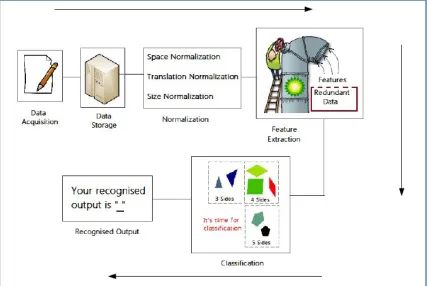
The various stages of readying a potential handwriting recognition system goes
far beyond the core module, often starting at data acquisition (either afresh or via an
accredited database), routing through storage and pre-processing, right to the
identification of feature cruxes and their extraction, all the way up to the design of the
classification unit at the core – which, akin to a two year-old kid, learns to tell one class
of data from another, based on the featured identified in the previous step.
Fig. 4.1: The developmental stages of the handwriting recognition system – adopted in the work.
The various stages in the HWR systems are
1. Data Acquisition
2. Data storage
3. Normalization
4. Feature extraction
4.2 Nature of Data, Acquisition and Storage
The above steps are common to any recognition system. Specifically, in our case,
steps 1 and 2 are merged into one block. It is only natural to do this since the data
acquired has to be taken care of, either in terms of processing or storage. Immediate
processing of the acquired data forces the system to turn into a real-time entity, which is
not what this work of mine is intended for. In handwriting recognition systems, there are
steps that typically need to be followed before the actual processing can take place. The
data accumulation can be overwhelming for any real-time system (with minimum
memory) while the system readies one batch of data for actual processing. It is due to this
simple reason that handwriting recognition (and many other pattern recognition and
image analysis) systems are seldom made real-time.
Once we come to the decision that the system is not real-time, then we need to
take care of the data accumulation, such that the integrity and content of the data – in its
entirety – is not lost. This calls for a proper storage arrangement. Therefore, it is vivid as
to why any handwriting recognition system designer would naturally want to merge the
steps of data acquisition with the imminent and inevitable step of data storage.
Before discussing data acquisition at any length, it is a good idea to understand
the type of recognition system – as the nature of the system has a direct impact on the
nature of the data being fed. Most of the work, as we have seen during the literature
survey chapter, focuses on the recognition of script which is printed or handwritten some
time ago, on a non-electronic medium. Now, what that means is that the there is no
usually termed “offline” data. The most widely found examples of offline data are
images/pictures of written/typed script. Often in the world, offline data is what we have
easier access to – be it pages from a book, an old handwritten document, an unsigned
letter, or an ancient manuscript. We don’t have control over the type of data. But in the
modern age, the electronic presence is growing, allowing one to think about having more
control over the data being acquired.
Offline data samples have their share of disadvantages. Perhaps the best way to
drive home the major disadvantage of offline data is through the following example:
Consider two persons – Ronald and Donald. Ronald is an influential man, with the real
authority to sign an important document of a reasonably high impact. Due to
discretionary reasons, Ronald wouldn’t sign a particular document. In Ronald’s absence,
Donald, who is a fraudster, carefully signs the document (which Ronald had declined to
sign). After Donald finishes signing the document, it looks exactly identical to Ronald’s
signature. Now suppose this signature of Donald’s signature is captured offline, then it is
nearly impossible to bring Donald to justice. However, had Donald’s forgery been
captured electronically, one could have access to the temporal features of Donald’s
signature. The pressure of the strokes, the timing, and the speed of sub-strokes are all
collected in an electronic acquisition of data. This type of data is termed online.
The above example illustrates the advantage of dealing with online data as
opposed to offline data, due to the availability of temporal characteristics in the former
The example of Ronald and Donald has been made up for the sake of illustration.
However, the problem described herein is real. It has been a recurrent problem through
the course of history, as we shall see with one real example below.
The forgery shown in Fig. 4.2 below is not the best forgery one could imagine,
but it comes pretty close to the original. The concern grows in cases where the visual
distinction between two writings (signatures and regular writing alike) is harder to make
than the example below.
Fig. 4.2: A real signature, and its forged version: offline recording.
Tom Davis (of the University of Birmingham) has an interesting analysis of this
forgery [28]. Tom opines, “The forgery is quite good, both in line quality and letter
formation, and at first sight looks very convincing. But look at it closely. Firstly, the
laudable concentration on line quality has led to a gross error, in that an extra minim has
straight lines and corners, which is very characteristic of forgery. And, in the case of the
lower loop of the final /y/, the reverse has occurred: a curve in place of an angle and
straight line. Then look at the end of that stroke: in the genuine signature the pressure of
the pen reduces gradually, while in [the forged version] the line ends abruptly, no doubt
with relief; a failure of concentration at the end of the job.”
The case has been made, intuitively at the least, for the choice of using online data
for training and testing the HWR system. The logical continuation of the choice (of the
nature of data) is the specification of the acquisition module of the system.
4.2.1 Need for building a database
It may seem to the reader that the obvious choice for acquiring data is to use a
database of handwriting samples – along with the knowledge of the relevant methodology
behind the build-up of the database being considered. What adds an extra level of
challenge to this work is that there is no readily available database for Devanagari
characters, unlike the Yale B/Extended Yale B/CMU-PIE databases that exist for human
faces, or unlike the USPS/MNIST digit databases. The direct, unavoidable, implication is
that it becomes a responsibility to populate a decent sized database for isolated
Devanagari characters, from scratch.
4.2.2 Building the database: considerations and methodology
Recognizing the importance of this step, we worked out a comprehensive way of
creating this database, in a way that a variety of writing styles – in the right number – are
A quick detour is essential to set the premise for the strategic development of our
unique comprehensive database. The protagonist, resorting to personification for lack of a
better inanimate qualifier, of this thesis is the script, Devanagari. Devanagari, as
explained earlier, is a rich script of the Indo-European belt, now finding residence mainly
in the Indian languages. The language-script relationship evolves over time, causing the
language to get control over how the script changes to suit the needs of the development
of the language itself. In other words, what sets off as a common script for say, five
languages, is sculptured by time and the respective language into five similar scripts of
common ancestry.
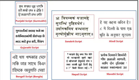
The original Devanagari script is known to most closely resemble the four scripts
in the right big box in Fig. 3.3. Within this big box, the four scripts are enormously
similar, with just very minor variations. However, the other boxes carry scripts (Punjabi,
Gujarathi, and Bangla) that have drifted farther off from the parent Devanagari script.
The unique thing incorporated in the database is that we have ensured that the influence
of all these script-drifts is taken into account. The people from whom handwriting
samples are obtained for building the database have varied backgrounds. Their linguistic
origins include Hindi, Gujarathi, Marathi, Punjabi, and Bangla. The scripts of these
languages, as we saw above, are off-shoots of Devanagari. We have also taken
Devanagari samples from people whose native script has no connection with Devanagari
at all (like Kannada, Tamil, Telugu, and Malayalam).
The variety that has been created in the database makes sure that the handwriting
recognition system is immune to the influence of the native script (of the handwriting
sample contributor).
Let us quickly touch upon the concept of layering, which gains relevance in this
context. How entries are arranged in the database is that the samples are spread from
contributors of various linguistic origins, in recurring layers, so to say.
Fig. 4.4: Layering of handwriting samples from contributors of various linguistic backgrounds, making the database uniform and randomly interspersed.
The rationale behind adopting such a scheme as layering is to make sure that even
a small section of the database is not biased towards any particular script-influence on the
writing style of the Devanagari characters. This way, the results of testing is uniform and
largely independent of the section of the database upon which the testing is carried out.
![Fig. 2.4: Rate versus distortion for M = 16 and ρ = 0.9 [4]](https://thumb-us.123doks.com/thumbv2/123dok_us/1434364.1175873/24.612.176.473.79.328/fig-rate-versus-distortion-m-and-r.webp)