Particle Filtering Applied to Musical Tempo Tracking
Stephen W. Hainsworth
Department of Engineering, University of Cambridge, Cambridge CB2 1PZ, UK Email:[email protected]
Malcolm D. Macleod QinetiQ, Malvern, WR14 3PS, UK Email:[email protected]
Received 30 May 2003; Revised 1 May 2004
This paper explores the use of particle filters for beat tracking in musical audio examples. The aim is to estimate the time-varying tempo process and to find the time locations of beats, as defined by human perception. Two alternative algorithms are presented, one which performs Rao-Blackwellisation to produce an almost deterministic formulation while the second is a formulation which models tempo as a Brownian motion process. The algorithms have been tested on a large and varied database of examples and results are comparable with the current state of the art. The deterministic algorithm gives the better performance of the two algorithms.
Keywords and phrases:beat, tracking, particle filters, music.
1. INTRODUCTION
Musical audio analysis has been a growing area for research over the last decade. One of the goals in the area is fully auto-mated transcription of real polyphonic audio signals, though this problem is currently only partially solved. More realistic sub-tasks in the overall problem exist and can be explored with greater success; beat tracking is one of these and has many applications in its own right (automatic accompani-ment of solo performances [1], auto-DJs, expressive rhyth-mic transformations [2], uses in database retrieval [3], meta-data generation [4], etc.).
This paper describes an investigation into beat tracking utilising particle filtering algorithms as a framework for se-quential stochastic estimation where the state-space under consideration is a complex one and does not permit a closed form solution.
Historically, a number of methods have been used to at-tempt solution of the problem, though they can be broadly categorised into a number of distinct methodologies.1 The oldest approach is to use oscillating filterbanks and to look for the maximum output; Scheirer [7] typifies this approach though Large [8] is another example. Autocorrelative meth-ods have also been tried and Tzanetakis [3] or Foote [9] are
1A comprehensive literature review can be found in Sepp¨anen [5] or Hainsworth [6].
examples, though these tend to only find the average tempo and not the phase (as defined inSection 2) of the beat. Mul-tiple hypothesis approaches (e.g., Goto [10] or Dixon [11]) are very similar to more rigorously probabilistic approaches (Laroche [12] or Raphael [13], for instance) in that they all evaluate they likelihood of a hypothesis set; only the frame-work varies from case to case. Klapuri [14] also presents a method for beat tracking which takes the approach typified by Scheirer [7] and applies a probabilistic tempo smooth-ness model to the raw output. This is tested on an extensive database and the results are the current state of the art.
More recently, particle filters have been applied to the problem; Morris and Sethares [15] briefly present an al-gorithm which extracts features from the signal and then uses these feature vectors to perform sequential estimation, though their implementation is not described. Cemgil [16] also uses a particle filtering method in his comprehensive paper applying Monte Carlo methods to the beat tracking of expressively performed MIDI signals.2This model will be discussed further later, as it shares some aspects with one of the models described in this paper.
The remainder of the paper is organised as follows: Section 2introduces tempo tracking;Section 3covers basic
particle filtering theory. Sections4,5and6discuss onset de-tection and the two beat tracking models proposed. Results and discussion are presented in Sections7and8, and conclu-sions inSection 9.
2. TEMPO TRACKING AND BEAT PERCEPTION
So what is beat tracking?3 The least jargon-ridden descrip-tion is that it is the pulse defined by a human listener tap-ping in time to music. However, the termstempo,beat and rhythm need to be defined. The highest level descriptor is the rhythm; this is the full description of every timing re-lationship inside a piece of music. However, Bilmes [17] breaks this down into four subdivisions: the hierarchical met-rical structurewhich describes the idealised timing relation-ships between musical events (as they might exist in a mu-sical score for instance), tempo variationswhich link these together in a possibly time varying flow, timing deviations which are individual timing discrepancies (“swing” is an example of this) and finally arrhythmic sections. If one ig-nores the last of these as fundamentally impossible to analyse meaningfully, the task is to estimate the tempo curve (tempo tracking) and idealised event times quantised to a grid of “score locations,” given an input set of musical changepoint times.
To represent the tempo curve, a frequency and phase is required such that the phase is zero at beat locations. The metrical structure can then be broken down into a set of lev-els described by Klapuri [14]: thebeat ortactusis the pre-ferred human tapping tempo; thetatumis the shortest com-monly occurring interval; and thebarormeasureis related to harmonic change and often correlates to the bar line in com-mon score notation of music. It should be noted that the beat often corresponds to the 1/4 note or crotchet in common no-tation, but this is not always the case: in fast jazz music, the beat is often felt at half this rate; in hymn music, traditional notation often gives the beat two crotchets (i.e., 1/2 note). The moral is that one must be careful about relating percep-tion to musical notapercep-tion!Figure 1gives a diagrammatic rep-resentation of the beat relationships for a simple example. The beat is subdivided by two to get the tatum and grouped in fours to find the bar. The lowest level shows timing devia-tions around the fixed metrical grid.
Perception of rhythm by humans has long been an active area of research and there is a large body of literature on the subject. Drake et al. [18] found that humans with no musical training were able to tap along to a musical audio sample “in time with the music,” though trained musicians were able to do this more accurately. Many other studies have been un-dertaken into perception of simple rhythmic patterns (e.g., Povel and Essens [19]) and various models of beat percep-tion have been proposed (e.g., [20,21,22]) from which ideas can be gleaned. However, the models presented in the rest of this paper are not intended as perceptual models or even as perceptually motivated models; they are engineering
equiva-3A fuller discussion on this topic can be found in [6].
8 Score Tatum Beat Bar Timing
Figure1: Diagram of relationships between metrical levels.
lents of the human perception. Having said that, it is hoped that a successful computer algorithm could help shed light onto potential and as yet unexplained human cognitive pro-cesses.
2.1. Problem statement
To summarise, the aim of this investigation is to extract the beat from music as defined by the preferred human tapping tempo; to make the computer tap its hypothetical foot along in time to the music. This requires a tempo process to be ex-plicitly estimated in both frequency and phase, a beat lying where phase is zero. In the process of this, detected “notes” in the audio are assigned “score locations” which is equiva-lent to quantising them to an underlying, idealised metrical grid. We are not interested in real time implementation nor incausalbeat tracking where only data up to the currently considered time is used for estimation.
3. PARTICLE FILTERING
Particle filters are a sequential Monte Carlo estimation method which are powerful, versatile and increasingly used in tracking problems. Consider the state space system defined by
xk=fk
xk−1,ξk
, (1)
where fk :nx× nξ → nx,k∈N, is a possibly nonlinear
function of the statexk−1, dimensionnxandξk which is an
i.i.d. noise process of dimensionnξ. The objective is to
esti-matexkgiven observations,
yk=hk
xk,νk
, (2)
wherehk:nx× nν → nyis a separate possibly nonlinear
transform andνk is a separate i.i.d. noise process of
dimen-sionnνdescribing the observation error.
The posterior of interest is given byp(x0:k|y1:k) which is
represented in particle filters by a set of point estimates or particles{x0:(i)k,wk(i)}Ni=1, where{x
(i)
0:k, i =1,. . .,N}is a set of
support points with associated weights given by{wk(i), i =
1,. . .,N}. The weights are normalised such thatiN=1wk(i)=
1. The posterior is then approximated by
px0:k|y1:k
≈
N
i=1 wk(i)δ
x0:k−x(0:i)k
AsN→ ∞, this assumption asymptotically tends to the true posterior. The weights are then selected according to impor-tance sampling,x0:(i)k∼π(x0:(i)k|y1:k), whereπ(·) is the so-called
importance density. The weights are then given by
w(ki)∝
px(0:i)k|y1:k
πx0:(i)k|y1:k
. (4)
If we restrict ourselves to importance functions of the form,
πx0:k|y1:k
implying a Markov dependency of order 1, the posterior can be factorised to give
which allows sequential update. The weights can then be proven to be updated [23] according to
w(ki)∝w(ki−)1
up to a proportionality. Often we are interested in the filtered estimatep(xk|y1:k) which can be approximated by
Particle filters often suffer from degeneracy as all but a small number of weights drop to almost zero, a measure of this being approximated byNeff =1/Ni=1(wk(i))2[23]. Good
choice of the importance densityπ(xk|x0:k−1,y1:k) can delay
this and is crucial to general performance. The introduction of a stochastic jitter into the particle set can also help [24]; however the most common solution is to perform resam-pling [25] whereby particles with small weights are elimi-nated and a new sample set{xk(i)∗}N
i=1is generated by resam-plingNtimes from the approximate posterior as given by (8) such that Pr(xk(i)∗ =xk(j))=w(kj). The new sample set is then
more closely distributed according to the true posterior and the weights should be set towk(i)=1/Nto reflect this. Further
details on particle filtering can be found in [23,26].
A special case of model is the jump Markov linear sys-tems (JMLS) [27] where the state space,x0:k, can be broken
down into{r0:k,z0:k}.r0:k, the jump Markov process, defines
a path through a bounded and discrete set of potential states
and conditional upon r0:k,z0:k is then defined to be linear
Gaussian. The chain rule gives the expansion,
pr0:k,z0:k|y1:k
Kalman filter equations given below inSection 5. After this marginalisation process (called Rao-Blackwellisation [28]),
p(r0:k|y1:k) is then expanded as
with associated (unnormalised) importance weights given by
w(ki)∝w
By splitting the state space up in this way, the dimensionality considered in the particle filter itself is dramatically decreased and the number of particles needed to achieve a given accu-racy is also significantly reduced.
4. CHANGE DETECTION
The success of any algorithm is dependent upon the reliabil-ity of the data which is provided as an input. Thus, detecting note events in the music for the particle filtering algorithms to track is as important as the actual algorithms themselves. The onset detection falls into two categories; firstly there is detection of transient events which are associated with strong energy changes, epitomised by drum sounds. Secondly, there is detection of harmonic changes without large associated en-ergy changes (e.g., in a string quartet). To implement the first of these, our method approximately follows many algorithms in the literature [7,11,12]: frequency bands, f, are separated and an energy evolution envelope Ef(n) formed. A three
point linear regression is used to find the gradient ofEf(n)
and peaks in this gradient function are detected (equivalent to finding sharp, positive increases in energy which hope-fully correspond to the start of notes). Low-energy onsets are ignored and when there are closely spaced pairs of onsets, the lower amplitude one is also discarded. Three frequency bands were used: 20–200 Hz to capture low frequency in-formation; 200 Hz–15 kHz which captures most of the har-monic spectral region; and 15–22 kHz which, contrary to the opinion of Duxbury [29], is generally free from harmonic sounds and therefore clearly shows any transient informa-tion.
frame to the next, a modified Kullback-Liebler distance mea-bink. The modified measure is thus tailored to accentuate positive energy change. K defines the region 40 Hz–5 kHz where the majority of harmonic energy is to be found and to pick peaks, a local average of the functionDMKLwas formed and then the maximum picked between each of the crossings of the actual function and the average.
A further discussion of the MKL measure can be found in [31] but a comprehensive analysis is beyond the scope of this paper. For beat tracking purposes, it is desirable to have a low false detection rate, though missed detections are not so important. While no actual rates for false alarms have been determined, the average detected inter-onset interval (IOI) was compared with an estimate given byT/(Nb×F), where
T is the length of the example in seconds,Nbis the number
of manually labelled beats andFis the number of tatums in a beat. The detected average IOI was always of the order or larger than the estimate, which shows that under-detection is occurring.
In summary, there are four vectors of onset observations, three from energy change detectors and one from a harmonic change detector. The different detectors may all observe an actual note, or any combination of them might not. In fact, clustering of the onset observations from each of the indi-vidual detection functions is performed prior to the start of the particle filtering. A group is formed if any events from different streams fall within 50 ms of each other for transient onsets and 80 ms for harmonic onsets (reflecting the lower time resolution inherent in the harmonic detection process). Inspection of the resulting grouped onsets shows that the inter-group separation is usually significantly more than the within-group time differences. A set of amplitudes is then as-sociated with each onset cluster.
5. BEAT MODEL 1
The model used in this section is loosely based on that of Cemgil et al. [16], designed for MIDI signals. Given the series of onset observations generated as above, the problem is to find a tempo profile which links them together and to assign each observation to a quantised score location.
The system can be represented as a JMLS where condi-tional on the “jump” parameter, the system is linear Gaussian and the traditional Kalman filter can be used to evaluate the sequence likelihood. The system equations are then
xk=Φk
wherexk is the tempo process at iterationkand can be
de-scribed as xk = [ρk,∆k]T.ρk is then the predicted time of
thekth observation and∆kthe tempo period, that is,∆k =
60/Tk, whereTkis the tempo in beats per minute (bpm). This
is equivalent to a constant velocity process and the state inno-vation,ξkis modelled as zero mean Gaussian with covariance
Qk.
To solve the quantisation problem, the score location is encoded as the jump parameter,γk, inΦk(γk). This is
equiva-lent to deciding upon the notation that describes the rhythm of the observed notes.Φk(γk), is then given by
This associated evolution covariance matrix is [32]
Qk=q
for a continuous constant velocity process which is observed at discrete time intervals, whereqis a scale parameter.
While the state transition matrix is dependent uponγk,
this is a difference term between two actual locations, ck
andck−1. It is this process which is important and the prior on ck becomes a critical issue as it determines the
perfor-mance characteristics. Cemgil breaks a single beat into sub-divisions of two and uses a prior related to the number of significant digits in the binary expansion of the quantised location. Cemgil’s application was in MIDI signals where there is 100% reliability in the data and the onset times are accurate. In audio signals, the event detection process in-troduces errors both in localisation accuracy and in gener-ating entirely spurious events. Also, Cemgil’s prior cannot cope with triplet figures or swing. Thus, we break the no-tated beat down into 24 quantised sub-beat locations,ck =
{1/24, 2/24,. . ., 24/24, 25/24,. . .}and assign a prior simple concern of making metrically stronger sub-beat loca-tions more likely; it is a generic prior designed to work with all styles and situations.
Finally, the observation model must be considered. Bear-ing in mind the pre-processBear-ing step of clusterBear-ing onset ob-servations from different observation function, the input to the particle filter at each stepykwill be a variable length vec-tor containing between one and four individual onset obser-vation times. Thus, Hk becomes a function of the length j
of the observation vectoryk but is essentially j rows of the
is modelled as zero-mean Gaussian with diagonal covariance Rk where the elementsrj j are related to whichever
observa-tion vector is being considered atyk(j).
Thus, conditional upon theckprocess which defines the
update rate, everything is modelled as linear Gaussian and the traditional Kalman filter [33] can be used. This is given by the recursion
Each particle must maintain its own covariance estimate P(k|k) as well as its own state. The innovation or residual vector is defined to be the difference between the measured and predicted quantities,
yk=yk−Hkxk|k−1, (19)
and has covariance given by
Sk=HkPk|k−1HkT+Rk. (20)
5.1. Amplitude modelling
The algorithm as described so far will assign the beat (i.e., the phase of c1:k) to the most frequent subdivision, which
may not be the right one. To aid the correct determination of phase, attention is turned to the amplitude of the onsets.
The assumption is made that the onsets at some score lo-cations (e.g., on the beat) will have higher energy than others. Each of the three transient onset streams maintains a separate amplitude process while the harmonic onset stream does not have one associated with it due to amplitude not being rele-vant for this feature.
The amplitude processes can be represented as separate JMLSs conditional uponck. The state equations are given by
αlp=Θlpαlp−1+p,
alp=αlp+σp,
(21)
whereal
pis the amplitude of thepth onset from the
observa-tion stream,l. Thus, the individual process is maintained for each observation function and updated only when a new ob-servation from that stream is encountered. This requires the introduction of conditioning on p rather thank; 1:p then represents all the indices within the full set 1:k, where an ob-servation from streamlis found.Θl
p(cp−1,cp) is a function
ofcpandcp−1. To build up the matrix,Θlp, a selection of real
data was examined and a 24×24 matrix constructed for the expected amplitude ratio between a pair of score locations. This is then indexed by the currently considered score loca-tioncpand also the previously identified one found in stream
l,clp−1, and the value given is returned toΘlp. For example, it
could be that the expected amplitude for a beat is modelled as twice that of a quaver off-beat. If the particle history shows that the previous onset from a given stream was assigned to be on the beat and the currently considered location is a qua-ver,Θl
pwould equal 0.5. This relative relationship allows the
same model to cope with both quiet and loud sections in a piece. The evolution and observation error terms,pandσp,
are assumed to be zero mean Gaussian with appropriate vari-ances.
From now on, to avoid complicating the notation, the amplitude process will be represented without sums or prod-ucts over the three l vectors using ap = {a1p,a2p,a3p} and
αp = {α1p,α2p,α3p}(noting that some of these might well be
given a null value at any given iteration). For each iteration k, between zero and all three of the amplitude processes will be updated.
5.2. Methodology
Given the above system, a particle filtering algorithm can be used to estimate the posterior at any given itera-tion. The posterior which we wish to estimate is given by p(c1:k,x1:k,α1:p|y1:k,a1:p) but Rao-Blackwellisation breaks
down the posterior into separate terms
pc1:k,x1:k,α1:p|y1:k,a1:p
exactly by use of the traditional Kalman filter equations. Thus the only space to search over and perform recursion upon is that defined byp(c1:k|y1:k,a1:p). This space is discrete but too
large to enumerate all possible paths. Thus we turn to the approximation approach offered by particle filters.
By assuming that the distribution ofckis dependent only
uponc1:k−1,y1:kanda1:p, the importance function can be
fac-torised into terms such asπ(ck|y1:k,a1:p,c1:k−1). This allows recursion of the Rao-Blackwellised posterior
pc1:k|y1:k,a1:p
and recursive updates to the weight are given by
Fork=1
fori=1 :N; drawx(i)1 ,α(i)1 andc(i)1 from respective priors fork=2 : end
fori=1 :N
Propagate particleito a set,s= {1,. . .,S}of new locationsc(s)k .
Evaluate the new weightw(s,i)k for each of these by propagating through the respective Kalman filter. This generatesπ(ck|y1:k,a1:p,c(i)1:k−1).
fori=1 :N
Pick a new state for each particle from
π(ck|y1:k,a1:p,c(i)1:k−1).
Update weights according to (25).
Algorithm1: Rao-Blackwellised particle filter.
The terms p(yk|y1:k−1,c1:k) and p(ap|a1:p−1,c1:k) are
calcu-lated from the innovation vector and covariance of the re-spective Kalman filters (see (19) and (20)).p(ck|ck−1) is sim-plified to p(ck) and is hence the prior on score location as
given inSection 5.
5.3. Algorithm
The algorithm therefore proceeds as given in Algorithm 1. At each iteration, each particle is propagated to a set Sof new score locations and the probability of each is evaluated. Given theN×Sset of potential states there are then two ways of choosing a new set of updated particles: either stochas-tic or determinisstochas-tic selection. The first proceeds in a simi-lar manner to that described by Cemgil [16] where for each particle the new state is picked from the importance func-tion with a given probability. Deterministic selecfunc-tion sim-ply takes the best N particles from the whole set of propa-gated particles. Fully stochastic resampling selection of the particles is not an optimal procedure in this case, as dupli-cation of particles is wasteful. This leaves a choice between Cemgil’s method of stochastically selecting one of the up-date proposals for each particle or the deterministicN-best approach. The latter has been adopted as intuitively sensi-ble.
Particle filters suffer from degeneracy in that the poste-rior will eventually be represented by a single particle with high weight while many particles have negligible probabil-ity mass. Traditional PFs overcome this with resampling (see [23]) but both methods for particle selection in the previ-ous section implicitly include resampling. However, degen-eracy still exists, in that the PF will tend to converge to a sin-gleck state, so a number of methods were explored for
in-creasing the diversity of the particles. Firstly, jitter [24] was added to the tempo process to increase local diversity. Sec-ondly, a Metropolis-Hastings (MH) step [34] was used to ex-plore jumps to alternative phases of the signal (i.e., to jump from tracking off-beat quavers to being on the beat). Also, an MH step to propose related tempos (i.e., doubling or halving the tracked tempo) was investigated but found to be coun-terproductive.
6. BEAT MODEL 2
The model described above formulates beat location as the free variable and time as a dependent, non-continuous vari-able, which seems counter-intuitive. Noting that the model is bilinear, a reformulation of the tempo process is thus presented now where time is the independent variable and tempo is modelled as Brownian motion4[35]. The state vec-tor is now given by zk = [τk,τ˙k]T whereτk is in beats and
˙
τkis in beats per second (obviously related to bpm).
Brown-ian motion, which is a limiting form of the random walk, is related to the tempo process by
dτ˙(t)=qdB(t) + ˙τ(0), (26) whereqcontrols the variance of the Brownian motion pro-cessB(t) (which is loosely the integral of a Gaussian noise process [32]) and hence the state evolution. This leads to
τ(t)=τ(0) + t
0 ˙
τ(s)ds. (27)
Timetis now a continuous variable and henceτ(t) is also a continuously varying parameter, though only being “read” at algorithmic iterationskthus givingτkτ(tk).
The new state equations are given by
zk=Ξ
δk
zk−1+βk, (28)
yk=Γktk+κk, (29)
where
tk=t0+
k
j=1
δk. (30)
tkis therefore the absolute time of an observation andδkis
the inter-observation time.Ξ(δk) is the state update matrix
and is given by
Ξ(δk)= 10 1δk
. (31)
Γk acts in a similar manner toHk in model one and is of
variable length but is a vector of ones of the same length asyk.
κkis modelled as zero mean Gaussian with covarianceRkas
described above.βkis modelled as zero mean Gaussian noise
with covariance given as before by Bar-Shalom [32],
Qk=q
δ3
k
3 δ2
k
2 δ2
k
2 δk
. (32)
One of the problems associated with Brownian mo-tion is that there is no simple, closed form solumo-tion for the prediction density, p(tk|·). Thus attention is turned to
Initialise:i=1;z1=zk;Xkis the predicted inter-onset
Algorithm2: Sample hitting time.
an alternative method for drawing ahitting timesample of
{tk|zk−1,τk =B,tk−1}. This is an iterative process and, con-ditional upon initial conditions, a linear prediction for the time of the new beat is made. The system is then stochas-tically propagated for this length of time and a new tempo and beat position found. The beat position might under or overshoot the intended location. If it undershoots, the above process is repeated. If it overshoots, then an interpolation es-timate is made conditional upon both the previous and sub-sequent data estimates. The iteration terminates when the er-ror onτtfalls below a threshold. At this point, the algorithm
returns the hitting timetkand the new tempo ˙τkat that
hit-ting time. This is laid out explicitly inAlgorithm 2, whereΞi is given by
N denotes the Gaussian distribution. The interpolation mean and covariance are given by [36]
Q =Q−I:J1+ΞJ:I+1QJ−:I1+1ΞJ:I+1 (34) with appropriate values ofdt.
Thus, we now have a method of drawing a timetk and
new tempo ˙τkgiven a previous statezk−1and proposed new score (beat) locationτk. The algorithm then proceeds as
be-fore with a particle filter. The posterior can be updated, thus
pz1:k,t1:k|y1:k
Prior importance sampling [23] is used via the hitting time algorithm above to draw samples of ˙τkandtk: This leads to the weight update being given by
wk(i)=w
As before in Section 5, a single beat is split into 24 subdi-visions and a prior set upon these as given above in (17);
p(τk|zk−1) again reduces to p(τk) ≡ p(ck). p(yk|z(1:i)k,t
(i) 1:k) is
the likelihood; ifκkfrom (29) is modelled in the same way as
νkfrom (14) then the likelihood is Gaussian with covariance
again given byRkwhich is diagonal and of the same
dimen-sion, jas the observation vectoryk.Γkis then aj×1 matrix
with all entries being 1.
Also as before, to explore the beat quantisation spaceτ1:k
effectively, each particle is predicted onward toSnew posi-tions forτkand therefore again, a set ofN×Spotential
par-ticles is generated. Deterministic selection in this setting is not appropriate so resampling is used to stochastically select Nparticles from theN×Sset. This acts instead of the tradi-tional resampling step in selecting high probability particles. Amplitude modelling is also included in an identical form to that described inSection 5.1which modifies (39) to
w(ki)=w(ki−)1×p Also, the MH step described inSection 5.3to explore diff er-ent phases of the beat is used again.
7. RESULTS
The algorithms described above in Sections5and6have been tested on a large database of musical examples drawn from a variety of genres and styles, including rock/pop, dance, clas-sical, folk and jazz. 200 samples, averaging about one minute in length were used and a “ground truth” manually generated for each by recording a trained musician clapping in time to the music.
Table1: Results for beat tracking algorithms expressed as a total percentage averaged over the whole database.
Raw Allowed
C-L TOT C-L TOT
Model 1 51.5 58.0 69.2 82.2
Model 2 34.1 38.4 54.4 72.8
Scheirer 26.8 41.9 33.0 53.4
particle maintains its own state history, the maximum a pos-teriori particle at the final iteration was chosen. The parame-ter sets used within each algorithm were chosen heuristically; it was deemed impractical to optimise them over the whole database. Various numbers of particlesNwere tried though results are given below for N = 200 and 500 for models one and two, respectively. Above these values, performance continued to increase very slightly, as one would expect, but computational effort also increased proportionally.
Tracking was deemed to be accurate if the tempo was cor-rect (interbeat interval matches to within 10%) and a beat was located within 15% of the annotated beat location.5 Kla-puri [14] defines a measure of success as the longest con-secutive region of beats tracked correctly as a proportion of the total (denoted “C-L” for consecutive-length). Also pre-sented is a total percentage of correctly tracked beats (la-belled “TOT”). The results are presented inTable 1. It was noted that the algorithms sometimes tracked at double or half tempo in psychologically plausible patterns; also, dance music with heavy off-beat accents often caused the algorithm to track 180oout of phase. The “allowed” columns of the ta-ble show results accepting these errors. Also shown for com-parison are the results obtained using Scheirer’s algorithm [7].
The current state of the art is the algorithm of Klapuri [14] with 69% success for longest consecutive sequence and 78% for total correct percentage (accepting errors) on his test database consisting of over 400 examples. Thus the perfor-mance of our algorithm is at least comparable with this.
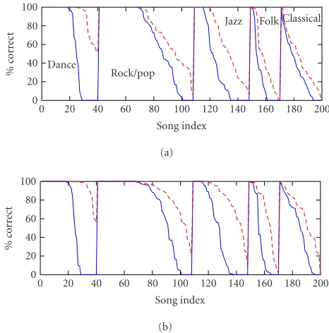
Figure 2shows the results for model one over the whole database graphically whileFigure 3shows the same for model two. These are ordered by style and then performance within the style category. Figure 4 shows the tempo profile for a correctly tracked example using model one; note the close agreement between the hand labelled data and the tracked tempo.
8. DISCUSSION
The algorithms described above have some similar elements but their fundamental operation is quite different: the Rao-Blackwellised model ofSection 5actually bears a significant resemblance to an interacting multiple models system of the type used in radar tracking [33], as many of the stages are actually deterministic. The second model, however, is much
5The clapped signals were often slightly in error themselves.
Dance
Rock/pop
Jazz Folk Classical
0 20 40 60 80 100 120 140 160 180 200 Song index
0 20 40 60 80 100
%c
o
rr
ec
t
(a)
0 20 40 60 80 100 120 140 160 180 200 Song index
0 20 40 60 80 100
%c
o
rr
ec
t
(b)
Figure2: Results on test database for model one. The solid line rep-resents raw performance and the dashed line is performance after acceptable tracking errors have been taken into account. (a) Maxi-mum length correct (% of total). (b) Total percentage correct.
more typically a particle filter with mainly stochastic pro-cesses. Both have many underlying similarities in the model though the inference processes are significantly different.
Thus, the results highlight some interesting compar-isons between these two philosophies. On close examination, model two was better at finding the most likely local path through the data, though this was not necessarily the correct one in the long term. A fundamental weakness of the models is the prior on ck (or equivalently,τk in model two) which
intrinsically prefers higher tempos—doubling a given tempo places more onsets in metrically stronger positions which is deemed more likely by the prior given in (17). Because the stochastic resampling step efficiently selects and boosts high probability regions of the posterior, model two would often pick high tempos to track (150-200bpm) which accounts for the very low “raw” results.
A second problem also occurs in model two: because du-plication of paths through theτ1:kspace is necessary to fully
populate each quantisation hypothesis, fewer distinct paths are kept at each iteration. By comparison, theN-best selec-tion scheme of model one ensures that each particle repre-sents a uniquec1:kset and more paths through the state space
Dance
Rock/pop Jazz Folk Classical
0 20 40 60 80 100 120 140 160 180 200 Song index
0 20 40 60 80 100
%c
o
rr
ec
t
(a)
0 20 40 60 80 100 120 140 160 180 200 Song index
0 20 40 60 80 100
%c
o
rr
ec
t
(b)
Figure3: Results for model two. (a) Maximum length correct (% of total). (b) Total percentage correct.
The remaining lack of performance can be accredited to four causes: the first is tracking at multiple tempo modes— sometimes tracking fails at one mode and settles a few beats later into a second mode. The results only reflect one of these modes. Secondly, stable tracking sometimes occurs at psy-chologically implausible modes (e.g., 1.5 times the correct tempo) which are not included in the results above. The third cause is poor onset detection. Finally, there are also examples in the database which exhibit extreme tempo variation which is never followed.
The result of this is a number of suggestions for improve-ments: firstly, the onset detection is crucial and if the detected onsets are unreliable (especially at the start of an example) it is unlikely that the algorithm will ever be able to track the beat properly. This may suggest an “online” onset detec-tion scheme where the particles propose onsets in the data, rather than the current offline, hard decision system. The other potential scheme for overcoming this would be to pro-pose a salience measure (e.g., [21]) and directly incorporate this into the state evolution process, thus hoping to diff eren-tiate between likely and unlikely beat locations in the data; currently, the Rao-Blackwellised amplitude process has been given weak variances and hence has little effect in the algo-rithm, other than to propose correct phase. The other prob-lems commonly encountered were tempo errors by plausi-ble ratios; Metropolis-Hastings steps [27] to explore other modes of the tempo posterior were tried but have met with little success.
Thus it seems likely that any real further improvement will have to come from music theory incorporated into the algorithm directly, and in a style-specific way—it is unlikely that a beat tracker designed for dance music will work well on choral music! Thus, data expectations and also
antici-Dave Matthews band—best of what’s around (live)
0 10 20 30 40 50
Time (s) 94
96 98 100 102 104 106 108
Te
m
p
o
(B
P
M
)
Hand-labelled tempo Estimated tempo
Figure4: Tempo evolution for a correctly tracked example using model one.
pated tempo evolutions and onset locations would have to be worked into the priors in order to select the correct tempo. This will probably result in an algorithm with many ad-hoc features but, given that musicians have spent the better part of 600 years trying to create music which confounds expec-tation, it is unlikely that a simple, generic model to describe all music will ever be found.
9. CONCLUSIONS
Two algorithms using particle filters for generic beat track-ing across a variety of musical styles are presented. One is based upon the Kalman filter and is close to a multiple hy-pothesis tracker. This performs better than a more stochastic implementation which models tempo as a Brownian motion process. Results with the first model are comparable with the current state of the art [14]. However, the advantage of parti-cle filtering as a framework is that the model and the imple-mentation are separated allowing the easy addition of extra measures to discriminate the correct beat. It is conjectured that further improvement is likely to require music specific knowledge.
ACKNOWLEDGMENTS
REFERENCES
[1] C. Raphael, “A probabilistic expert system for automatic mu-sical accompaniment,”J. Comput. Graph. Statist., vol. 10, no. 3, pp. 486–512, 2001.
[2] F. Gouyon, L. Fabig, and J. Bonada, “Rhythmic expressiveness transformations of audio recordings: swing modifications,” in
Proc. Int. Conference on Digital Audio Effects Workshop, Lon-don, UK, September 2003.
[3] G. Tzanetakis and P. Cook, “Musical genre classification of audio signals,” IEEE Trans. Speech, and Audio Processing, vol. 10, no. 5, pp. 293–302, 2002.
[4] E. D. Scheirer, “About this business of metadata,” in Proc. International Symposium on Music Information Retrieval, pp. 252–254, Paris, France, October 2002.
[5] J. Sepp¨anen, “Tatum grid analysis of musical signals,” in
Proc. IEEE Workshop on Applications of Signal Processing to Au-dio and Acoustics, pp. 131–134, New Paltz, NY, USA, October 2001.
[6] S. W. Hainsworth, Techniques for the automated analysis of musical audio, Ph.D. thesis, Cambridge University Engineer-ing Department, Cambridge, UK, 2004.
[7] E. D. Scheirer, “Tempo and beat analysis of acoustical musical signals,” J. Acoust. Soc. Amer., vol. 103, no. 1, pp. 588–601, 1998.
[8] E. W. Large and M. R. Jones, “The dynamics of attending: How we track time varying events,”Psychological Review, vol. 106, no. 1, pp. 119–159, 1999.
[9] J. Foote and S. Uchihashi, “The beat spectrum: a new ap-proach to rhythm analysis,” inProc. IEEE International Con-ference on Multimedia and Expo, pp. 881–884, Tokyo, Japan, August 2001.
[10] M. Goto, “An audio-based real-time beat tracking system for music with or without drum-sounds,” J. of New Music Re-search, vol. 30, no. 2, pp. 159–171, 2001.
[11] S. Dixon, “Automatic extraction of tempo and beat from ex-pressive performances,”J. of New Music Research, vol. 30, no. 1, pp. 39–58, 2001.
[12] J. Laroche, “Estimating tempo, swing and beat locations in audio recordings,” inProc. IEEE Workshop on Applications of Signal Processing to Audio and Acoustics, pp. 135–138, New Paltz, NY, USA, October 2001.
[13] C. Raphael, “Automated rhythm transcription,” inProc. Inter-national Symposium on Music Information Retrieval, pp. 99– 107, Bloomington, Ind, USA, October 2001.
[14] A. Klapuri, “Musical meter estimation and music transcrip-tion,” inProc. Cambridge Music Processing Colloquium, pp. 40–45, Cambridge University, UK, March 2003.
[15] R. D. Morris and W. A. Sethares, “Beat tracking,” in7th Valencia International Meeting on Bayesian Statistics, Tenerife, Spain, June 2002, personal communication with R. Morris. [16] A. T. Cemgil and B. Kappen, “Monte Carlo methods for
tempo tracking and rhythm quantization,”J. Artificial Intelli-gence Research, vol. 18, no. 1, pp. 45–81, 2003.
[17] J. A. Bilmes, “Timing is of the essence: perceptual and compu-tational techniques for representing, learning and reproduc-ing expressive timreproduc-ing in percussive rhythm,” M.S. thesis, Me-dia Lab, MIT, Cambridge, Mass, USA, 1993.
[18] C. Drake, A. Penel, and E. Bigand, “Tapping in time with me-chanical and expressively performed music,”Music Perception, vol. 18, no. 1, pp. 1–23, 2000.
[19] D.-J. Povel and P. Essens, “Perception of musical patterns,”
Music Perception, vol. 2, no. 4, pp. 411–440, 1985.
[20] H. C. Longuet-Higgins and C. S. Lee, “The perception of mu-sical rhythms,”Perception, vol. 11, no. 2, pp. 115–128, 1982.
[21] R. Parncutt, “A perceptual model of pulse salience and metri-cal accent in musimetri-cal rhythms,”Music Perception, vol. 11, no. 4, pp. 409–464, 1994.
[22] M. J. Steedman, “The perception of musical rhythm and me-tre,”Perception, vol. 6, no. 5, pp. 555–569, 1977.
[23] A. Doucet, S. Godsill, and C. Andrieu, “On sequential Monte Carlo sampling methods for Bayesian filtering,”Statistics and Computing, vol. 10, no. 3, pp. 197–208, 2000.
[24] N. J. Gordon, D. J. Salmond, and A. F. M. Smith, “Novel ap-proach to nonlinear/non-Gaussian Bayesian state estimation,”
IEE Proceedings Part F: Radar and Signal Processing, vol. 140, no. 2, pp. 107–113, 1993.
[25] A. F. M. Smith and A. E. Gelfand, “Bayesian statistics without tears: a sampling-resampling perspective,” Amer. Statist., vol. 46, no. 2, pp. 84–88, 1992.
[26] M. S. Arulampalam, S. Maskell, N. Gordon, and T. Clapp, “A tutorial on particle filters for online nonlinear/non-Gaussian Bayesian tracking,” IEEE Trans. Signal Processing, vol. 50, no. 2, pp. 174–188, 2002.
[27] A. Doucet, N. J. Gordon, and V. Krishnamurthy, “Particle fil-ters for state estimation of jump Markov linear systems,”IEEE Trans. Signal Processing, vol. 49, no. 3, pp. 613–624, 2001. [28] G. Casella and C. P. Robert, “Rao-Blackwellisation of
sam-pling schemes,”Biometrika, vol. 83, no. 1, pp. 81–94, 1996. [29] C. Duxbury, M. Sandler, and M. Davies, “A hybrid approach
to musical note detection,” inProc. 5th Int. Conference on Dig-ital Audio Effects Workshop, pp. 33–38, Hamburg, Germany, September 2002.
[30] S. Abdallah and M. Plumbley, “Unsupervised onset detection: a probabilistic approach using ICA and a hidden Markov clas-sifier,” inProc. Cambridge Music Processing Colloquium, Cam-bridge, UK, March 2003.
[31] S. W. Hainsworth and M. D. Macleod, “Onset detection in musical audio signals,” inProc. International Computer Mu-sic Conference, pp. 163–166, Singapore, September–October 2003.
[32] Y. Bar-Shalom and T. E. Fortmann, Tracking and Data As-sociation, vol. 179 ofMathematics in Science and Engineering, Academic Press, Boston, Mass, USA, 1988.
[33] S. S. Blackman and R. Popoli,Design and Analysis of Modern Tracking Systems, Artech House, Norwood, Mass, USA, 1999. [34] W. R. Gilks, S. Richardson, and D. J. Spiegelhalter, Eds.,
Markov chain Monte Carlo in practice, Chapman & Hall, Lon-don, UK, 1996.
[35] B. Øksendal, Stochastic Differential Equations, Springer-Verlag, New York, NY, USA, 3rd edition, 1992.
[36] M. Orton and A. Marrs, “Incorporation of out-of-sequence measurements in non-linear dynamic systems using particle filters,” Tech. Rep., Cambridge University Engineering De-partment, Cambridge, UK, 2001.
Malcolm D. Macleodwas born in 1953 in Cathcart, Glasgow, Scotland. He received the B.A. degree in 1974, and Ph.D. on dis-crete optimisation of DSP systems in 1979, from the University of Cambridge. From 1978 to 1988 he worked for Cambridge Consultants Ltd, on a wide range of sig-nal processing, electronics, and software research and development projects. From 1988 to 1995 he was a Lecturer in the Signal