On the Optimal Pre-Computation of Window
τ
NAF
for Koblitz Curves
William R. Trost
∗and Guangwu Xu
†Abstract
Koblitz curves have been a nice subject of consideration for both theoretical and practical interests. The window τ-adic algorithm of Solinas (window τNAF) is the most powerful method for computing point multiplication for Koblitz curves. Pre-computation plays an important role in improving the performance of point multi-plication. In this paper, the concept of optimal pre-computation for window τNAF is formulated. In this setting, an optimal pre-computation has some mathematically natural and clean forms, and requires 2w−2−1 point additions and two evaluations
of the Frobenius map τ, where w is the window width. One of the main results of this paper is to construct an optimal pre-computation scheme for each window width
w from 4 to 15 (more than practical needs). These pre-computations can be easily incorporated into implementations of windowτNAF. The ideas in the paper can also be used to construct other suitable pre-computations. This paper also includes a discussion of coefficient sets for window τNAF and the divisibility by powers of τ
through different approaches.
Keywords: Elliptic curve cryptography, window τ-non adjacent form, pre-computation
1
Introduction
One of the most important families of elliptic curves in elliptic curve cryptography (ECC) is the Koblitz curves [10]. A Koblitz curve over F2m is defined by
Ea:y2+xy=x3+ax2 + 1,
∗Department of EE & CS, University of Wisconsin-Milwaukee, Milwaukee, WI 53211, USA; e-mail:
†Department of EE & CS, University of Wisconsin-Milwaukee, Milwaukee, WI 53211, USA; e-mail:
where the parameter a is from {0,1}. On Ea/F2m, the Frobenius map is defined as: for
point (x, y) that is different from the point at infinity
τ(x, y) = (x2, y2),
and for the point at infinity O, τ(O) =O.
Letµ= (−1)1−a. Since τ2(P) + 2P =µτ(P) for allP ∈E
a(F2m),τ can be interpreted
as a complex number defined by τ2−µτ + 2 = 0. One can choose
τ = µ+
√ −7 2 .
Therefore the Euclidean domain Z[τ] =Z+Zτ can be identified as a set of automorphisms of Ea in the sense that
(g+hτ)P =gP +hτ(P).
for every P ∈Ea(F2m).
In ECC, one considers the situation where |Ea(F2m)| is very nearly prime, that is,
|Ea(F2m)| = |Ea(F2)| ·p for some prime p > 2. The main subgroup M of Ea(F2m) is the
subgroup of order p. For δ = τ
m−1
τ−1 , we have the norm Na(δ) = p
1 and δ(P) = O for
P ∈M. The latter yields a useful fact which asserts that for elements ρ and γ in Z[τ], if
ρ≡γ( mod δ), then for every P ∈M,
ρP =γP. (1.1)
The Frobenius map τ is an inexpensive operation as squaring in F2m can be done
efficiently. Based on this, Koblitz [10] proposed a method of computing the point multipli-cation nP by representing n=Pki=0ciτi with ci ∈ {0,1} and evaluatingPki=0ciτi(P).
In [13], Solinas developed a width-wwindowτ-adic method for the efficient computation of nP. The procedure can be briefly described as
1. Reduction. Find some suitableρ=r1+r2τ ∈Z[τ] with |r1|,|r2|being roughly
√
n, such that
ρ≡n (mod δ).
Then by (1.1), computing nP is equivalent to computing ρP.
2. Window τ-NAF. Fix a positive integer w. Denote the coefficient set
Cmin ={c1, c3,· · · , c2w−1−1} (1.2) 1For an element r
0+r1τ ∈Z[τ], its norm isNa(r0+r1τ) = (r0+r1τ)(r0+r1τ¯) = r20+µr0r1+ 2r21.
where cj is an element with the least norm from the odd congruence class j = {c∈
Z[τ] :c≡ j (mod τw)}, (j = 1,3,· · · ,2w−1−1). The width-w τ non-adjacent form
of ρ is
ρ=
l−1
X
i=0
εiuiτi,
where εi ∈ {−1,1} and ui ∈ Cmin ∪ {0} with the properties that in any segment
{uk, uk+1,· · · , uk+w−1} of length w , there is at most one nonzero ui. We denote the
above expression of ρby τNAFw(n).
3. Pre-Computation: Compute Qj = cjP for each j = 1,3,· · · ,2w−1−1. Note that
c1 = 1, so Q1 =P needs no calculation.
4. Computing nP: Evaluate ρP by Horner’s rule, using τNAFw(n) and precomputed
Q1, Q3,· · · , Q2w−1. Discarding the zero coefficients, theτNAFw(n) ofρcan be written
as
ρ=ε0ck0τ k0 +ε
1ck1 | {z }
k1−k0≥w
τk1 +ε
2ck2 | {z } k2−k1≥w
τk2 +· · ·+ε
s−1cks−1τ
ks−1 +ε scks
| {z } ks−ks−1≥w
τks
with εj ∈ {−1,1} and ckj ∈ Cmin. So nP =ρP can be computed through
nP =τk0(τk1−k0(· · ·(τks−ks−1ε
sQjks +εs−1Qjks−1) +· · ·+ε1Qjki1) +ε0Qjk0).
As indicated in [13], for practical values of w, pre-computation requires 2w−2−1 point
additions. The example (Table 1) given in [13] shows how to construct the pre-computation for the case of w= 5, a= 1, i.e.,
Table 1: Pre-computation from [13]
Q3 =τ2P −P Q5 =τ2P +P Q7 =−τ3P −P Q9 =−τ3Q5+P
Q11 =−τ2Q5−P Q13 =−τ2Q5+P Q15=τ4P −P
It can be seen that, in addition to 2w−2−1 = 7 point additions, 7 evaluations of τ are also needed, i.e., we need to compute τ P, τ2P, τ3P, τ4P and τ Q
5, τ2Q5, τ3Q5.
Some improved pre-computations are discussed in [7] where eight cases (i.e., 3 ≤w ≤
Table 2: Pre-computation from [7]
Q3 =τ2P −P Q5 =τ2P +P Q7 =−τ3P −P Q9 =−τ3Q5+P
Q11=−τ2Q5−P Q13=−τ2Q5 +P Q15 =τ2Q5−Q5
Such pre-computation have been used in the discussion of [1].
In [3], Blake, Murty and Xu extended Solinas’s method by allowing a general coefficient set of the form
Cnm ={c1, c3,· · · , c2w−1−1} (1.3)
wherec1 = 1 andcj is an element from the odd congruence classj that satisfiesN(cj)<2w,
for j = 3,· · · ,2w−1 −1. It is easy to see that C
min is a special case of Cnm. It has been
proved in [3] that the algorithm for computing τNAFw(ρ) (Algorithm 4 of [13]) is correct
for the general coefficient sets. In particular, [3] provided a termination proof ofτNAFw(ρ)
for the original setting of Cmin. See also [4].
Examples of efficient pre-computation were given in [3]. For the case w = 5, a = 1, example 3 of [3] greatly improved that of [13] by requiring only two evaluations of τ. The pre-computation is
Table 3: Pre-computation from [3]
Q3 =τ2P −P Q5 =τ P −P Q7 =τ P +P Q9 =τ P +Q3
Q11=τ P +Q5 Q13=τ P +Q7 Q15=τ P +Q9
This pre-computation is actually an optimal one (as explained later).
The purpose of this paper is to systematically study pre-computation for windowτNAF for Koblitz curves. As we shall see later, for eachw >2, a pre-computation requires at least 2w−2 −1 point additions and two evaluations of τ ( except for the simple case of w = 3
where one application of τ is sufficient). We shall call a pre-computation that involves 2w−2−1 point additions and two evaluations ofτ anoptimal pre-computation. One of the
main results of this paper is to show that for each of the cases 4 ≤ w ≤ 15, a = 0,1, an optimal pre-computation exists. These cover all of practical interesting cases2.
A computationally efficient criterion for divisibility of an element g +hτ ∈ Z[τ] by a power of τ is needed in determining a residue modulo τw. This is a useful step for
2As indicated in [13], w >8 is no longer practical, due to the fact that the total cost of using window
forming the coefficient set Cnm for the windowτNAF, hence for the pre-computation. Such
criterion was described by Solinas [13] in terms of Lucas sequences. In this paper, we present a different approach by refining the p-adic argument of Blake, Murty and Xu [4]. This also provides an explanation of the divisibility by a power of τ in the ring Z[τ] from another view point. The generality of the computational procedure for divisibility is also useful in our construction of optimal pre-computations.
The rest of the paper is organized into three sections. The next section discusses the algebraic setup of pre-computations. Section 3 will be devoted to a detailed formulation and description of optimal pre-computations. The last section is the conclusion.
2
The Coefficient Sets for Window
τ
NAF
In our discussion in the previous section, for Koblitz curves, the point multiplication nP
can be turned into a complex multiplication (r1 +r2τ)P for r1, r2 ∈ Z. Efficiency can be
archived by using the window τNAF of r1 +r2τ. In this section, we shall consider the
construction of the coefficient sets for window τNAF. To this end, we need to work with the (algebraic) integer ring Z[τ] ={g+hτ :g, h∈Z}.
Given a positive integerw, the coefficient setCnmfor windowτNAF is the key ingredient
for the pre-computation. Recall that Cnm is constructed by taking one element from each
odd congruence class j modulo τw whose norm is less than 2w, for j = 1,3,· · · ,2w−1−1. For each j = 3,· · · ,2w−1−1, define
Rj ={g+hτ :g+hτ ≡j (mod τw), Na(g+hτ)<2w}.
Assume that an explicit coefficient set is
Cnm ={c1, c3,· · · , c2w−1−1}
where c1 = 1 and cj ∈Rj forj = 3,· · · ,2w−1−1. We can see that in the setting of [3], the
coefficient sets for a window τNAF (or pre-computations) are quite flexible. There are
2w−2−1 Y
k=1
R2k+1
choices of Cnm.
In order to determine the setRj, we need to find suitableg+hτ such thatτw|g−j+hτ.
The problem of divisibility by a power of τ was studied in [13]. Using the Lucas sequence, Solinas proved that there is an integer tw such that
In [4], a p-adic approximation approach was proposed for the problem of divisibility by a power of a zero of a quadratic polynomial of the form X2+kX +p with |k|< p. Here we
give an intuitive and a computational refinement of the argument for the case p = 2 and polynomial f(X) = X2 −µX + 2. Using Hensel’s lifting algorithm [8, 12], starting from
s1 = 0, we can get thenth 2-adic approximation
sn =b12 +b222+· · ·+bn−12n−1
of the 2-adic zero α =
∞ X
k=1
bk2k of f(X) by the following procedure:
Procedure 2.1: The nth 2-adic Approximation
s1 ←0;
for ( i from 1 to n−1 ) do
bi ← f(2sii)µ (mod 2) ; //f(si) is divisible by 2
i.
si+1 ←si+bi2i;
By this procedure, we can easily get:
s2 s3 s4 s5 s6 s7 s8 s9 · · ·
2µ 6µ 6µ 6µ 38µ 38µ 166µ 422µ · · ·
In general, we can get a positive integer qn such that
sn=qnµ. (2.2)
Note that 2|α and 2n|α−sn, so we have
αn|g+hα ⇐⇒ 2n|g+hsn.
This naturally leads to the following argument
τw|g+hτ ⇐⇒ 2w|g+hsw. (2.3)
We will not explain the proof of (2.3) here, as a rigorous proof of the general p-adic case has already been given in [4].
Note that
Na(g+hτ) =g2+µgh+ 2h2 =
3g2
4 +
g
2+µh
2
+h2,
so the requirement Na(g+hτ) <2w forces |g| ≤ b2
w+2 2 √
3 c and |h| ≤ b2
w
2c. With these, we
Procedure 2.2: Generation of Rj
Rj ← ∅;
for ( h from −b2w2c to b2
w
2c ) do
for ( g from −b2w√+22
3 c to b 2√w+22
3 c ) do
if ( (2w|g−j+hs
w) and (g2+µgh+ 2h2 <2w ) )
append (g+hτ) to Rj;
3
Optimal Pre-computations
Once a coefficient set Cnm = {c1, c3,· · · , c2w−1−1} is specified, the pre-computation can be
performed. Given the base pointP, this is the task for computing and storing the 2w−2−1 points
Q3 =c3P, Q5 =c5P, · · · , Q2w−1−1 =c2w−1−1P.
For the sake of convenience, in the rest discussion, we set c1 = 1 and Q1 = P. We also
remark that the pre-computations for the case of w= 3 is very simple and only Q3 needs
to be computed:
Pre-computation for w= 3
a= 0 Q3 =P +τ(P) a= 1 Q3 =P −τ(P)
So we shall be interested in the cases ofw >3 in the rest of the section. Another remark we would like to make is that an efficient pre-computation may be achieved with rearranging the order ofQ1, Q3, Q5,· · · , Q2w−1−1. In the actual computation, we may need to compute
some Qj beforeQk, even though j > k.
Now we begin the setup of optimal pre-computation.
We first observe that there are only two elliptic curve operations involved in the pre-computation, the point addition (include point doubling) and evaluation of τ. As pointed out in [13], for w in the practical range (for w from 3 to 8), each Qj (j ≥3) can be done
by using one point addition operation, plus some evaluations ofτ. The cost of the latter is comparatively less.
Next we argue that, in terms of point addition operation, one operation for each Qj
(j = 3,5,· · · ,2w−1 −1) is necessary. If not, suppose that some Q
j0 is obtained by only
using τ to some previous computed Qk (this should include Q1 = P). This means that
cj0 = τ ec
k. Note that j0 is an odd number, so j0 ≡ 1 (mod τ) (since 2 = τ(µ−τ)).
Therefore
τeck = cj0 ≡j0 (mod τ w)
This implies that there is a u∈Z[τ] such that
τ u= 1.
This is absurd as Na(τ u) = Na(τ)Na(u) = 2Na(u) > 1. Thus point addition operation
must be used in computing Qj ( j ≥3).
Finally, we turn to the other operation, the Frobenius mapτ. Concerning the efficiency of using τ in pre-computation, there has not been a clean argument yet. As mentioned earlier, the example in [13] discussed the case w = 5, a = 1, and 7 evaluations of τ were needed. An improvement for this case was suggested in [7] with 6 evaluations of τ. The other cases discussed in [7] include w = 4 ( with 3 evaluations of τ ) and w = 6 ( with 12 evaluations of τ ). For the casew= 5, a= 1, a more efficient pre-computation scheme was proposed in [3]. This scheme uses only two evaluations of τ, namely τ(P) and τ(τ(P)). The interesting fact is that this is the best one can do. In general, we can argue that under the assumption that 4 ≤ w ≤ 15, and only one point addition is allowed for each
Qj (j = 3,5,· · · ,2w−1 −1), then we need at least two evaluations of τ to finish the
pre-computation. In fact, suppose we have a pre-computation
Qj1 =P, Qj3, Qj5, · · · , Qj2w−1−1.
SinceQj3 is the first term that needs to be computed, it must be of the form ofε1P+ε2τ e(P),
where ε1, ε2 ∈ {−1,1} and e≥1. Assume that we could get the pre-computation done by
using only one evaluation of τ, then this evaluation must be τ(P). So e= 1 and for each
k > 3, we have
Qjk =ε1Qjl+ε2τ(P),
for some l < k and ε1, ε2 ∈ {−1,1}. In terms of the elements in the coefficient set Cnm,
this means that for each k >3, there is anl < k and ε1, ε2 ∈ {−1,1}, such that
cjk =ε1cjl+ε2τ. (3.1)
This has been proved to be impossible by checking all possible sets of Cnm.
Based on these discussions, we define anoptimal pre-computationforQ1, Q3, Q5,· · · , Q2w−1−1
to be a pre-computation satisfying
1. Computation of each of Q3, Q5,· · · , Q2w−1−1 uses only one point addition;
2. The entire pre-computation uses only two special evaluations of τ, namely τ(P) and
τ(τ(P)).
We would like to point out that this formulation of optimal pre-computation is mathe-matically natural and clean. In particular, if an optimal pre-computation for the curve
y2+xy=x3+ 1/
F2m (ie., the parametera= 0) is found, then an optimal pre-computation
for the curve y2 +xy = x3 +x2 + 1/
F2m (ie., the parameter a = 1) can be constructed
Proposition 3.1 Assume that an optimal pre-computation with Qj’s are computed in the following order
Qj1 =P, Qj3, Qj5, · · · , Qj2w−1−1. Then
1. For each k ≥3, there is an l < k and ε1, ε2 ∈ {−1,1} such that
Qjk =ε1Qjl+ε2τ
e(P), (3.2)
with e= 1 or 2.
2. If an optimal pre-computation of the form (3.2) is found for a = 0 (a = 1), then we have an optimal pre-computation Qj1 = P, Qj3, Qj5, · · ·, Qj2w−1−1 for a =
1 (a= 0) with the following form
Qjk =ε1Qjl+ε2(−1)
eτe(P),
Proof.
1. Since Qjk is formed using one addition, it can be either
Qjk =ε1Qjl+ε2Qjd,
for l, d < k, or
Qjk =ε1Qjl+ε2τ
e(P),
for l < k and e= 1 or 2.
Thus we only need to prove the first case is false. Indeed, as cjl and cjd are chosen
from odd congruence classes, and both have smaller norms, representing the relation
Qjk =ε1Qjl+ε2Qjd as
cjkP = (ε1cjl+ε2cjd)P,
we get cjk = (ε1cjl +ε2cjd). This implies that cjk is in an even congruence class.
However, the coefficients must be from odd classes, so this is a contradiction.
2. Leta = 0 and an optimal pre-computation is of the form (3.2). This means thatQj3
must be of the form ε1P +ε2τe(P), and each following Qjk is obtained by adding
ε3τe
0
(P) to some previous one. So Qjk can be written as
Qjk =εP +z1τ(P) +z2τ
2(P), for ε∈ {−1,1} and some z
1, z2 ∈Z. (3.3)
This, together with the fact that τ2 =µτ −2, mean that,
cjk =ε+z1τ +z2τ
2 = (ε−2z
Since cjk ≡jk (mod τ
w), by (2.3) and (2.2), we have
2w|(ε−2z2 −jk) + (z1+µz2)qwµ.
Note that in this case, µ= (−1)1−a =−1, so we have
2w|(ε−2z2−jk) + (z2−z1)qw. (3.4)
Now consider the case of a = 1. In this case, µ = (−1)1−a = 1. So (3.4) can be reorganized as
2w|(ε−2z2 −jk) + (−z1+µz2)qwµ.
Using (2.3) again, we see that τw|(ε−2z
2−jk) + (−z1+µz2)τ, i.e.,
ε−z1τ +z2τ2 ≡jk (mod τw).
Denote c0j
k =ε−z1τ+z2τ
2, since N
1(c0jk) =N0(cjk), so
{1, c0j3, c0j5,· · · , c0j
2w−1−1}
is a coefficient set of window τNAF for the case of a = 1. For the corresponding pre-computation, we let Qjk =c
0
jkP =εP −z1τ(P) +z2τ
2(P). Observe that we only
change the sign of the confident of τ in the expression (3.3), so this pre-computation must satisfy
Qjk =ε1Qjl+ε2(−1)
eτe(P).
The proof of constructing an optimal pre-computation for the case a = 0, from the case a = 1, is analogous.
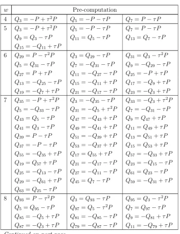
The main result in this section is to show that for w from 4 to 15, there is always an optimal pre-computation for the window τNAF.
Theorem 3.1 For each w from 4to 15, there exists a coefficient Cnm whose corresponding pre-computation can be arranged as
Qj1 =P, Qj3, Qj5, · · · , Qj2w−1−1.
such that for each k >3, there is an l < k and ε1, ε2 ∈ {−1,1}, one has either
Qjk =ε1Qjl+ε2τ(P),
or
Qjk =ε1Qjl +ε2τ
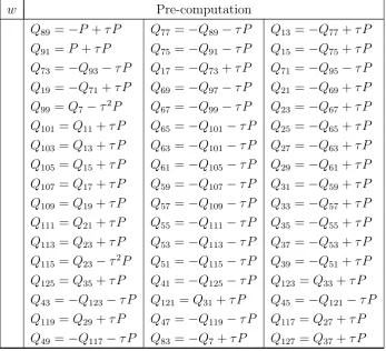
The proof of this result is done by simply displaying all of these optimal pre-computations. We remark that these pre-computations can be easily used in the implementation of window
τNAF.
We will list the pre-computations for the cases of 4≤w≤8. The cases of 9≤w≤ 15 can be found at http://www.cs.uwm.edu/faculty/gxu4uwm/OptPreComp .
By proposition 3.1, we only need to consider the case of a= 0. The case of a = 1 can be obtained by changing the sign of the coefficient of τ in each Qj from the case of a= 0
(note that the sign of coefficient for τ2 remains unchanged) .
Table 4: Pre-Computations for4≤w≤8 and a= 0
w Pre-computation
4 Q3 =−P +τ2P Q5 =−P −τ P Q7 =P −τ P
5 Q3 =−P +τ2P Q5 =−P −τ P Q7 =P −τ P
Q9 =Q3−τ P Q11 =Q5−τ P Q13=Q7−τ P
Q15=−Q11+τ P
6 Q29=P −τ2P Q3 =Q29−τ P Q31=Q3−τ2P
Q5 =Q31−τ P Q7 =−Q31−τ P Q9 =−Q29−τ P
Q27=P +τ P Q11 =−Q27−τ P Q25=−P +τ P
Q13=−Q25−τ P Q15 =−Q11+τ P Q17=−Q9+τ P
Q19=−Q7+τ P Q21 =−Q17−τ P Q23=−Q3+τ P
7 Q35=−P +τ2P Q3 =−Q35−τ P Q33=−Q3+τ2P
Q5 =−Q33−τ P Q31 =−Q5+τ2P Q7 =−Q31−τ P
Q43=Q5−τ P Q47 =−Q43+τ P Q9 =Q47+τ P
Q41=Q3−τ P Q49 =−Q41+τ P Q11=Q49+τ P
Q39=P −τ P Q51 =−Q39+τ P Q13=Q51+τ P
Q37=−P −τ P Q53 =−Q37+τ P Q15=Q53+τ P
Q55=−Q35+τ P Q17 =Q55+τ P Q57=−Q33+τ P
Q19=Q57+τ P Q21 =−Q17−τ P Q23=−Q15−τ P
Q25=−Q13−τ P Q27 =−Q11−τ P Q61=Q23−τ P
Q29=−Q61+τ P Q45 =Q7−τ P Q59=−Q31+τ P
Q63=Q25−τ P
8 Q93=P −τ2P Q3 =Q93−τ P Q95=Q3−τ2P
Q5 =Q95−τ P Q97 =Q5−τ2P Q7 =Q97−τ P
Q85=−Q5+τ P Q81 =−Q85−τ P Q9 =−Q81+τ P
Q87=−Q3+τ P Q79 =−Q87−τ P Q11=−Q79+τ P
Table 4 –Continued from previous page
w Pre-computation
Q89=−P +τ P Q77 =−Q89−τ P Q13=−Q77+τ P
Q91=P +τ P Q75 =−Q91−τ P Q15=−Q75+τ P
Q73=−Q93−τ P Q17 =−Q73+τ P Q71=−Q95−τ P
Q19=−Q71+τ P Q69 =−Q97−τ P Q21=−Q69+τ P
Q99=Q7−τ2P Q67 =−Q99−τ P Q23=−Q67+τ P
Q101 =Q11+τ P Q65 =−Q101−τ P Q25=−Q65+τ P
Q103 =Q13+τ P Q63 =−Q101−τ P Q27=−Q63+τ P
Q105 =Q15+τ P Q61 =−Q105−τ P Q29=−Q61+τ P
Q107 =Q17+τ P Q59 =−Q107−τ P Q31=−Q59+τ P
Q109 =Q19+τ P Q57 =−Q109−τ P Q33=−Q57+τ P
Q111 =Q21+τ P Q55 =−Q111−τ P Q35=−Q55+τ P
Q113 =Q23+τ P Q53 =−Q113−τ P Q37=−Q53+τ P
Q115 =Q23−τ2P Q51 =−Q115−τ P Q39=−Q51+τ P
Q125 =Q35+τ P Q41 =−Q125−τ P Q123 =Q33+τ P
Q43=−Q123−τ P Q121 =Q31+τ P Q45=−Q121−τ P
Q119 =Q29+τ P Q47 =−Q119−τ P Q117 =Q27+τ P
Q49=−Q117−τ P Q83 =−Q7+τ P Q127 =Q37+τ P
Finally, we list an optimal pre-computation forw= 6, a= 1 based on proposition 3.1. Table 5: Pre-Computations for w= 6 and a = 1
w Pre-computation
6 Q29=P −τ2P Q3 =Q29+τ P Q31=Q3−τ2P
Q5 =Q31+τ P Q7 =−Q31+τ P Q9 =−Q29+τ P
Q27=P −τ P Q11=−Q27+τ P Q25=−P −τ P
Q13=−Q25+τ P Q15=−Q11−τ P Q17=−Q9−τ P
Q19=−Q7−τ P Q21=−Q17+τ P Q23=−Q3−τ P
We would like to conclude this section by the following remark.
Remark 3.1 We remark that in some situations, only one evaluation of τ is needed in an optimal pre-computation. Suppose we are choosing the point P = (xP, yP) on the elliptic curve E1/F2m, then in the process of generation or validation, the equation yP2 +xPyP =
x3
of pre-computation. In this case, as τ(P) = (X2
P, yP2) is already available, an optimal pre-computation only requires one evaluation of τ, i.e., τ2P =τ(τ(P)).
4
Conclusion
Koblitz curves are a family of curves with complex multiplication. The complex multiplica-tion fields for curvesE1 :y2+xy=x3+x2+1/F2mand their “twist”E0 :y2+xy=x3+1/F2m
is Q(√−7). The window τNAF algorithm of Solinas is a successful example of exploring the rich mathematical content to design an extremely efficient point multiplication method. This paper presents a systematic study of the pre-computation schemes for τNAF. We de-fine an optimal pre-computation to be a scheme that allows 2w−2−1 point additions and
two evaluations of τ, for any given window width w ≥ 4 (the case of w = 3 is simple and only one evaluation of τ is needed). This is a mathematically natural setup in that once an optimal pre-computation for Ea is produced, an optimal pre-computation for its
twist E1−a can be obtained without any nontrivial computation. We have constructed
op-timal pre-computations of w from 4 to 15. These pre-computations can be incorporated into implementations of window τNAF. The ideas in the paper can be used to construct other suitable pre-computations. In this paper, we also give a criterion for the divisibility by powers of τ in terms of 2-adic approximation. This is useful in our discussion of the coefficient sets of window τNAF and optimal pre-computation, it might also be of some independent interest.
References
[1] D. Aranha, A. Faz-Hern´andez, J. L´opez, Fr. Rodr´ıguez-Henr´ıquez, Faster implementa-tion of scalar multiplicaimplementa-tion on Koblitz curves,LatinCrypt 2012, LNCS7533, 177-193. [2] I. F. Blake, V. K. Murty and G. Xu, Efficient algorithms for Koblitz curves over fields
of characteristic three,Journal of Discrete Algorithms, 3(2005)113-124.
[3] I. Blake, K. Murty and G. Xu, A note on window τ-NAF algorithm, Information Pro-cessing Letters, 95(2005), no. 5, 496-502.
[4] I. F. Blake, V. K. Murty and G. Xu, Nonadjacent radix-τ expansions of integers in Eu-clidean imaginary quadratic number fields,Canadian Journal of Mathematics, 60(2008), 1267-1282.
[6] I. F. Blake, G. Seroussi and N. Smart, Advances in Elliptic Curve Cryptography, Cam-bridge University Press, 2005.
[7] D. Hankerson, A. Menezes and S. Vanstone, Guide to Elliptic Curve Cryptography,
Springer-Verlag, New York, 2004.
[8] N. Koblitz, p-adic Numbers, p-adic Analysis, and Zeta-Functions,Springer, 1996. [9] N. Koblitz, Elliptic curve cryptosystems, Mathematics of Computation,48 (1987)
203-209.
[10] N. Koblitz, CM-curves with good cryptographic properties, Advances in Cryptology-CRYPTO ’91, LNCS 576, 1992, 279-287.
[11] N. Koblitz, An elliptic curves implementation of the finite field digital signature algo-rithm,Advances in Cryptology-CRYPTO ’98, LNCS 1462, 327-337.
[12] M. R. Murty, Introduction to p-adic Analytic Number Theory,Amer Math. Soc., 2002. [13] J. Solinas, Efficient arithmetic on Koblitz curves, Designs, Codes and Cryptography,
19 (2000), 195-249.
![Table 1: Pre-computation from [13]](https://thumb-us.123doks.com/thumbv2/123dok_us/7908940.1313250/3.595.99.505.541.579/table-pre-computation-from.webp)
![Table 3: Pre-computation from [3]](https://thumb-us.123doks.com/thumbv2/123dok_us/7908940.1313250/4.595.100.514.140.176/table-pre-computation-from.webp)