Hardware-in-the-loop implementation for an active heave compensated drawworks

(1)

Cent. Eur. J. Eng. • 2(2) • 2011 • 201-211 DOI: 10.2478/s13531-011-0062-1

Central European Journal of Engineering

Hardware-in-the-loop implementation for an active

heave compensated drawworks

Research article

Sanin Muraspahic1_{, Peter Gu}1_{, Lawk Farji}1_{, Yousef Iskandarani}1_{, Peng Shi}2,3_{, Hamid Reza Karimi}1∗

1 Department of Engineering, Faculty of Engineering and Science, University of Agder, N-4898 Grimstad, Norway

2 Department of Computing and Mathematical Sciences, University of Glamorgan, Pontypridd, CF37 1DL, UK.

3 School of Engineering and Science, Victoria University, Melbourne, Vic 8001, Australia

Received 24 November 2011; accepted 24 January 2012

Abstract: This paper presents the setup and running of a hardware-in-loop (HIL) simulation for an active heave compensated (AHC) draw-works. A simulation model of the draw-works is executed on a PC to simulate the AHC draw-works with a physical PLC. The PLC (ET200S) is configured with a controller architecture that regulates the motor angular displacement and velocity through actuation of the servo valves. Furthermore, a graphical user interface is developed for operation of the AHC system. The HIL test allowed tuning of the physical controller in terms of heave stabilization and positioning. The conclusion after the testing is a PLC which is ready for operation without necessitating the use a physical prototype of the process.

Keywords: Active heave compensation (AHC) • Draw-works • Hardware-in-the-loop (HIL) • Hoisting rig • Programmable logic controller (PLC)

1. Introduction

HIL simulation was proposed in the early 1990’s as a cost and time saving tool for developing electronic and mecha-nical components [1]. Since then, the application of this strategy for developing embedded systems has become common in several fields. Recent examples include the development of a control system for automatic steering control for an automobile by H. Jamaluddin [2]. Allegre et al. proposed a novel subway design using super capacitors as the main energy source [3]. An HIL test of this design was conducted for experimental validations. Another work

∗_{E-mail: [email protected]}

by Rankin and Jiang used HIL testing to verify the func-tionality of safety control systems within nuclear power plants [4]. Recently, a portable HIL device has also been developed for testing engine control software by Palladino et al. [5].

(2)

Hardware-in-the-loop implementation for an active heave compensated drawworks

1

that regulates the motor angular displacement and velocity through actuation of the servo valves. Furthermore, a graphical user interface is developed for operation of the AHC system. The HIL test allowed tuning of the physical controller in terms of heave stabilization and positioning. The conclusion after the testing is a PLC which is ready for operation without necessitating the use a physical prototype of the

Active heave compensation (AHC), draw-works, hoisting rig, programmable logic

simulation was proposed in the early 1990‘s as a cost and time saving tool for developing electronic and mechanical Since then, the application of this strategy for developing embedded systems has become common in several fields. Recent examples include the development of a control system for automatic steering control for an automobile by H. Jamaluddin [2]. Allegre et al. proposed a novel subway design using super capacitors as the main energy source [3]. An HIL test of this design was conducted for experimental validations. used HIL testing to verify the functionality of safety control systems within nuclear

Muraspahic is with the Department of Engineering, Faculty of Engineering and Science, University of Agder, N-4898 Grimstad, Norway

(e-P. Gu is with the Department of Engineering, Faculty of Engineering and Grimstad, Norway (e-mail:

Farjii is with the Department of Engineering, Faculty of Engineering and Science, University of Agder, N-4898 Grimstad, Norway (e-mail:

Iskandarani is with the Department of Engineering, Faculty of Engineering and Science, University of Agder, N-4898 Grimstad, Norway

(e-P. Shi is with the Department of Computing and Mathematical Sciences, University of Glamorgan, Pontypridd, CF37 1DL, UK. He is also with the School of Engineering and Science, Victoria University, Melbourne, Vic

H.R. Karimi is with the Department of Engineering, Faculty of Engineering and Science, University of Agder, N-4898 Grimstad, Norway

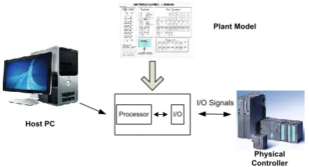
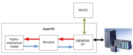
(e-parameters of the model. The principle of HIL is illustrated in Fig.1. Sometimes it may be essential to include physical sensors and actuators in the loop along with the controller. This is so actuator lag and sensor noise can be taken into account. This was done by N.R Gans et al. in the testing of their unmanned air vehicle [6].

Host PC Physical Controller I/O Signals Processor I/O Plant Model

Fig. 1 Principle of HIL simulation.

The advantage for using HIL simulation in developing an embedded system is to be able to tune the controller before its implementation with a physical plant. Furthermore, there may be safety and performance improvements by being able to test various operational scenarios with great flexibility. These could be extreme or failure scenarios which would be potentially dangerous if performed with a physical plant. All in all, HIL testing is a time and cost saving industrial IT tool.

In this case, a simulation model of an active heave compensated draw-works operating on a hoisting rig is to be tested and tuned using HIL simulation. The novelty pertains to utilizing HIL simulation methodology to accelerate the development of active heave compensation systems. So far, to the best of our knowledge, no results are reported with this problem, although similar applications such as the HIL simulation of a fault tolerant system by Karpenko and Sepehri [7] and HIL simulation of a small UAV Helicopter have been done by Guowei et al. [8].

The ground work in this paper was laid by Gu et al. [9] where a SimulationX model of the draw-works and hoisting rig

Figure 1. Principle of HIL simulation.

its implementation with a physical plant. Furthermore, there may be safety and performance improvements by being able to test various operational scenarios with great flexibility. These could be extreme or failure scenarios which would be potentially dangerous if performed with a physical plant. All in all, HIL testing is a time and cost saving industrial IT tool.

In this case, a simulation model of an active heave com-pensated draw-works operating on a hoisting rig is to be tested and tuned using HIL simulation. The novelty per-tains to utilizing HIL simulation methodology to accelerate the development of active heave compensation systems. So far, to the best of our knowledge, no results are reported with this problem, although similar applications such as the HIL simulation of a fault tolerant system by Karpenko and Sepehri [7] and HIL simulation of a small UAV Helicopter have been done by Cai et al. [8].

The ground work in this paper was laid by Gu et al. [9] where aSimulationXmodel of the draw-works and hoisting rig were modeled. All model parameters are explained in their paper.

Motivated by the above discussions, in this paper, we aim to set up the physical controller with the simulation model for an HIL simulation. Also, the goal is to tune and verify the controller for operation during two load cases: the first case is the vertical position stabilization and the second one is the lowering of 5 m to the seabed. In addition, the wire force and drum torque must not exceed design limits. The heave compensation must yield no more than±5 cm of vertical movement for the payload while subject to a sinusoidal wave with an amplitude of 1 m and frequency of 0,1 Hz. This is included in the simulation model by Gu et al [9]. The landing of the payload onto the seabed must occur smoothly with no significant impact forces, yet the lowering should happen within a reasonable time frame.

A control system utilizing feedback signals from the plat-form and draw-works motor needs to be configured. The sensors in this case are thought to be ideal. The actual

control components to be used are two servo valves and a variable displacement motor of two hydraulic power units. This control system does the actual heave compensation and motion control.

To facilitate a HIL simulation a host computer must be set up that allows communication with a physical controller. In this way the controller can interact with the draw-works model.

A PLC is to be used as the physical controller regulating the draw-works model. It needs to be set up for sending and receiving signals from the host PC. It must also have the chosen controller algorithm implemented.

The active heave compensation system must have a graph-ical user interface (GUI) for practgraph-ical operation and obser-vation of the AHC process. In short terms the objectives are to establish communication between physical controller and the draw-works model on the host PC, establish com-munication between the PLC and the GUI, implement a cascade controller on the PLC, and use the GUI to operate the AHC system.

Typically, AHC systems are able to adapt to varying wave conditions and are accurate to about 95% of the desired set point. Korde proposed an active heave compensator and feedback controller to exploit the wide frequency range [10]. Also, in [11], an active heave compensation system is exploited to stabilize the heave platform from the min-ing ship in the irregular wave and a novel active heave compensation system based on dynamic vibration absorber was proposed for deep-sea mining. It was shown that if an un-damped spring-mass system is coupled with a second oscillating system being excited by a sinusoidal external force, then there must exists an excitation frequency at which the second mass will remain stationary for any mag-nitude of excitation. Other recent work on AHC systems include Neupert et al. in [12], who presented a combination of trajectory tracking disturbance decoupling controller and a prediction algorithm for an AHC system. In [13], Li and Liu proposed three-degree-of-freedom dynamic models of an AHC system subject to a sinusoidal wave.

2. Setup for co-simulation

2.1. Industrial IT

The industrial IT part of this work included setting up the communication between the hardware controller and the PC host where the hydro-mechanical model is located. This allows the controller to interact with the model. Con-figuration of the intended control algorithm on the PLC is also completed. Both of these objectives were done in

SIEMENSSTEP7 and downloaded to the PLC.

(3)

S. Muraspahic, P. Gu, L. Farji, Y. Iskandarani, P. Shi, H.R. Karimi

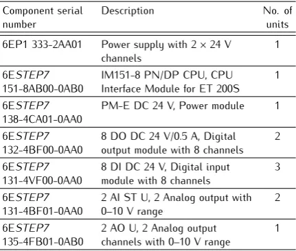
Table 1. Example setup of 3 addresses defined as inputs and 3 as outputs.

Component serial

number Description No. ofunits 6EP1 333-2AA01 Power supply with 2×24 V

channels 1

6ESTEP7

151-8AB00-0AB0 IM151-8 PN/DP CPU, CPUInterface Module for ET 200S 1 6ESTEP7

138-4CA01-0AA0 PM-E DC 24 V, Power module 1 6ESTEP7

132-4BF00-0AA0 8 DO DC 24 V/0.5 A, Digitaloutput module with 8 channels 2 6ESTEP7

131-4VF00-0AA0 8 DI DC 24 V, Digital inputmodule with 8 channels 3 6ESTEP7

131-4BF01-0AA0 2 AI ST U, 2 Analog output with0–10 V range 2 6ESTEP7

135-4FB01-0AB0 2 AO U, 2 Analog outputchannels with 0–10 V range 1

2.2. Communication

SIEMENS ET 200S which is the used PLC controller will be reviewed in this work. ET200S has interface module with integrated PROFINET which uses TCP/IP standards and runs in real-time. However, SIEMENS ET 200S CPU was the only essential component whenever doing Hard-ware in Loop setup. In this paper a setup is designed and constructed in order to facilitate the process of un-derstanding the HIL of the AHC model. In this setup the following components are presented and described as shown in Table1.

The PLC interacts then with the host through an industrial Ethernet standard. The industrial Ethernet standard offer many value propositions added to the simplicity when es-tablishing the connection between PC to the PLC. Siemens STEP7 will be the Ethernet connector to the PLC. There the programmer can store different programs and applica-tions and download them to the PLC. Moreover, it can use different set of languages (STL, FBD, and Ladder) but in this case most programs are implemented as Ladder. TCP/IP is a reliable form of ethernet communication. It uses acknowledgements to confirm that the packets arrive where they are supposing to establish TCP/IP communication between the client and the server is often referred to as a three-way handshake:

• SYN: The client sends a connection request to the server.

• SYN-ACK: The server accepts the request.

• ACK: The client verifies that it has received the acceptance.

Figure 2. Communication fundamentals using TCP/IP protocol.

Figure 3. The hardware setup showing the used SIEMENS ET 200S and peripheral components/accessories.

After the three-way handshake, seen in Fig. 2, packets of information can be sent between the client and the server until one of them sends a FIN package to terminate connection. The three-way handshake is only done when connection is established and will therefore not reduce the performance for the HIL simulation.

The downside by using TCP/IP is that it is not determin-istic. There is no guarantee when the packets will arrive, only that they will arrive and in the correct order. For that reason the latency between each packet of data can vary and cause problems for real-time communication.

The hardware setup as shown in Fig.3consist of the as-sembly of the chosen PLC components as presented in

Table1whereby the assembled components are mounted

(4)

Figure 4. Co-simulation betweenSTEP7andSimulationXthroughMatlab Simulink.

is integrated with switches, LEDs, a voltmeter and poten-tiometer enabling the operator of the plant to access the simulation with an actual signal. It is very important to wire the power module to avoid the failure of the PLC, the hardware setup provides the operator with the feeling of operating an actual process, though it is a simulation. First, communication between the PLC and the host PC must be established. This was done through a hardware configuration on the host PC. The modules and MAC ad-dress for the PLC must be correctly set. Completing this procedure allows communication between the PLC and

SIEMENSSTEP7 on the host PC.

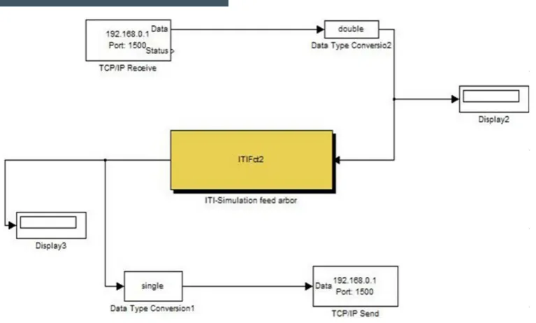
For the PLC to control theSimulationXmodel, communica-tion must be set up internally in the host PC between PLC andSimulationX. This is done through MatlabSimulink using a toolbox called the Instrument Control Toolbox. The setup inSimulink using a simplified model can be seen in Fig. 4. This will be set up for the full model in the HIL chapter. The data that is incoming from the PLC is single (32-bit), which needs to be converted to a double (64-bit) for SimulationX to receive and the opposite for data coming out ofSimulationX.

The data which is being sent from the PLC is received through theTCP/IP receiveblock and sent to theITIFct2

block which is the connection to the TCP/IP block in

SimulationX. The output data fromSimulationX is further sent to theTCP/IP Sendblock which is received by the PLC. For the PLC to send and receive data, a function block calledFB300is used. This block contains the main parameters for communicating with the host PC. In the FB300 block one can set the desiredTSENDandTREC

Table 2. Example setup of 3 addresses defined as inputs and 3 as outputs.

Input Output

“data”.input1 (DBX0.0) “data”.output1 (DBX.12.0) “data”.input2 (DBX4.0) “data”.output2 (DBX16.0) “data”.input3 (DBX8.0) “data”.output3 (DBX.20.0)

signals. Since 4 bytes equals 1 REAL, theTSENDneeds to go from 0.0 to 12.0 bytes andTREC from 12.0 bytes to 20.0. An example of 3 inputs and 3 outputs is shown in Table2.

For the graphical user interface to be able to send data to the PLC it also needs to communicate withSTEP7. To do this the PG/PC (Ethernet) interface must be correctly set, this is done inSTEP7. Furthermore, tags must be set equivalent to the memory addresses. These addresses are the ones that send and receive data fromSimulationX. Completing this will allow operation and observation of the model process in the GUI. Values sent from the GUI to the PLC are received in DB120. From there they are sent to the blocks that use these values. DB121 is used to mirror the values sent to the PLC such as the set point and controller parameters. This allows the operator to observe the set values.

For controlling the draw-works in load case 1 and 2 a cascaded controller was used. The outer controller is a P-controller while the inner controller is a PI-controller. The main reason for using this setup is that the control job is twofold: one is to heave compensate, the other is to lower the payload 5 m. Combining these two load cases

(5)

4 difficult for a single controller feedback system. Therefore, a cascaded controller is selected.

The outer controller is used for positioning the payload. Therefore, its set point is in motor angular displacement. The process variable of the outer loop is the angular displacement of the motor. The output of the outer controller is added with the inner loop set point.

PI Drawworks and Hoisting Rig Model P + -+ -ϴ ϴ 1/s Motor angular velocity sensor Relative valve stroke (Rel) SP1 SP2 + PI Drawworks and Hoisting Rig Model P + -+ -ϴ ϴ 1/s Motor angular velocity sensor Relative valve stroke (Rel) SP1 SP2 +

Fig. 5 Cascade control architecture for the draw-works.

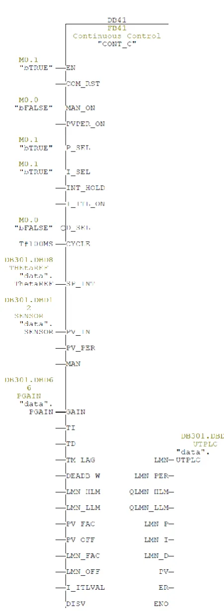
The initial controller concept as shown in Fig. 5 was the cascaded P-PI. To implement this controller two function blocks (FC1 and FC2) were made each representing a controller using TCONT.

Output 1

Outer

P-controller ADD_R Inner PID controller Output 2 Process varibale 2 Setpoint 2 Setpoint 1 Process varibale 1

Fig. 6 Setup of cascade controller in PLC

Both are stored in the OB35 block with an ADDR between them. This is to sum the output of the outer controller with the set point of the inner one. The concept of the setup of the cascade controller in the PLC is shown in Fig. 6. The last network in OB35 works as an enabler to activate the TSEND

function in the communication block FB300.

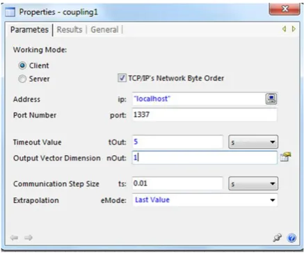
For sending the signals from the hydro-mechanical model which is simulated in SimulationX, a coupling block is introduced which sends the desired signals to the PLC to be regulated through an input vector. The coupling also receives signals from the PLC (regulated signals) which is used to regulate the hydro-mechanical plant. Fig. 7 shows a coupling block from SimulationX.

the more data is being sent since it is a smaller time interval. The bigger the step size the less data will be sent. This means that it almost works as a low pass filter which filters high frequency signal before it sends them to the PLC for regulation.

Fig. 8 Coupling properties C.Operating System

The operating system is the intermediary between hardware and running applications. In order to execute processes and give access to the different hardware, the operating system uses different kinds of scheduling algorithms. Scheduling is necessary because the amount of CPU time is finite and the CPU is not able to execute every task at the same time.

If one process gets higher priority, another process gets lower priority. It is therefore important for the operating system to control these scheduling algorithms in order to optimize the system for a specific task or program.

The different tasks can have three different states:

• Ready: Ready to run in a physical core

• Running: Currently running in the physical core • Blocked/Waiting: Waiting for an external input

There are several different scheduling algorithms for different computer systems, like for example Priority Scheduling, Shortest Job First, Lottery Scheduling and Real-Time Scheduling. Depending on the scheduling algorithm

Figure 5. Cascade control architecture for the draw-works.

Figure 6. Setup of cascade controller in PLC.

could prove difficult for a single controller feedback system. Therefore, a cascaded controller is selected.

The outer controller is used for positioning the payload. Therefore, its set point is in motor angular displacement. The process variable of the outer loop is the angular dis-placement of the motor. The output of the outer controller is added with the inner loop set point.

The initial controller concept as shown in Fig.5was the cascaded P-PI. To implement this controller two function blocks (FC1 and FC2) were made each representing a

controller using TCONT. Both are stored in the OB35

block with an ADDR between them. This is to sum the

output of the outer controller with the set point of the inner one. The concept of the setup of the cascade controller in the PLC is shown in Fig.6. The last network in OB35 works as an enabler to activate theTSENDfunction in the communication block FB300.

For sending the signals from the hydro-mechanical model which is simulated in SimulationX, a coupling block is introduced which sends the desired signals to the PLC to be regulated through an input vector. The coupling also receives signals from the PLC (regulated signals) which is

Figure 7. Coupling block.

Figure 8. Coupling properties.

used to regulate the hydro-mechanical plant. Fig.7shows a coupling block fromSimulationX.

Within the coupling block one can specify the desired port-number, the output vector dimension and most import of all the communication step size. This value shows how much dataSimulationX is sending to the PLC. The smaller the step size the more data is being sent since it is a smaller time interval. The bigger the step size the less data will be sent. This means that it almost works as a low pass filter which filters high frequency signal before it sends them to the PLC for regulation.

2.3. C. Operating System

The operating system is the intermediary between hard-ware and running applications. In order to execute pro-cesses and give access to the different hardware, the oper-ating system uses different kinds of scheduling algorithms. Scheduling is necessary because the amount of CPU time is finite and the CPU is not able to execute every task at the same time.

If one process gets higher priority, another process gets lower priority. It is therefore important for the operating system to control these scheduling algorithms in order to optimize the system for a specific task or program. The different tasks can have three different states:

•Ready: Ready to run in a physical core.

•Running: Currently running in the physical core.

•Blocked/Waiting: Waiting for an external input.

(6)

Figure 9. A hardware-in-the-loop configuration.

Scheduling. Depending on the scheduling algorithm each core in the CPU will generally execute the process with the highest priority that is ready for execution.

By including a HIL test into the commissioning procedure, or at an earlier stage, the design can be tested see if the predicted properties are correct. The engineering companies can save time and money if miscalculations and design flaws are discovered at an earlier stage.

Some tests can be too hazardous for personnel or equip-ment to carry out on the real equipequip-ment. HIL testing can simulate the system responses at critical areas and even above the designed specifications without risking personnel or equipment.

Some desired tests are simply not feasible. For a heave compensator this might be having the desired wave height, speed and length at the desired test time or for example system failure in parts of the system. These scenarios can be carried out in a HIL simulation and tested thoroughly. On a normal operating system such as Linux and Windows the latencies depends on the amount of processes running on the system. A real-time system has a predictable response time and the process should be deterministic. It will typically be a system connected to some kind of external device. CD players, patient monitoring systems and autopilot in an aircraft are all hard real-time systems. A real-time system can generally be divided into two groups:

• Soft real-time system (SRT): Missing an occasional deadline is tolerable. The average process will be executed at deadline.

• Hard real-time system (HRT): Absolute deadlines must be met. The system will stop if the deadline is not met.

Real-time operating systems should meet timing require-ments for the processes they control. Neither Linux nor Windows are real-time operating systems. With Linux the computer gets good overall performance, it utilizes the computer process power in an efficient way, but for sys-tems which require very low response time, or deterministic timing, the standard Linux is not good enough.

5 each core in the CPU will generally execute the process with the highest priority that is ready for execution.

By including a HIL test into the commissioning procedure, or at an earlier stage, the design can be tested see if the predicted properties are correct. The engineering companies can save time and money if miscalculations and design flaws are discovered at an earlier stage.

Some tests can be too hazardous for personnel or equipment to carry out on the real equipment. HIL testing can simulate the system responses at critical areas and even above the designed specifications without risking personnel or equipment.

Some desired tests are simply not feasible. For a heave compensator this might be having the desired wave height, speed and length at the desired test time or for example system failure in parts of the system. These scenarios can be carried out in a HIL simulation and tested thoroughly.

Fig. 9 A hardware-in-the-loop configuration.

On a normal operating system such as Linux and Windows the latencies depends on the amount of processes running on the system. A real-time system has a predictable response time and the process should be deterministic. It will typically be a system connected to some kind of external device. CD players, patient monitoring systems and autopilot in an aircraft are all hard real-time systems.

A real-time system can generally be divided into two groups:

 Soft real-time system (SRT): Missing an occasional deadline is tolerable. The average process will be executed at deadline.

 Hard real-time system (HRT): Absolute deadlines must be met. The system will stop if the deadline is not met. Real-time operating systems should meet timing requirements for the processes they control. Neither Linux nor Windows are real-time operating systems. With Linux the computer gets good overall performance, it utilizes the computer process power in an efficient way, but for systems which require very low response time, or deterministic timing, the standard Linux is not good enough.

Linux can be made into a real-time operating system by adding a real-time kernel. The kernel is the central component of the Linux system; it is the bridge between the applications and the hardware. Linux is better for real-time systems than Windows because it is possible to access the low level programming in the operating system.

Fig. 10 The OB35 continuous block as used in STEP7.

Figure 10. The OB35 continuous block as used inSTEP7.

(7)

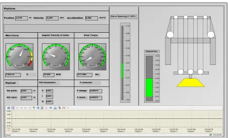
Figure 11. Graphical user interface for the AHC system.

Linux can be made into a real-time operating system by adding a real-time kernel. The kernel is the central com-ponent of the Linux system; it is the bridge between the applications and the hardware. Linux is better for real-time systems than Windows because it is possible to access the low level programming in the operating system.

2.4. Graphical User Interface

The graphical user interface was developed with the WinCC SCADA (Supervisory control data acquisition). This soft-ware is produced by SIEMENS and was used for control and surveillance of industrial processes. WinCC works as a Human Machine Interface (HMI) which connects the operator to the PLC and allows him to change certain values for different types of applications for the AHC of the draw-works.

The final GUI allows adjusting of the payload lowering distance and controller parameters. It also allows obser-vation of important values such as the wire force, drum torque, motor velocity, payload position, platform motion, and valve opening of the servo valves. The GUI can be seen in Fig.11. The trend graph in the bottom half of the figure shows the payload position.

Communication between the PLC and host PC has been established. This means the PLC is enabled for sending

and receiving signals from theSimulationX model. This has also been achieved between the PLC and WinCC GUI. The cascade P-PI regulator has been implemented in the PLC. A WinCC graphical user interface has been developed.

2.5. Hardware in the loop

In this paper, the HIL simulation was ready to be run after the main elements required for such a test were developed:

• Hydro-mechanical simulation model.

• PLC configured with a control algorithm.

• Communication between PLC and a Host PC.

The goal is to tune the PLC for optimal control in load case 1 and 2. The end result should satisfy the requirements of the load cases as well as staying within the limits the hydro mechanical system is dimensioned for.

(8)

Figure 12. HIL setup for active heave compensation of drawworks.

The whole system for sending and receiving signals through Simulink is shown in Fig.13. There are a total of 14 out-puts and 2 inout-puts. Some outout-puts like the Drum Torque which does not have a sensor, can be calculated out of the wire force times the arm in a different operation block in the PLC. The addresses for storing the I/O’s is in DB301.

2.6. Tuning

A manual method of tuning was employed in an attempt to quickly and roughly get within the requirements of±5 cm. Also, Gu et al. [9] have already determined some suitable values which served as a good starting point for manual tuning. Therefore, an optimal tuning approach would yield the best results such as metaheuristics by Fleming and Purshouse [14]. The following guidelines were followed while tuning manually:

• KIandKDvalues set to zero.

• KP should be set to half of the value for a ¼

ampli-tude decay type response.

• IncreaseKIuntil any offset is correct in sufficient

time for the process. Too much increment will cause instability.

• IncreaseKD if required, until the loop reaches

ref-erence after load disturbance acceptably. Too much KDwill cause excessive response and overshoot.

Manual tuning is an iterative process. Starting with only the P-parameter at a value of 0.001, each parameter is tuned until a desirable response is found. Results with P = 0.001 and the rest turned off is used as a reference. It was noticed that having the gain over 0.001 will yield an increased overshoot, but better steady state error. The motor’s actual velocity follows the reference, but oscillates a lot. This is not desirable because the valves will wear out very quickly. TheP-parameter is left at 0.001, while theI- andD-parameters are investigated.

A high I-parameter might be causing instability which makes the payload position drift down to the seabed. Low-ering the value showed better stability with the steady

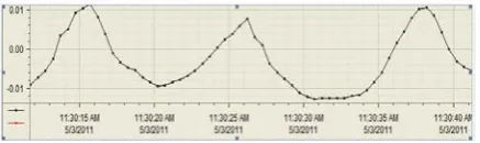
state error being quite small. The point at which theI -parameter started giving worse results for SSE is around 0.031. TheI-parameter seems to have the most effect when it comes to drastically reducing the steady state error. This is however, only if it is within a small range of values. The payload position moves with a range of about 1.1 cm about the equilibrium point, see Fig.15. The actual motor velocity follows the reference velocity and the valve stroke is within an acceptable range. By keeping theI-parameter at 0.031 and increasing or decreasing the gain yield more overshoot, so the P-parameter seems to be optimal at 0.001.

Thus, the gain value of 0.001 and integrator value of 0.031 are kept, while the remainingD-parameter is investigated. Using different values for theD-parameter gave no visible differences from the results with theP- andI-parameters. The conclusion is therefore that theD-parameter is not needed for this application.

3. System verification

Now that the optimal parameters have been found for the outer P-controller and inner PI-controller for load case 1 and 2, the system needs a final verification for its range of operation. This range is the lowering from 0–5 meters. The control system must be able to position the payload optimally in this range, as well as compensate for heave motion. The verification is done by running the AHC with the set point at 0 and increasing with increments of 1 up to the set point is at 5. The results of this verification are seen below for the two load cases: Load case 1: for verification of load case 1 which was to stabilize the position of draw works, the set point was set to 0 m. Fig.16shows that the draw works is heave compensated for wave motion with an oscillation of ± 1 cm.

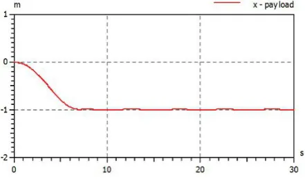
Load case 2: for verification of load case 2 which was to lower the payload to seabed (0–5 m) as smoothly as pos-sible. Figures17–21show the different sets of operations starting at point 0 and increasing with increments of 1. All of the operations had oscillations of ± 1 cm.

4. Conclusion

The industrial IT systematic approach for implementing the HIL for the active heave compensated draw-works model was presented. The extracted AHC model was used to tune the controller for optimal parameters in order to provide the best operational performance during load case 1 and 2. The payload motion was reduced from ± 1 m to ca. ± 1 cm with the activation of the heave compensation. Lowering of the payload was tuned to ca. 10 s with no overshoot

(9)

Figure 13. Communication between PLC and model throughSimulink.

Figure 14. Payload position for load case 1, with inner loopP= 0.001,I= 0.031,D= 0.

meaning a gentle landing. Furthermore, a verification of the system for is done for the range of 0–5 m with increments of 1 m. The results showed the AHC excellent correlation between the controller parameters and the system outputs for this range. Future work will be focused on controller

Figure 15. Payload vertical position during load case 2.

(10)

Figure 16. Set point was set to 0 m and movement shows an oscil-lation of ± 1 cm.

Figure 17. Set point was set to 1 m. Rise time of ca. 3.5 s with no overshoot. Oscillation of ± 1 cm.

Figure 18. Set point was set to 2 m. Rise time of ca. 4 s with no overshoot. Oscillation of ± 1 cm.

Acknowledgments

The authors would like to direct a special thanks to Pro-fessor Geir Hovland for his kind assistance in providing us with the needed hardware, literature and the operation instruction. Further thanks to the technical staff at the

Figure 19. Set point was set to 3 m. Rise time of ca. 5 s with no overshoot, Oscillation of ± 1 cm.

Figure 20. Set point was set to 4 m. Rise time of ca. 5.5 s with no overshoot. Oscillation of ± 1 cm.

Figure 21. Set point was set to 5 m. Rise time of ca. 6 s with no overshoot. Oscillation of ± 1 cm.

Mechatronics laboratory of the University of Agder for the dedication and the enthusiasm which helped and motivate us to reach the project goals.

(11)

References

[1] Hanselmann H., Hardware-in-the loop simulation as a standard approach for development, customization, and production test of ECU’s in 1993 Int. Pacific Conf. On Automotive Engineering

[2] Ping E.P., Hudha K., Jamaluddin H.. Hardware-in-the-loop simulation of automatic steering control for lanekeeping manoeuvre: outer-loop and inner-loop control design, Int. J. Vehicle Safety, Vol. 5, No. 1, 2010, pp. 35–59

[3] Rankin D.J., Jiang J., A Hardware-in-the-loop simu-lation platform for the verification of safety control systems, IEEE Trans. on Nuclear Science, Vol 58, No. 2, April 2011, pp. 468–478

[4] Allegre A.L., Bouscayrol A., Verhille J.N., Delarue P., et al., Reduced-Scale-Power Hardware-in-the-loop sim-ulation of an innovative subway, IEEE Trans. on Indus-trial Electronics, Vol. 57, No. 4, April 2010, pp. 1175– 1185

[5] Palladino A., Fiengo G., Lanzo D., A portable hardware-in-the-loop (HIL) device for automotive di-agnostic control systems, ISA Transactions, in press, corrected proof, November 2011

[6] Gans N.R., Dixon W.E., Lind R., Kurdila A., A hardware in the loop simulation platform for vision-based control of unmanned air vehicles, Mechatronics, Vol. 19, No. 7, October 2009, pp. 1043–1056

[7] Karpenko M., Sepehri N., Hardware-in-the-loop sim-ulator for research on fault tolerant control of

elec-trohydraulic actuators in a flight control application, Mechatronics, 19(7), October 2009, pp. 1067–1077 [8] Cai G., Chen B.M., Lee T.H., Dong M., Design and

implementation of a hardware-in-the-loop simulation system for small-scale UAV helicopters, Mechatronics, 19(7), October 2009, pp. 1057–1066

[9] Gu P., Walid A.A., Iskandarani Y., Karimi H.R., Model-ing, simulation and design optimization of a hoisting rig active heave compensation system, International Journal of Machine Learning and Cybernetic, in press, November 2011

[10] Korde Umesh A., Active heave compensation on drill-ships in irregular waves, Ocean engineering, Vo1. 25, No 7, 1998, pp. 541–561

[11] Li H.J., Hu S.L.J., Jakubiak C., H2 active vibration control for offshore platform subjected to wave loading, J. Sound Vib., Vol. 263, 2003, pp. 709–724

[12] Neupert J., Mahl T., Haessig B., Sawodny O., et al., A Heave Compensation Approach for Offshore Cranes, 2008 American Control Conference, Westin Seattle Hotel, Seattle, Washington, USA, June 11–13, 2008 [13] Li L., Liu S., Modeling and simulation of

active-controlled heave compensation system of deep-sea mining based on dynamic vibration absorber, Pro-ceedings of the 2009 IEEE International Confer-ence on Mechatronics and Automation August 9–12, Changchun, China, pp. 1337–1341