Article
Acceleration Harmonics Identification for an
Electro-Hydraulic Servo Shaking Table based on a
Nonlinear Adaptive Algorithm
Jianjun Yao1, Chenguang Xiao1, Zhenshuai Wan1, Shiqi Zhang1, Xiaodong Zhang1
1 College of Mechanical and Electrical Engineering, Harbin Engineering University, Harbin 150001, China;
[email protected] (Z. W.); [email protected] (S. Z.); [email protected] (X. Z.); * Correspondence: [email protected] (J. Y.); [email protected] (C. X.); Tel.: +86-0451-8251-9060
Abstract: Since the electro-hydraulic servo shaking table exists many nonlinear elements, such as, dead zone, friction and blacklash, its acceleration response has higher harmonics which result in acceleration harmonic distortion, when the electro-hydraulic system is excited by sinusoidal signal. For suppressing the harmonic distortion and precisely identify harmonics, a combination of the adaptive linear neural network and least mean M-estimate (ADALINE-LMM), is proposed to identify the amplitude and phase of each harmonic component. Namely, the Hampel’s three-part M-estimator is applied to provide thresholds for detecting and suppressing the error signal. Harmonic generators are used by this harmonic identification scheme to create input vectors and the value of the identified acceleration signal is subtracted from the true value of the system acceleration response to construct the criterion function. The weight vector of the ADALINE is updated iteratively by the LMM algorithm, and the amplitude and phase of each harmonic, even the results of harmonic components, can be computed directly online. The simulation and experiment are performed to validate the performance of the proposed algorithm. According to the experiment result, the above method of harmonic identification possesses great real-time performance and it has not only good convergence performance but also high identification precision.
Key words: harmonic identification; adaptive linear neutral network; least mean M-estimate; electro-hydraulic servo shaking table; harmonic distortion
1. Introduction
As a great significant testing equipment for engineering research in industry, the electro-hydraulic servo shaking table owns some advantages, such as quicker response speed, higher control precision, higher force-to weight ratio and etc, this make it applied in aerospace, automotive, machine, metallurgy and many other fields of heavy industry[1]. Yet the electro-hydraulic servo shaking table also has plenty of disadvantages, namely, blacklash connections, friction between the piston, the hydraulic cylinder, and the hydraulic oil pipeline geometry[2-3]. As a result of these nonlinearities existing in the servo system, the acceleration response of system generates high-order harmonics when the shaking table is excited by sinusoidal signal, which not only seriously leads to distortion of the acceleration response signal, but also lowers the dynamic tracing performance. Definitely, under this condition, the control precision of the system will became lower than it was. Sometimes, these nonlinearities existing in the system we discuss above may even make the electro-hydraulic servo shaking table unstable.
Although the harmonic identification is mostly applied in the field of the power system, it is still meaningful for us to apply it to the electro-hydraulic servo shaking table system. In the power system field, in order to guarantee the power quality, researchers who devote themselves into this field propose various techniques such as Fast Fourier Transformation(FFT), Kalman Filter (KF), Least Mean Square(LMS), Recurisive Least Squares(RLS) and many other algorithms to identify the
high order harmonics of the current signal. However, the FFT estimation algorithm need to acquire the past current data firstly, and then analyze it. The computation task of using FFT to identify harmonics is burden and it inevitably gets delayed for about two periods. Furthermore, the real-time performance of this algorithm is not good. The precision of the estimated parameter may be reduced due to frequency spectrum leakage and picket-fence effects. Kalman Filter is also one of the most useful algorithms for harmonic identification, but its dynamic tracing performance will be seriously reduced when the tested signal is time-varying. Besides, Least Mean Square, as well as Recurisive Least Squares, is also used in harmonic identification. But they are not that effective when used to estimate harmonics online. During the real-time detection, since their estimation precision and real-time performance are unqualified, they are not extensively used.
The artificial neural network (ANN) is a network which is combined with several nerve cells. It is an important way to imitate the human intelligence from microcosmic structure and function. It certainly reflects some basic characters of human brain’s function. After several intensive studies, scientists proposed lots of ways to identify high order harmonics. Yao et al.[3] developed a new adaptive linear neural network using normalized least-mean-square adaptive algorithm to adjust the value of weight for harmonic identification in an electro-hydraulic servo shaking table system. Cao et al.[4] proposed a new method based on Radial basis function (RBF) neural network to detect each order harmonic’s amplitude and phase of a distorted harmonic signal. Ketabi et al.[5] introduced a multilayer feedforward neural network to analyze harmonic overvoltage during power system restoration. The effect and precision performance of this scheme had been proved to be satisfied by experimental results. Based on Hopfield neural network, Zou et al.[6] proposed a new approach using for harmonic detection, and the convergence and real-time performance was proved to be satisfied. Subsequently, the adaptive linear neural network (Adaline) is extensively applied for harmonic parameters estimation, and the Least mean square (LMS) algorithm is used to adjust the weight of the Adaline. But if the tested signal was distorted by impulse noise, the performance of linear adaptive filter with LMS-based algorithms will significantly degrade. For impulse noise suppression, a new adaptive filtering algorithm using M-estimate was carried out by Zou to solve this problem[7]. M-estimate is a piecewise estimator which can dectect impulse noise and ignore the large signal error when the measured signal is contaminated by the impulse signal. For active impulse-like noise control, Wu[8] proposed a new M-estimator based algorithm called fair algorithm and Its effectiveness and convergence performance were validated by the simulation results. In 2000, Zou et al.[9] proposed two new gradient-based adaptive algorithms named the transform domain least mean M-estimate (TLMM) and the least Mean M-estimate(LMM) algorithms which possess better convengence and anti-impulse noise performance than RLS and LMS according to the simulation result. Based on the robust statistics theory, Sun et.al.[10] proposed the filtered-x least mean M-estimate(FxLMM) algorithm to get a better noise control effect on active noise control(ANC). It was proved to be a very promising way for ANC with numerous simulation results.
The most obvious distinction between harmonic identification for electro-hydraulic servo shaking table system and for power system is that the former requires better real-time and precision performance[11-12]. The LMM algorithm, a LMS-like algorithm, uses a more robust “M-estimator” to replace LMS for the purpose of harmonic identification. Instead of minimize the variance of the error signal directly, it chooses to minimize the M-estimate of error function and it can be effectively used to detect and suppress the impulse noise which is verified by the simulation results. Furthermore, good precision identification results, both the amplitude and the phase of harmonics, are showed by using the Hampel’s three-part M-estimator. In this article, The LMM algorithm is utilized to adjust the weight of the Adaline for harmonic identification, and, subsequently, its numerous merits are verified through simulation and experiment.
2. System description
3.8 tonnes. The maximum payload and the supply pressure of this table are 15 tonnes and 20.5MPa separately. Other parameters are shown in Table 1. At the center of the table, there is an accelerometer which is installed on the platform. Each actuator of this table contains an accelerometer at the end of the piston and a linear variable differential transformer (LVDT) fixed to the inside of the cylinder. Besides, the load applied by each actuator is measured by some load cells. The shaking table adopts a typical PID control system as its control system. The feedback signal of PID is usually a composite signal which includes the displacement signals, acceleration signals and load signals.
Figure 1. The hydraulic shaking table.
Table 1. The detail parameters of the shaking table.
Category Parameter value
Axes 6
Size 3x3 m
Frequency range 0-100Hz
Vertical actuators 4 at 70kN
Vertical acceleration (no payload) 5.6g
Longitudinal and lateral actuators 4 at 70kN
Horizontal acceleration (no payload) 3.7g
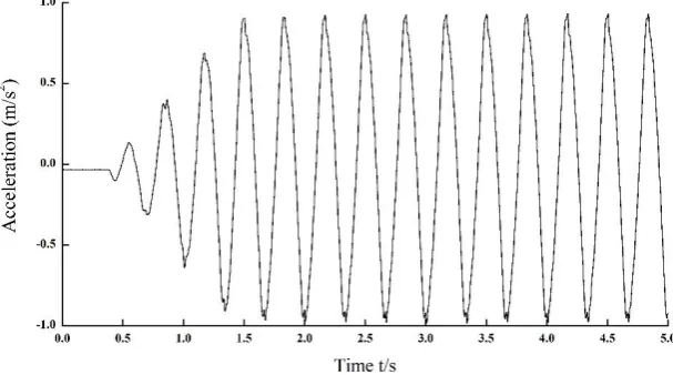
When the hydraulic servo shaking table without load is excited by a sinusoidal signal,
sin(2
3 )
t
m/s2, its corresponding sinusoidal acceleration response is shown in Figure 2. In time domain, it is clear that the acceleration response is not a standard sine wave but a distorted one. There are other seven harmonics (from the second to the eighth) except the fundamental frequency signal in the sinusoidal acceleration response shown in Figure 2 and Figure 3. Besides, in order to demonstrate the impact of the nonlinear hydraulic system, the total harmonic distortion (THD) is introduced. The value of THD can be calculated by using equation (1), and its analysis result is shown in Table 2. From Table 2, it can be seen that the amplitude of the fundamental response is less than the excitation signal. Besides, the third harmonic is the largest harmonic among other seven harmonics, i.e., it plays a most prominent part in THD. The amplitude of the sixth harmonic is the same as that of the Seventh, at 0.006, but both are less than the eighth harmonic. The fifth harmonic is in the least domination, at 0.016. The value of the THD is 7.06%.2 2 2
2 3
1
100% n
A A A
THD
A
+ + +
WhereA A1, 2, ,Anare the amplitude of each harmonic.
Figure 2. Acceleration response of sin(23t)m/s2 in time domain.
Figure 3. Acceleration response of sin(23t)m/s2 in frequency domain.
Table 2. THD analysis results.
THD Harmonic Amplitude (m/s2)
7.06% Fundamental Second Third Fourth Fifth Sixth Seventh eighth
0.859 0.005 0.057 0.004 0.016 0.006 0.006 0.008
3. Harmonic identification scheme based on Adaline-LMM algorithm
When the servo system is excited by a sinusoidal signal, the system response can be regarded as a composite signal which is composed of the fundamental response and high order harmonics. The general model of the composite signal can be defined as:
1
( ) isin( )
N
i i
a k A i k
=
=
+ (2)where, Ai,
i are the amplitude and phase of the ith harmonic, respectively.
is the fundamental frequency. N is the highest order of the acceleration harmonic. k represents iterations. For the purpose of obtaining the input vector of the network, equation (2) can be written as:1
( ) isin( ) cos( ) icos( ) sin( )
N
i i
i
a k A i k A i k
=
=
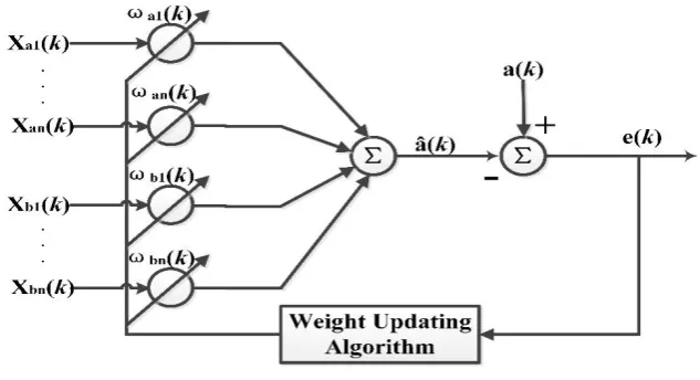
+ (3)(illustrated in Figure 4) is introduced. It is a single layer linear neural network which has n inputs but only a single output. The output of this neural network â(k) is the dot product between the input vector and weight vector. Certainly, the relationship between the output and the input of the neural network is linear at any time. The error signal e(k) will be acted as the input signal of the weight adjusting algorithm to adjust the weight of the Adaline. Apparently, with the output of the Adaline getting more and more close to the output of the servo system, this error signal is getting smaller too. That is, the process of training this neural network is actually the process that the output of the network converging to the expected signal.
Figure 4. Adaline neural network.
( )
ai
X k and Xbi( )k are input signal vectors of the network, and e(k) is the error signal which is used to adjust the weight of the network. Both
ai( )k and
bi( )k are the weight of the network. The above vectors are illustrated in equations. (4-6).X ( )ai k =sin(i k i
), =1, 2,3, ,n (4)X ( )bi k =cos(i k i
), =1, 2,3, ,n (5)e(k)=a(k)-â(k) (6)
The weight adjusting is accomplished by using the LMM algorithm, which is a nolinear algorithm using the error signal’s M-estimator so as to minimize the instantaneous criterion function JM( )k and then get the optimized weight vector. The criterion function JM( )k is
expressed as:
( ) { ( ( ))}
M
J k =E M e k (7)
where M(.) is a robust M-estimate function that can be obtained by using Hampel’s three parts re-descending function which is expressed as:
2
1
2 1
1 1 2
2 2
3
1 1 1
2 3
2 3
2 3
3
( )
0 ( )
2 ( ) ( ) 2 ( ( )) ( ( ) ) ( ) ( )
2 2 2
0 ( )
e k
e k t
h
t e k t e k t
M e k
e k h
h h h
h h t e k t
h h
t e k
− = − + − + − (8) ( ( ( ))) ( ( )) ( ( ))
M e k S e k
e k
=
(9)
1
1 1 2
1
3 2 3
2 3
3
( )
0
( )
sgn( ( ))
( )
( ( ))
[ ( )
]
sgn( ( ))
( )
0
( )
e k
e k
t
t
e k
t
e k
t
S e k
t
e k
t
e k
t
e k
t
t
t
t
e k
=
−
−
(10)where t1, t2 and t3 are thresholds used to control the impulse-suppressing degree and can be determined by estimating the variance of the impulse free signal. These threshold parameters can be estimated as[13]:
2 2 2 2 2
1 1 2
( )
k
C
(
k
1) (1
C C med e k
)
( ( ) , (
e k
1) ,... (
e k
L
w1) )
=
− + −
−
−
+
(11)1
2
3
1.96 ( ) 2.24 ( ) 2.57 ( )
t k t k t k
= = = (12)where ( )k is the estimated value of the variance of the impulse-free signal. C1 (C11) and C2
(2C23) are the active forgetting factor and the modifying factor, respectively. Lwrepresents the
length of the estimated window. Apparently, the stability and the tracing performance depend on these parameters.
When the criterion function JM( )k reaches the minimum value, the weight gets its optimized value. The first derivative of the criterion function is expressed as :
( ) ( ( )) ( ( )) ( )
( ) M ( ) ai
ai ai
J k M e k S e k X k
k k
= = −
(13)
( ) ( ( )) ( ( )) ( )
( ) M ( ) bi
bi bi
J k M e k S e k X k
k k
= = −
(14)
The update equation of the Adaline neural network’s weights are shown as:
( 1) ( ) ( )( ( ))
( )
ai ai ai M
ai
k k k J k
k
+ = + −
(15)
( 1) ( ) ( )( ( ))
( )
bi bi bi M
bi
k k k J k
k
+ = + −
(16)
Substituting equations (13-14) into equations (15-16), the weight update of the Adaline-LMM algorithm can be given as:
a
( 1) ( ) ( ( )) ( )
ai k ai k iS e k Xai k
+ =
+
(17)( 1) ( ) ( ( )) ( )
bi k bi k biS e k Xbi k
+ =
+
(18)where
ai,
bi represent variable weight updating steps which can be updated as:50
a 0.24
i
i bi
= = = (19)
where i is the number of iterations. If 0.0001, =0.0001.
When the LMM algorithm has been trained, the error signal will generally be very close to 0. At that time when the output of the network equals to the system’s output, the weight will not be adjusted. i.e., the ultimate weight vector is the Fourier coefficient vector of the signal. The ultimate weight vector can be given as:
1, 2, ,
[
]
a a a aN
=
(20)1, 2, ,
[
]
b b b bN
Due to equations (20-21), the ith harmonic’s amplitude and phase can be computed by:
2 2
( ( )) ( ( ))
i ai bi
A = k + k (22)
1
tan (
( ) /
( ))
iw k
biw k
ai
=
−(23)
4. Simulation results
The real-time and precision identification performance of the proposed Adaline-LMM algorithm is initially tested by simulation using MATLAB/SIMULINK. The simulation input is:
( )
(
)
(
)
(
)
(
)
(
)
(
)
a 3sin 1.2 0.6sin 2 0.9 0.5sin 3 0.7 0.4sin 4 0.5
0.3sin 5 0.4 0.2sin 6 0.3
k k k k k
k k
= + + + + + + +
+ + + + (24)
Apparently, there are 6 harmonics whose frequencies are the integral multiple of the fundamental frequency. Its sampling frequency is 1000Hz. The fundamental frequency is 3Hz. The optimum values of constant parameters such as C1, C2, Lw are 0.995, 2.157 and 12 respectively.
The initial values of both
ai( )k and
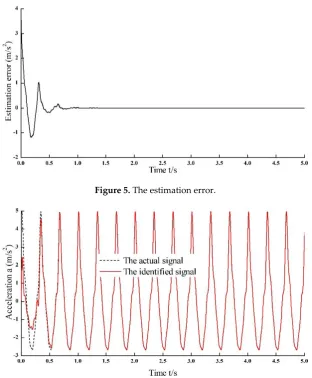
bi( )k are chosen as 0.018.From the error plot in Figure 5, it is noted that the estimation error is converging to nearly zero within 1s, in spite of much large fluctuation existing in the initial stage of harmonic identification. Figure 6 contains two different kinds of signals, both the actual signal denoted by dashed line and the identified signal denoted by red line. Although the estimation error is quite large originally, it is noted that the identified signal is well converged to the actual signal within 0.7s which means both the amplitude and the phase of each harmonic are precisely estimated.
Figure 5. The estimation error.
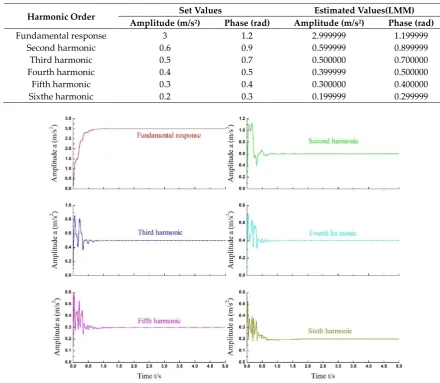
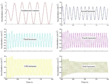
The estimation amplitude and phase of each identified harmonic are separately shown in Figure 7 and Figure 8, and the result of contrast between the estimated values and the set values is showed in Table 3. At the initial stage of the harmonic identification, there are relatively large fluctuation. But both amplitudes and phases of all the harmonics are converging to their specific values which are exactly the same as what the simulation input signal contains originally, i.e., the amplitude and phase of each harmonic are precisely estimated by using Adaline-LMM algorithm. Besides, harmonics can be directly identified and its results are shown in Figure 9.
Table 3. the result of contrast between the estimated values and the given values.
Harmonic Order Set Values Estimated Values(LMM)
Amplitude (m/s2) Phase (rad) Amplitude (m/s2) Phase (rad)
Fundamental response 3 1.2 2.999999 1.199999
Second harmonic 0.6 0.9 0.599999 0.899999
Third harmonic 0.5 0.7 0.500000 0.700000
Fourth harmonic 0.4 0.5 0.399999 0.500000
Fifth harmonic 0.3 0.4 0.300000 0.400000
Sixthe harmonic 0.2 0.3 0.199999 0.299999
Figure 8. Estimation phases of simulation results.
Figure 9. The identification harmonics.
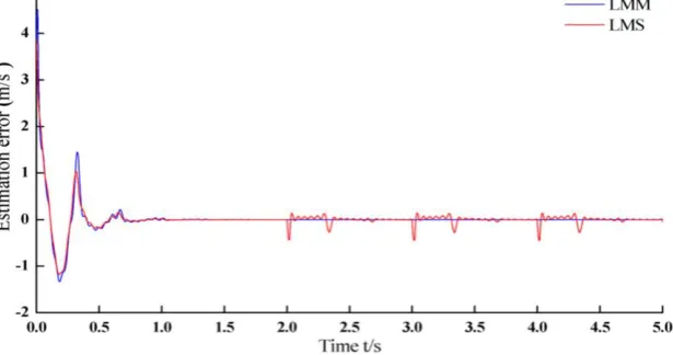
when impulse noise is acted in the input signal and there still has small oscillation after 2.5s, 3.5s and 4.5s(the action time of the impulse noise are 2s, 3s and 4s), but the estimation error is converged to zero and the error oscillation does emerge during the whole identification time.
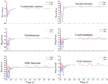
For simplicity in visualizing the merits of LMM, the identification results, both amplitude and phase of each harmonc, are separately shown in Figure 11 and Figure 12. It is noted that the identification amplitudes and phases are not steable and easy to be affected by the impulse noise which is not allowed in the acceleration harmonics identification for an electro-hydraulic servo shaking table. On the contrary, the amplitudes and phases estimated results by using LMM algorithm are more steable and not influenced by impulse noises. That is, unlike LMS algorithm, LMM can detect and ignore the impulse noise and provide a more steable and precise harmonic identification performance.
Figure 10. The estimation error when the input signal is contaminated by impulse noise.
Figure 12. Estimation phases of simulation result(contaminated by impulse noise).
5. Experiment results
For validating the effectiveness of the proposed algorithm for harmonic identification further, the real experiment is designed to test its identification precision. The initial values of
both
ai( )
k
and
bi( )
k
are chosen as 0.05. Its sampling frequency is also 1000Hz. During theexperiment, the Adaline-LMM parameters are kept as the same as the simulation except
L
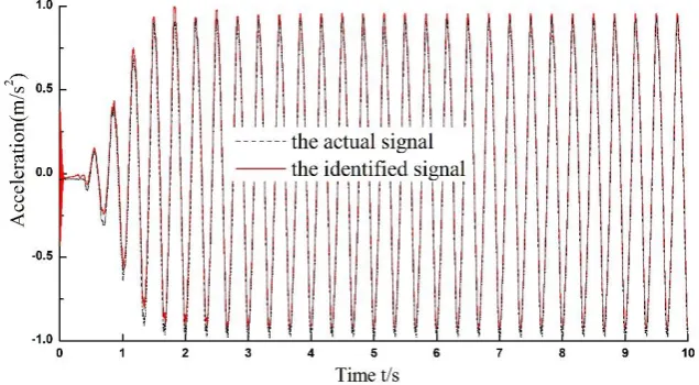
wwhich is set as 16. The estimation error is displayed in Figure 13 which is used to demonstrate the estimation accuracy. It is noted that the estimation error fluctuated largely at the beginning of the identification but rapidly converged to a relative small range(within 0.08) after 2s. There are two different lines, the dashed one is the system response signal and the red line presents the identification signal, contained in Figure 14. Originally, the red line has a wide fluctuation,
however, after the Adaline-LMM algorithm has been trained, ultimately, the identified signal is
well converged to the actual signal within 2s, i.e., the harmonic identification precision of the proposed algorithm is pretty great.
Figure 14. The process of harmonic identification in experiment.
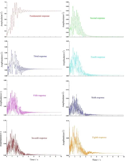
The estimation amplitude results are displayed in Figure 15. It is noted that the estimation amplitude values match well with the FFT-computed values which are shown in Table 2. As for the amplitude plots, all the amplitude values of harmonics are converged in the end. From the estimation phases shown in Figure 16, large fluctuations exist within initial 2 seconds, but, ultimately, they tend to be steady after around 4 seconds. However, there are still minor variations of the estimation phase existing in the second harmonic. Certainly, all of the harmonics can also be directed estimated online, and their waveforms are shown in Figure 17.
6. Conclusion
When the electro-hydraulic servo shaking table is excited by a sinusoidal signal, the system response contains high order harmonics due to many no-linear elements existing in this shaking table. For identifing each harmonic, both the amplitude and the phase, a no-linear adaptive algorithm based on a single layer ADALINE and LMM which is used to adjust the weights of the Adaline was proposed. Both the simulation and experimental results show that the proposed algorithm is able to identify the amplitude and phase of each harmonic online, and its real-time performance and precision have been proved to be satisfied.
Besides, the proposed ADALINE-LMM algorithm exhibits other characteristics like great tracing precision, fast convergence and simple algorithm construction. The most obvious advantage of this algorithm is that it can effectively dectect and ignore the impulse noises during the identification process. The simulation result shows that Compared with LMS algorithm, LMM algorithm is able to provide a more steable harmonic identification performance when the signal response is contaminated by impulse noise. Furthermore,the results from the proposed algorithm deserve to be studied further because they are not only useful for harmonic identification, but also for harmonic cancellation.
Author Contributions: Jianjun Yao proposed this acceleration harmonic identification scheme and directed other 4 co-authors to perform the experiment to validate its accuracy. Chenugang Xiao performed this harmonic identification experiment and wrote this paper. Zhenshuai Wan, Shiqi Zhang and Xiaodong Zhang did the data collection and processing works, and furthermore, revised the submitted paper.
Funding: This project is supported by National Natural Science Foundation of China (Grant No.51375102), and the Fundamental Research Funds for the Central Universities (Grant No. HEUCFP201733).
Figure 17. The identification harmonics of the experiment result.
References
1. H. R. Li, Hydraulic Control System, National Defense Industry Press, Beijing, (1990).
2. J. J. Yao, D. T. Di, G. L. Jiang, S. Gao and H. Yan, “Real-Time Acceleration Harmonics Estimation for an Electro-Hydraulic Servo Shaking Table Using Kalman Filter With a Linear Model”, IEEE Transactions ON Control Systems Technology, 22(2), 794-800, (2014).
3. J. J. Yao, G. L. Jiang, D. T. Di and S. Liu, “Acceleration harmonic identification for an electro-hydraulic servo shaking table based on the normalized least-mean-square adaptive algorithm”, Journal of Vibration and Control, 19(1), 47-55, (2013).
4. C.X. Cao, J.Y. Qian and L. X. He, “RBF Neural Network Application in harmonic detection”, Foreign Electronic Measurement Technology, 1, 46-47, (2007).
5. A. Ketabi, I. Sadeghkhani and R. Feuillet, “Using artificial neural network to analyze harmonic overvoltages during power system restoration”, European Transactions on Electrical Power, 21(7), 1941– 1953, (2011).
International Conference on Innovative Computing, Information and Control, 2, 379-382, (2006).
7. Y. X. Zou, S. C. Chan, and T. S. Ng. "A robust M-estimate adaptive filter for impulse noise suppression."
Acoustics, Speech, and Signal Processing, 1999. on 1999 IEEE International Conference IEEE Computer Society, 1999:1765-1768.
8. Wu, L. and Qiu, X., “An m-estimator based algorithm for active impulse-like noise control”, Applied Acoustics, 74(3), 407-412, (2011).
9. Zou, Y., Chan, S. C. and Ng, T. S., “Least mean m-estimate algorithms for robust adaptive filtering in impulse noise”, Circuits & Systems II Analog & Digital Signal Processing IEEE Transactions on, 47(12), 1564-1569, (2000).
10. G. Sun, M. Li and T. C. Lim, “Enhanced filtered-x least mean m -estimate algorithm for active impulsive noise control”, Applied Acoustics, 90, 31-41, (2015).
11. J. J. Yao, FU Wei, Sheng-Hai Hu and J. W. Han, “Amplitude phase control for electro-hydraulic servo system based on normalized least-mean-square adaptive filtering algorithm”, Journal of Central South University, 18(3), 755-759, (2011).
12. Yao, J., Dietz, M., Xiao, R., Yu, H., Wang, T. and Yue, D., “An overview of control schemes for hydraulic shaking tables”, Journal of Vibration & Control, 22(12), (2014).
13. Zou, Y. (2000). Robust statistics based adaptive filtering algorithms for impulsive noise suppression. HKU Theses Online (HKUTO).
14. Zheng, Z. and Zhao, H., “Affine projection m-estimate subband adaptive filters for robust adaptive filtering in impulsive noise ☆. Signal Processing”, 120(C), 64-70, (2016).
15. Chan, S. C. and Zou, Y. X., “Convergence analysis of the recursive least M-estimate adaptive filtering algorithm for impulse noise suppression”, International Conference on Digital Signal Processing, 2, 663-666, (2002).
16. Chan, S. C., Zou, Y. X. and Zhou, Y., “Comments on a recursive least m-estimate algorithm for robust adaptive filtering in impulsive noise: fast algorithm and convergence performance analysis”, IEEE Transactions on Signal Processing, 57(1), 388-389, (2009).
17. Yao, J., Wang, X., Hu, S. and Fu, W, “Adaline neural network-based adaptive inverse control for an electro-hydraulic servo system”, Journal of Vibration & Control,17(13), 2007-2014, (2011).
18. Chan, S. C. and Zhou, Y., “On the Convergence Analysis of the Normalized LMS and the Normalized Least Mean M-Estimate Algorithms”, IEEE International Symposium on Signal Processing and Information Technology, 1048-1053, 2007.
19. Ray, P. K. and Subudhi, B., “Bfo optimized rls algorithm for power system harmonics estimation”, Applied Soft Computing, 12(8), 1965-1977, (2012).
20. Yao, J. J., Hu, S. H., Fu, W. and Han, J. W., “Impact of excitation signal upon the acceleration harmonic distortion of an electro-hydraulic shaking table”, Journal of Vibration & Control, 17(7), 1106-1111, (2011). 21. Belega, D., Petri, D. and Dallet, D., “An effective procedure for the estimation of harmonic parameters of
distorted sine-waves”, Instrumentation and Measurement Technology Conference , 8443, 1429-1434, (2012).