ISSN: 2251-8436 print/2322-1666 online
BAYES AND EMPIRICAL BAYES ESTIMATION OF
PARAMETER k IN NEGATIVE BINOMIAL
DISTRIBUTION
MASOUD GANJI∗, NASRIN EGHBALI AND MASOUD AZIMIAN
Abstract. In this paper, the problem of estimating the number
of successes,k, in a negative binomial distribution for both known and unknown probabilitypof success are examined by a Bayesian point of view. Also, we introduce two estimations for the parameter of negative bionomial distribution.
Key Words: Bayes estimation, negative binomial distribution, Empirical Bayes estimation, hyper parameter.
2010 Mathematics Subject Classification:Primary: 13A15; Secondary: 13F30, 13G05.
1. Introduction
Let X1, X2, ..., Xn be a random Variables of size n from a negative binomial distributionN B(K, P), whereK and P are independent. The probability density function (briefly, pdf) of Xi is
(1.1) f(xi|k, p) =
(
xi+k−1 xi
)
pk(1−p)xi,
xi = 0,1,2, ... , k∈ {1,2,3, ...}, p∈(0,1).
The negative binomial distribution is an univariate discrete proba-bility model with one variable, that has many applications in different fields such as ecology, biology and genetics. Also for modeling count data with over dispersion (that is sample variance exceeds the mean
Received: 7 April 2013, Accepted: 11 October 2013. Communicated by H. R. Nilisani ∗Address correspondence to Masoud Ganji; E-mail:[email protected]
c
⃝2013 University of Mohaghegh Ardabili.
sample), a popular and convenient model is the negative binomial dis-tribution (see [1], [2], [3]). The usual problem in the negative binomial situation is to estimate the probability of successp. However, in other instances, the number of success k may be the unknown parameter. There are different ways to estimate this parameter, for example the method of moments estimation (MME), maximum likelihood estima-tion (MLE) and the Bayes method. Many researchers in each turn, have obtained estimations for parameters of negative binomial distribution. For example, Piegorsch [9] used the maximum likelihood estimation for parameterk in this distribution; Clark and Perry [3] used the moment and maximum extended quasi-likelihood estimators for estimationkand Adamids [1], used the EM algorithm for the parameters of the negative binomial distribution. These methods are classical methods. Ganji [6], in a more general case, investigated Bayes estimation of parameters of generalized negative binomial distribution and it’s applications; he has fixed the parameterk and then estimated the parameterp (probability of success). In this research, we are going to estimate the parameterk. We are interested in Bayes and Empirical Bayes estimations of param-eterk in two cases of known and unknown parameterp. We consider a left-truncated prior distribution forkand a beta prior distribution forp
and suggest choosing values for the hyper parameters of the prior distri-bution. In Section 2, we describe the probability models that are needed in this work. Bayes estimations forkare proposed in section 3. Empiri-cal Bayes estimations fork are investigeted in section 4. We provide an example in section 5. In section 6 simulation study are presented.
2. The Models
LetX1, X2, ..., Xn∼N B(k, p) and the pdf ofXi is given in (1.1). The likelihood function of{x1, x2, ..., xn} given k≥1 and p, is given by:
(2.1) L(x1, x2, ..., xn|k, p) = n ∏ i=1
(
xi+k−1 xi
)
pnk(1−p) n ∑ i=1
xi
.
SinceKis the number of success in the negative binomial experiment, sok≥1. We consider a left-truncated distribution forK for which the probability density function, is given by:
(2.2) g(k) = e
−λλk
where the hyper parameterλis a preselected integer that is chosen to re-flect our beliefs about the expected value ofk, because the expected value ofkequals approximatelyλ. In order to construct the Bayes estimation for k, the posterior pdf of K given the observations{x1, x2, . . . , xn} is derived in this section under the assumption of known and unknown p, separately.
2.1. Case1: p is unknown. Assume thatpis an unknown parameter. A suitable prior distribution for p is the beta distribution with hyper parameters alpha and beta, that is P ∼beta(α, β). The prior pdf of P
is given by:
(2.3) w(p) = Γ(α+β) Γ(α)Γ(β)p
α−1(1−p)β−1; p∈(0,1)
where the hyper parameters α and β are preselected positive numbers that should be chosen according to our beliefs about the expected value of the truep, because the expected value ofp equals α+αβ. If we believe that the actual value of thepis small, less than 0.5 then, let αα+β <1/2 , therefore, it is recommended to setβ > α. If the actual value of thep
is moderate, around 0.5, then α+αβ = 1/2, therefore, it is recommended to set β =α, and if the the actual value of the p is large, greater than 0.5, then α+αβ >1/2, therefore it is recommended to set β < α.
It is mentioned that in Bayesian Statistics we use the Bayes rule to obtain posterior distribution. Here we introduce this rule in the following theorem.
Theorem 2.1. (Bayes rule) Let A1, A2, ... be a partition of the sample
space, and let B be any set. Then for each i= 1,2, ..., p(Ai|B) =
p(B|Ai)p(Ai)
∞
∑ j=1
p(B|Aj)p(Aj)
.
Now for a parameter θ, if we denote the prior distribution by π(θ) and the sampling distribution byf(x|θ), then the posterior distribution of θfor the given sample x is:
π(θ|x) = f(x|θ)π(θ)
m(x) , wherem(x) is the marginal distribution ofX, that is
m(x) = ∫
In this case, the parameterp is unknown, so we have two parameters
k and p in the probability density function of Xi. Now to obtain the Bayes point estimation for this parameters, we have to first find the joint posterior pdf ofK andP:
Lemma 2.2. The joint posterior pdf of K and P given observations {x1, x2,· · · , xn}, is given by:
(2.4)
h(k, p|x1, ..., xn) = C11pnk+α−1(1−p)Tn+β−1λ k
k!
n ∏ i=1
(
xi+k−1
xi )
.
where Tn= n ∑ i=1
xi and C1 is normalizing constant:
(2.5) C1=
∞ ∑ k=1
λk k!
Γ(Tn+β)Γ(nk+α)
Γ(Tn+β+α+nk) n ∏ i=1
(
xi+k−1 xi
) ,
Proof. Using theorem 2.1 we have:
h(k, p|x1, x2, ..., xn) =
L(x1, x2, ..., xn|k, p)g(k)w(p) ∫1
0 ∞
∑ k=1
L(x1, x2, ..., xn|k, p)g(k)w(p)dp = 1
C1
pα+kn−1(1−p)Tk+β−1λ
k
k! n ∏ i=1
(
k+xi−1
xi )
.
□
Lemma 2.3. The marginal posterior pdf of K given observations {x1, x2,· · · , xn},
is given by:
(2.6) hK(k|x1, ..., xn) = C11λ k
k!
Γ(nk+α)Γ(Tn+β) Γ(nk+α+Tn+β)
n ∏ i=1
(
xi+k−1 xi
)
,
Proof. By taking the integral ofh(k, p|x1, x2, ..., xn) overp, the marginal
density function ofK is obtained:
hK(k|x1, x2, ..., xn) = ∫ 1
0
h(k, p|x1, x2, ..., xn)dp = 1
C1 λk k!
n ∏ i=1
(
k+xi−1
xi )
Γ(kn+α)Γ(Tn+β) Γ(α+β+Tn+kn)
.
□
Lemma 2.4. The marginal posterior pdf of P given observations {x1, x2,· · ·, xn},
is given by:
(2.7) hP(p|x1, ..., xn) = CC2(1p)pα−1(1−p)Tn+β−1, where k≥1, p∈(0,1) andC2(p) =
∞
∑ k=1
(pnλ)k
k!
n ∏ i=1
(
xi+k−1 xi
)
. Proof. The proof is similar to the proof of the Lemma 2.3, but here we
have to replace the integral by sum. □
Since the likelihood function L(x1, x2,· · ·, xn|k, p) is less than one and, also the prior g(k) and w(p) are proper, so the denominator of
h(k, p|x1, x2, . . . , xn) which equalsC1, is less than 1. So the normalizing
constant C1 is convergent. Similarly, the convergence of C2(p) can be
obtained. As a result C1 and C2(p) can be approximated by the finite
sums:
(2.8) C1=
z ∑ k=1
S(k),
and
(2.9) C2(p) =
q ∑ k=1
Y(k),
whereS(k) = λkk!Γ(nk+α)Γ(Tn+β) Γ(nk+α+Tn+β)
n ∏ i=1
(xi+k−1 xi
)
, Y(k) = (pnkλ!)k n ∏ i=1
(xi+k−1 xi
) ,
zis the first integer that satisfies the inequality|S(z+ 1)−S(z)|⩽ϵand
q is the first integer that satisfies in the inequality|Y(q+ 1)−Y(q)|⩽ϵ; whereϵ is a very small positive number, for instance 10−6.
2.2. Case 2: p is known: Suppose that p is known. In this case the posterior pdf ofK is given in the following Lemma:
Lemma 2.5. The posterior pdf ofK given observations{x1, x2,· · · , xn} andp, is given by:
(2.10) hK(k|x1, ..., xn, p) = C21(p)(p
nλ)k
k!
n ∏ i=1
(
xi+k−1 xi
)
, where k ≥ 1 and C2(p) is the normalizing constant defined in Lemma
2.4.
Proof. Using Theorem 2.1, the posterior density function of K is ob-tained:
hK(k|x1, ..., xn, p) =
L(x1, ..., xn|k, p)g(k)
∞
∑ k=1
L(x1, ..., xn|k, p)g(k)
= 1
C2(p)
(pnλ)k
k! n ∏ i=1
(
xi+k−1 xi
)
.
□
2.3. Case 2: p is known: Suppose that p is known. In this case the posterior pdf ofK is given in the following Lemma:
Lemma 2.6. The posterior pdf ofK given observations{x1, x2,· · · , xn} andp, is given by:
(2.11) hK(k|x1, ..., xn, p) = C21(p)(p
nλ)k
k!
n ∏ i=1
(
xi+k−1 xi
)
, where k ≥ 1 and C2(p) is the normalizing constant defined in Lemma
2.4.
Proof. Using Theorem 2.1, the posterior density function of K is ob-tained:
hK(k|x1, ..., xn, p) =
L(x1, ..., xn|k, p)g(k)
∞
∑ k=1
L(x1, ..., xn|k, p)g(k)
= 1
C2(p)
(pnλ)k
k! n ∏ i=1
(
xi+k−1 xi
)
□
3. Bayes Point Estimation of k
In this section, Bayes estimation forkare proposed under the squared error loss function, that is the mean of the posterior density function. Both cases, known and unknownp are considered, separately.
3.1. Case1: pis Unknown. Assume thatpis an unknown parameter. Lemma 3.1. The Bayes point estimation (kˆ1) of k is:
(3.1) kˆ1= Γ(TCn1+β) ∞
∑ k=1
kλkk!Γ(TΓ(nk+α) n+β+α+nk)
n ∏ i=1
( xi+k−1
xi
)
.
Proof. As it is mentioned, the Bayes point estimation of k under the squared error loss function is the the mean of the marginal posterior pdf of kin (2.6). So we have:
ˆ
k1 =EhK(K)
=
∞
∑ k=1
khK(k|x1, ..., xn) = Γ(Tn+β)
C1 ∞ ∑ k=1 kλ k k!
Γ(nk+α) Γ(Tn+β+α+nk)
n ∏ i=1
(
xi+k−1
xi )
.
□
Bayes point estimation ofp is given in the following results: Lemma 3.2. The Bayes point estimation (pˆ1) ofp is:
(3.2) pˆ1 = Γ(TCn1+β) ∞
∑ k=1
λk
k!
Γ(nk+α+1) Γ(Tn+β+α+nk+1)
n ∏ i=1
(xi+k−1 xi
)
.
Proof. Bayes point estimation ofpunder the squared error loss function is the mean of the marginal posterior pdf of p in (2.7). So we have:
ˆ
p1=EhP(P)
= ∫ 1
0
php(p|x1, ..., xn)dp = Γ(Tn+β)
C1 ∞ ∑ k=1 λk k!
Γ(nk+α+ 1) Γ(Tn+β+α+nk+ 1)
n ∏ i=1
(
xi+k−1
xi )
.
3.2. Case 2: p is known: Assume thatp is a known parameter. Lemma 3.3. The Bayes point estimation (ˆk2) of k is:
(3.3) ˆk2= C21(p) ∞
∑ k=1
k(pnkλ!)k
n ∏ i=1
(xi+k−1 xi
)
.
Proof. Bayes point estimation ofkunder the squared error loss function is the mean of the marginal posterior pdf ofk in (2.10). So we have:
ˆ
k2 =EK(k)
=
∞
∑ k=1
kK(k|x1, ..., xn, p)
= 1
C2(p) ∞
∑ k=1
k(p
nλ)k
k! n ∏ i=1
(
xi+k−1
xi )
.
□
It should be mentioned that the proposed Bayes estimations ˆk1, ˆk2
and ˆp1 are finite because the priors ofk andpare proper with the finite
mean, and the likelihood is bounded by one. Wald [7] showed that, Bayesian posterior mean estimations that arise from proper priors, are always admissible. So ˆk1, ˆk2 and ˆp1 are admissible estimators.
4. Empirical Bayes Estimation of k
In this section, a procedure for constructing empirical Bayes estima-tions forkis provided in both cases: known and unknownp, separately.
M M E technique is used to estimate the hyper parameters λ,α and β. 4.1. Case 1: p is unknown. By evaluating
∫1 0
∑∞
k=1f(x|k, p)g(k)w(p)dp,
where f(x|k, p), g(k) and w(p) are defined in (1.1), (2.2) and (2.3) re-spectively, the marginal pdf of X, is:
fX(x) = ∫ 1
0 ∞
∑ k=1
f(x|k, p)w(p)g(k)dp
= Γ(α+β) Γ(α)Γ(β)
∞
∑ k=1
(
x+k−1
x
)
× e−λλk k!(1−e−λ)
Γ(α+k)Γ(β+x) Γ(x+β+α+k).
It is difficult to calculate the moments by using the pdf ofX, so in the following Lemma we obtain it:
Lemma 4.1. First, second and third moment ofX are:
(4.1)
E(X) = λ (1−e−λ)
β
(α−1),
E(X2) = λ (1−e−λ)
β
(α−1)[1 + (2 +λ)
(β+ 1) (α−2)],
E(X3) = λ (1−e−λ)
β
(α−1)[1 + (6 + 3λ)
(β+ 1) (α−2) +(λ2+ 6λ+ 6)(β+ 2)(β+ 1)
(α−3)(α−2)].
Proof. Using the well-known identity EX(X) = EK,P[E(X|k, p)], first,
second, and third moment of X are obtained. □
In order to construct the empirical Bayes estimation fork, it is neces-sary to estimate the hyper parametersλ,αandβ. TheM M Evalues for
λ,α andβ can be obtained by solving the following system of nonlinear equations:
(4.2)
E(X) =
n ∑ i=1
Xi
n ,
E(X2) =
n ∑ i=1
X2 i
n ,
E(X3) =
n ∑ i=1
X3 i
n .
The empirical Bayes estimation ˆk1(emp) is same as Bayes estimation ˆk1
in (3.1), but here, hyper parameters λ,α and β are replaced by M M E
values.
4.2. Case 2: p is known: By evaluating ∑∞k=1f(x|k, p)g(k), where
f(x|k, p) and g(k) are defined in (1.1) and (2.2) respectively, the mar-ginal pdf of X is:
(4.3) fX(x) =
∞ ∑ k=1
(
x+k−1
x )
pk(1−p)x e
−λλk k!(1−e−λ).
In this case in order to obtain the empirical bayes estimation of k, we have to estimate the hyper parameterλ, so the M M E ofλis obtained in the following lemma.
Lemma 4.2. TheM M E of λis:
(4.4) λˆ =
pTn+ (1−p)nΩ(−pTne
− pTn (1−p)n (1−p)n )
(1−p)n ,
where Tn = n ∑ i=1
Xi and Ω(A) is the product log function A, which is defined as the value of x that satisfies the equationxex=A.
Proof. Using the well-known identity EX(X) = EK,P[E(X|k, p)], first moment ofX is obtained and theM M E ofλis obtained by solving the following equation:
(1−p)
p
λ
1−e−λ = n ∑ i=1
Xi
n .
□
The empirical Bayes point estimation ˆk2(emp) is ˆk2, defined in (3.3)
with ˆλinstead ofλ.
It should be mentioned that, since k is an integer, the nearest integer for the proposed estimations ˆk1, ˆk1(emp), ˆk2, and ˆk2(emp) is taken as
the estimator ofk.
5. Illustrative Example
Example 5.1. Let {23,29,47,25,54} be a random sample of sizen= 5 that was generated using Mathematica7 fromN B(20,0.4). Suppose that
α=β = 1 and λis assumed to be 23. The marginal posterior pdf of k given the sample{23,29,47,25,54}, is given by:
hK(k|23,29,47,25,54) = C1
1 λk
k!
Γ(5k+1)Γ(179) Γ(5k+180)
(k+22
23
)(k+28
29
)(k+46
47
)(k+24
25
)(k+53
54
)
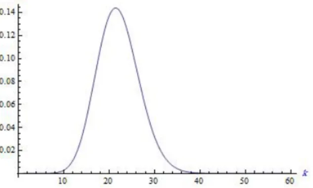
Figure 1. Plot of S(k) in 2.8 for the Example 5.1 where
C1 = ∞
∑ k=1
S(k)⋍ z ∑ k=1
S(k) = z ∑ k=1
23k
k!
Γ(5k+1)Γ(179) Γ(5k+180)
(k+22
23
)(k+28
29
)(k+46
47
) (k+24
25
)(k+53
54 ) = 40 ∑ k=1 λk k!
Γ(5k+1)Γ(179) Γ(5k+180)
(k+22
23
)(k+28
29
)(k+46
47
)(k+24
25
)(k+53
54
) = 1.66.
Hence, the marginal posterior pdf ofK is:
hK(k|23,29,47,25,54) = 1.16623
k
n!
Γ(5k+1)Γ(179) Γ(5k+180) ×
(k+22
23
)(k+28
29
)(k+46
47
) (k+24
25
)(k+53
54
)
,
so whenpis unknown, the Bayes estimation ofkis given by the following sum:
ˆ
k1 ⋍ 1.166 40
∑ k=1
k23k!kΓ(5Γ(5k+1)Γ(179)k+180) ×(k+2223 )(k+2829 )(k+4647 )
(k+24
25
)(k+53
54
)
= 22.0264.
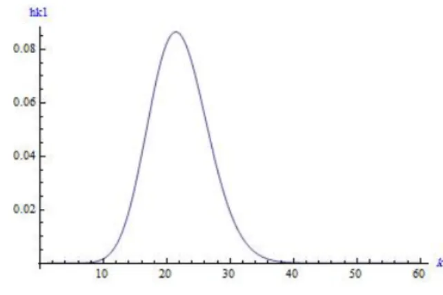
In order to choose z for notice after equation 2.8 and 2.9 had expressed, we design the plot of S(k) in figure 1 and we see after point 40 plot is flat, so we choose 40 that satisfy |S(41)−S(40)| ⩽ 10−6. Also for calculating ˆk1 for notice Figure 2 that shows the values ofhK(k) when
p is unknown we see that after point 40 this values are almost 0 so in calculating ˆk1 we choose the point 40. The posterior distribution fork
Figure 2. plot of posterior pdf hK(k) when p is un-known for Example 5.1
k 1 · · · 6 · · · 10 11 12 13
hK(k) 7.72e−11 · · · 0.000021 · · · 0.0017 0.0035 0.0068 0.012
k 14 15 16 17 18 19 20 21
hK(k) 0.02 0.03 0.04 0.053 0.065 0.075 0.082 0.086
k 22 23 24 25 26 27 28 29
hK(k) 0.0859 0.082 0.075 0.065 0.053 0.04 0.03 0.02
k 30 · · · 35 40 45 50 60 >60
hK(k) 0.0068 · · · 0.0035 0.0017 0.000021 7.72e−11 7.02e−11 0.0000
Table 1. Values of marginal posterior of example 1 when p is unknown
When p is known, the marginal posterior pdf of K given sample
{23,29,47,25,54}, is given by:
hK(k|23,29,47,25,54) = C21(p)(p 5λ)k
k!
(k+22
23
)(k+28
29
)(k+46
47
)(k+24
25
)(k+53
54
)
,
where
C2(p) = ∞
∑ k=1
Y(k)⋍ q ∑ k=1
Y(k) = q ∑ k=1
(23×0.45)k
k!
(k+22
23
)(k+28
29
) (k+46
47
)(k+24
25
)(k+53
54
) =
40
∑ k=1
(23×0.45)k
k!
(k+22
23
)(k+28
29
)(k+46
47
)(k+24
25
)(k+53
54
) = 3.4292×1040.
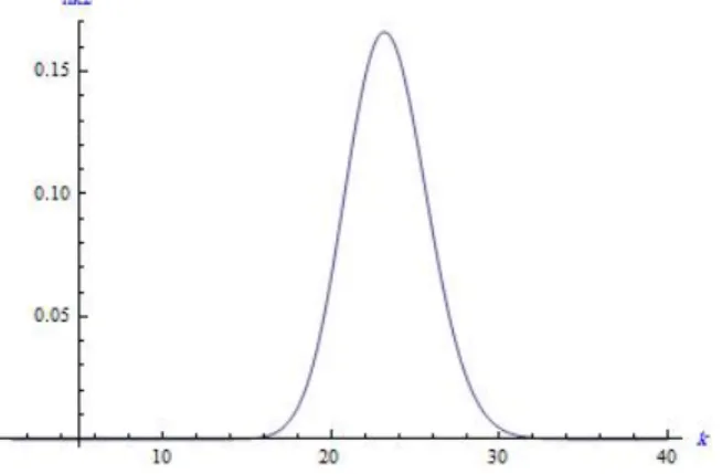
Figure 3. Plot of Y(k) in 2.9 for the Example 5.1
Figure 4. plot of posterior pdfhK(k) whenp is known for Example 5.1
So when p is known, the Bayes estimator of k (ˆk2) is given by the
following sum: ˆ
k2= 3.4292×101 40
40
∑ k=1
k(23×k0!.45)k(k+2223 )(k+2829 )(k+4647 )(k+2425 )(k+5354 )
= 23.32.
Note that choosingq is similar to choosingz in case of unknownp. The values of posterior distribution for k, when p is known are given in the table 2.
k 1 · · · 6 · · · 10 11 12
hK(k) 6.86e−42 · · · 3.5e−19 · · · 1.18e−10 6.38e−9 1.43e−7
k 13 14 15 16 17 18 19
hK(k) 2.16e−6 0.000023 0.00017 0.00094 0.0039 0.01279 0.03254
k 20 21 22 23 24 25 26
hK(k) 0.06614 0.1089 0.1474 0.1656 0.1563 0.1250 0.08549
k 27 28 29 30 31 32 33
hK(k) 0.05038 0.02577 0.01152 0.0045 0.00157 0.00048 0.000135
k 34 35 · · · 40 50 60 >60
hK(k) 0.000033 7.47e−6 1.0092e−9 · · · 4.89e−20 5.058e−33 0.0000
Table 2. Values of marginal posterior of example 1 when p is known
When p is unknown, the empirical Bayes estimation ˆk1(emp) can’t
be calculated, because solving the system of nonlinear equation in (4.3) gives bad estimation for the hyperparametersα,β andλ, so we omitted this estimator.
When p is known, as we said, the empirical Bayes estimation ˆk2(emp)
is obtained by replacing ˆλin (4.5) withλin ˆk2; that is, ˆλ= 23.73. So:
ˆ
k2(emp) = 7.12718×101 40
40
∑ k=1
k(23.73k×!0.45)k(k+2223 )(k+2829 )(k+4647 )(k+2425 )(k+5354 )
= 23.505.
6. Simulation Study
In this section, the performance of the proposed estimators of k is investigated through a simulation study. The simulation study is carried out for different values of the combinations (n, k, p). In this study, in the case of knownp, we suggested the ˆλ= 1Xp¯−p to calculating the estimator ˆ
k2, that we choose this value for hyperparameter λ, since if 100(1− p) percent of the number of trials is failure, so 100p leaving of trials are the number of success(k). Hence by a simple proportion we have ˆ
λ = 1Xp¯−p and by using this value for λ we obtained good estimator similar of that in empirical estimator. It has to mentioned that, in this proportion we replace thekbyλ, because in prior distribution its mean is equal toλapproximately. In these cases we have generated 500 random
k n θ
0.2 0.5 0.8
10 5(0.6) 5(1.01) 5(2.62) 5 20 5(0.32) 5(.43) 5(1.37) 30 5(.197) 5(0.33) 5(0.85) 10 20(2.32) 20(3.97) 20(10.013) 20 20 20(1.34) 20(1.8) 20(4.92)
30 20(0.75) 20(1.25) 20(3.28) 10 48(4.61) 46(18.43) 47(16.32) 50 20 49(2.30) 48(8.8) 47(9.8)
30 49(1.56) 48(6.67) 48(5.73)
Table 3. expected and MSE valuses of the stimator ˆ
k2(emp) for k whenp is known
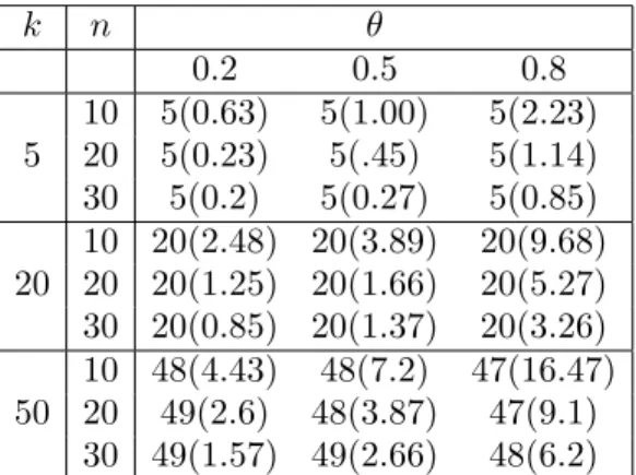
k n θ
0.2 0.5 0.8 10 5(0.63) 5(1.00) 5(2.23) 5 20 5(0.23) 5(.45) 5(1.14) 30 5(0.2) 5(0.27) 5(0.85) 10 20(2.48) 20(3.89) 20(9.68) 20 20 20(1.25) 20(1.66) 20(5.27) 30 20(0.85) 20(1.37) 20(3.26) 10 48(4.43) 48(7.2) 47(16.47) 50 20 49(2.6) 48(3.87) 47(9.1)
30 49(1.57) 49(2.66) 48(6.2)
Table 4. expected and MSE valuses of the estimator ˆk2
forkwhen p is known
sample of size n(= 10,20and30) from a negative binomial distribution with parametersp(= 0.2,0.5and0.8) andk(= 5,20and50) by using the mathematica 7. In order to see how the estimators of k perform with respect to sample size, the average value of estimators ˆk2(emp) and ˆk2
along with MSE in parentheses are reported in Table 3 and Table 4, respectively. From tables 3 and 4, we see that when θ increases, the MSE also increases. For each k, when the size of sample is increased, then the MSE decreases.
Acknowledgments
The authors thank the referee for his (her) helpful comments.
References
[1] K. Adamids,An EM Algoritm for estimation negative binomial parameters, Aus-tralian New zealand Journal of Statistics,41(2) (1999), 213–221.
[2] N. Breslow,Extra-Poisson variation in log-linear models, Applied Statistics,33 (1984), 38–44.
[3] S. J. Clark and J. N. Perry,Estimation of the negative binomialparameter k by maximum quasi-likelihood, Biometrics,45(1989), 309–316.
[4] G. Casella and R. L. Berger, Statistical Inference, Duxbury Thomson Learning Publishing, (2001).
[5] J. Engel, Models for respons data showing extra-poisson variation, Statistical Neerlandica,38(1984), 159–167.
[6] M. Ganji,Bayes estimation of parameters of generalized negative binomial dis-tribution and it’s applications, Iranian Journal of Science and Technology (in persion),3,4(2005), 47–53.
[7] J. F. Lawless,Negative Binomial and mixed poisson regression, Canadian Jornal of Statistics,15(1987), 209–225.
[8] K. G. Manton, M. A. Woodbury, and E. Stallard,A variance components approch to categorical data models with heterogeneos cell populations: Analysis of spatial gradiants in lung canser mortality rates in North Carolina counties., Biometrics, 37(1981), 259–269.
[9] W. W. Piegorsch, Maximum likelihood estimation for the negative binomial dis-persion parameterk, Biometrics,46(1990), 863–867.
[10] A. Wald,Statistical Decision Functions. Wiley , New York, (1950).
Masoud Ganji
Department of Statistics, Facualty of Mathematical Sciences, University of Mohaghegh Ardabili, 56199-11367, Ardabil, Iran.
Email: [email protected]
Nasrin Eghbali
Department of Mathematics and Applications, Facualty of Mathematical Sciences, University of Mohaghegh Ardabili, 56199-11367, Ardabil, Iran.
Email: [email protected];[email protected]
Masoud Azimian
Department of Statistics, Facualty of Mathematical Sciences, University of Mohaghegh Ardabili, 56199-11367, Ardabil, Iran.