TREASURY WORKING PAPER
01/32
Saving and growth in an open economy
Iris Claus, David Haugh, Grant Scobie
and Jonas Törnquist
Abstract
Concern has been raised by an apparent lack of saving in New Zealand. It is often argued that policies which foster savings are important, as higher savings will contribute to higher economic growth. This paper investigates the link between saving, investment and growth. In particular, it focuses on issues potentially important in an open economy such as New Zealand. Theory predicts that increased total saving will lead to higher investment and output. In an open economy, total saving comprises saving by domestic agents (government, firms and households) plus foreign saving. Diversified portfolios, large inflows of foreign investment into New Zealand and investment rates comparable to those in other OECD countries suggest that New Zealand, so far, has been able to access foreign saving to meet investment demands. Domestic saving does not appear to have constrained investment and hence growth.
JEL classification: E21, E22, O16
Keywords: Economic growth, saving, capital flows
Corresponding author: Iris Claus, The Treasury, P.O. Box 3724, Wellington, New Zealand, email: [email protected], telephone: 64 4 471 5221. David Haugh, The Treasury, P.O. Box 3724, Wellington, New Zealand, email: [email protected], telephone: 64 4 471 5233. Grant Scobie, The Treasury, P.O. Box 3724, Wellington, New Zealand, email: [email protected], telephone: 64 4 471 5005. Jonas Törnquist, The Treasury, P.O. Box 3724, Wellington, New Zealand, email: [email protected], telephone: 64 4 471 5265.
CONTENTS
1 Introduction ...2
2 The link between saving, investment and growth ...2
3 Access to foreign capital ...9
4 How does New Zealand compare to other OECD countries? ...15
5 The New Zealand experience...18
6 Concluding remarks ...31
References...32
Appendix: Definition of ratings...35
List of figures Figure 1: The Solow-Swan model...5
Figure 2: Growth rate of income per efficiency worker ...5
Figure 3: Supply and demand of loanable funds...13
Figure 4: Net national saving, investment and the current account (all as a percentage of GDP) and real GDP growth...17
Figure 5: Saving, investment and real GDP growth in New Zealand ...18
Figure 6: Impulse responses (in percent)...22
Figure 7: Proportion of New Zealand government bonds held for non-residents....23
Figure 8: New Zealand household holdings of domestic and foreign equity...24
Figure 9: New Zealand’s current account and Standard and Poor’s Ratings Group foreign currency credit rating ...26
Figure 10: New Zealand’s current account and Moody’s Investors Service foreign currency credit rating ...26
Figure 11 : Total foreign investment (as a percentage of GDP, three-year moving average) ...28
Figure 12: Equity liabilities versus borrowing ...30
Figure 13: General government versus corporate borrowing (dollar millions)...30
List of tables Table 1: Share of foreign equities in total equity portfolios (end of 1996)...11
Table 2: Feldstein-Horioka equation for New Zealand ...19
Table 3: Granger causality tests ...20
SAVING AND GROWTH IN AN OPEN ECONOMY *
1 INTRODUCTION
It is often argued that policies which foster saving are important as higher saving will contribute to higher economic growth. The purpose of this paper is to investigate the link between saving, investment and growth, with particular focus on issues potentially important in a small open economy such as New Zealand. The main conclusion of the paper is that domestic saving does not appear to have constrained investment and hence growth in New Zealand. The corollary is that it is unlikely that higher levels of domestic saving would lead to higher investment and improved growth. Promoting growth would not alone provide justification for interventions to raise domestic saving. The remainder of the paper is organised as follows. Part 2 establishes the theoretical link between saving, investment and growth. Part 3 discusses issues potentially relevant in open economies: access to world financial markets, the home bias in equity holdings (or, more generally, in overall asset positions), the saving-investment puzzle of Feldstein and Horioka (1980) and the sustainability of current account deficits. Part 4 compares saving and investment rates, the current account and real output growth across selected OECD countries and Part 5 considers the New Zealand experience in more detail, with particular focus on the points discussed in Part 3. Concluding remarks are contained in Part 6.
2 THE LINK BETWEEN SAVING, INVESTMENT AND GROWTH Some accounting identities1
In a closed economy, ex post, the value of a country’s gross domestic product equals gross national expenditure, i.e. all goods and services are absorbed domestically. Total absorption consists of government consumption (G), household consumption (C), and firms’ investment (I). In an open economy, total spending by residents comprises the absorption of domestically produced goods and services and goods and services produced abroad. The difference between residents’ spending on domestically produced goods and services and total absorption is imports (M). Exports (X) are foreign spending on domestically produced goods and services. If the trade balance is in deficit, i.e. imports exceed exports, absorption (A) exceeds output (Y), i.e.
M X A
Y− = − (2.1)
where A = G + C + I. The current account balance (CAB) is defined as the sum of the trade balance (X – M), net income paid abroad (ya) and net transfers paid abroad (t)
* The authors would like to thank Maryanne Aynsley, Bob Buckle, David Galt, Lesley Haines, Viv Hall, Gary Hawke, Leslie Hull, Geoff Lewis, Struan Little, Nathan McLellan, Dorian Owen and Les Oxley for valuable comments. The paper has also benefited of comments from participants at the Victoria University of Wellington symposium “Sustainable and excessive current account deficits” (November 2001). Special thanks are due to Claire Gardiner and Graham Howard for their assistance in obtaining data.
t y M X
CAB= − + a + (2.2)
where net income paid abroad (ya) plus consumption of fixed capital (or depreciation) is
the difference between the gross domestic product (Y) and national income (Yn).
The link to saving and investment is as follows. Gross saving (S) is the difference between GDP and consumption by households and the government (C + G). Gross domestic investment is the difference between total absorption and consumption, i.e.
M X I S ) G C A ( ) G C Y
( − − − − − = − = − (2.3)
Equation (2.3) hence implies that when the trade balance is in deficit, imports exceed exports and gross domestic investment exceeds gross saving. Moreover, it can be shown that the difference between domestic saving (Sd) and net domestic investment
(Inet) is equal to the current account balance CAB
I
Sd − net = (2.4)
where domestic saving (Sd) is the difference between national disposable income (Y d)
and government and household consumption, and net investment (Inet) is gross
domestic investment net of depreciation. Disposable income (Yd) is the difference
between national income (Yn) less net transfers paid abroad (t).2
In a closed economy, domestic saving must equal investment ex post. In an open economy, the difference between domestic saving and net domestic investment is the current account balance. When the current account balance is in deficit, the excess of net domestic investment over saving is financed by foreign funds or net capital inflows as measured by net foreign investment or the capital account surplus. In other words, an economy with access to foreign capital can augment its capital stock through foreign investment. An increase in the stock of capital, in turn, will increase output as discussed in the next section.
The theoretical link
The (closed-economy) neoclassical growth model of Solow (1956) and Swan (1956) is a useful starting point for establishing the theoretical link between saving, investment and growth. Despite its rudimentary demand structure and neglect of international borrowing and lending, it yields useful insights into the effects of saving, technological advance and population growth. In particular, the Solow-Swan model shows that an increase in the stock of capital leads to a higher level of output and faster growth at least in the short to medium term. Once the new level of output is reached, growth returns to its initial level. This result carries over to more complicated models.
The Solow-Swan model of long-run economic growth consists of a production function, which relates the inputs in the economy to the outputs produced, and a capital accumulation equation, which describes how capital accumulates in the economy. The production function is assumed Cobb-Douglas with constant returns to scale in capital
2 This follows from S – I – ya – t = Y – C – G – ya – t – I = Yn + ya + d – C – G – ya – t – I = Yd + t + d – C – G – t – I = (Yd – C – G) – (I – d) = X – M – ya – t = CAB for CAB < 0, where d denotes consumption of fixed capital.
(K ) and labour (t L ); that is doubling the inputs, t K and t L , leads to double the output, t
t
Y , i.e. α − α = 1 t t t
t A K L
Y (2.5)
where A is an exogenous productivity parameter and t 0<α<1 is the income share of capital. Note that the production function has diminishing returns in capital (labour); that is doubling capital (or labour) alone increases output by less than double.
Because domestic saving must equal domestic investment in a closed economy, capital accumulation is given by
t t t 1
t K sY dK
K + − = − (2.6)
where sY denotes private saving (i.e. saving is a fixed fraction s of current income t
t
Y ) and d is the rate of depreciation.
The two key engines of growth in this model are exogenous technological change and labour force expansion. Productivity is assumed to grow at a constant rate g
t 1
t (1 g)A
A+ = + (2.7)
and the labour force, which equals population, grows at rate n
t 1
t (1 n)L
L + = + (2.8)
Because productivity and the labour force are growing, the steady states will not be stationary and output, for example, will grow. To express the system in terms of stationary steady states, the capital accumulation equation (2.6) is normalised by dividing by AtLt, the two exogenous variables in the system that are trending
t t t t t t t t t t t 1 t L A dK L A sY L A K L A K − = −
+ (2.9)
or ) k ) d ) g 1 )( n 1 (( sy ( ) g 1 )( n 1 ( 1 1 k
kt 1 t t − + + + t
+ + + = −
+ (2.10)
where k and t y are capital and output per “efficiency worker” (t AtLt).3
The link between saving, capital and output can be illustrated with the Solow diagram. Figure 1 plots the production function, y , the saving function, sy , and savings needed to maintain any given level of capital, ((1+n)(1+g)+d)k, all as a function of capital per
3 This follows from k (1 g)(1 n) L A L A L A K L A K 1 t t t 1 t 1 t 1 t 1 t 1 t t t 1
t = = + +
+ + + + + + + .
efficiency worker, k . Time subscripts are dropped as the diagram describes the long run. The savings function and savings needed to maintain a given level of capital intersect at the long-run equilibrium, steady state, where capital accumulation is zero, point (k*, y*).
Figure 1: The Solow-Swan model
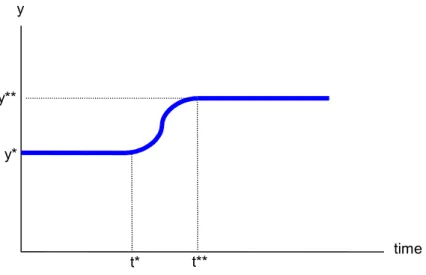
The Solow diagram can be used to investigate how changing the saving rate affects the economy. For example, consider the effect of an increase in the saving rate from s to 's . The steady state capital per efficiency worker increases from k* to k** and income per efficiency labour rises from y* to y**. However, once the economy adjusts to its new level of capital, it resumes its former growth rate. This can be seen in Figure 2, which plots income per efficiency worker over time.
Figure 2: Growth rate of income per efficiency worker k y
y
sy ((1+g)(1+n)+d)k
s'y
k* k** y*
y**
time y
y* y**
Prior to the increase in the saving rate, the ratio of income to efficiency labour (y*) is constant (∆y* = 0); that is income grows at the same rate as efficiency labour. The increase in the saving rate leads to an increase in the efficiency labour capital stock from k* to k** and income from y* to y** (Figure 1). To move to the higher equilibrium stock of capital k**, capital must grow faster for some time than efficiency labour, i.e. the ratio of capital to efficiency labour is increasing. Because of faster capital stock accumulation, income will also temporarily grow faster than efficiency labour. However, once the new steady state (k**, y**) is reached, capital and income will grow again at the same rate as efficiency labour, i.e. y** is constant. This implies that a country willing to invest more of its output (and consume less) can enjoy a temporary growth spurt; however, increased savings will not raise growth indefinitely.
One unrealistic simplification in the Solow-Swan model is that the saving rate is determined exogenously. Saving decisions are determined by agents’ rate of time preference and reflect intertemporal trade-offs. Although higher savings lead to higher per capita income and a higher growth rate in the short and medium term, welfare is not necessarily enhanced. This is because the gain occurs at the expense of current consumption.
In the Ramsey model as constructed by Ramsey (1928), Cass (1965) and Koopmans (1965), the path of consumption and hence the saving rate are determined endogenously, by optimising households and firms who interact on competitive markets subject to intertemporal budget constraints. In the Ramsey and other optimising models, there is also a positive link between saving and output, i.e. increased savings lead to increased output through capital accumulation. However in these models, the saving rate, in general, is not constant like in the neoclassical Solow-Swan growth model, but is instead a function of the per efficiency labour capital stock. These optimising models (both representative agent and overlapping generations models) are thus consistent with the empirical evidence that suggests that saving rates typically rise with per capita income (discussed further in Part 4) and are probably a more accurate description of the real world.4
The models discussed so far generally take technological change as exogenous and simply assume technological progress grows along a constant path. In contrast, “endogenous growth models” focus on understanding the economic forces underlying technological progress. Leading this research was P. Romer (see Romer 1986 and 1990). The 1986 Romer model endogenises technological progress by allowing for externalities (or positive spillover effects), while the 1990 model explicitly takes into account research and development.
The result that changes in the investment rate (or saving rate) have no long-run effect on economic growth also holds for the Romer model. Changes in the rate of saving or investment affect the growth rate along a transition path to the new steady state altering the level of income. But again, once that level is reached, the growth rate resumes its initial rate.
In contrast to the neoclassical and Romer models, where increased saving does not have a long-run impact on economic growth, the AK model predicts that there will be a
4 For more details on the Ramsey and other optimising agents models see Barro and Sala-i-Martin (1995).
permanent change through capital deepening (see Jones 1998).5 The reason the AK model has this characteristic is because the production function has constant returns to scale in capital. The production function in the AK model sets α in equation (2.5) equal to 1 and is given by
t
t AK
Y = (2.11)
where the level of technology, A, is assumed to be some positive constant (rather than time dependent).
In the AK model, an increase in the saving rate will have a permanent effect on the rate of growth of the economy. Higher saving increases capital and a larger capital stock leads to higher growth. This is because the marginal rate of return to capital is positive even as the capital stock grows infinitely large6
0 A K Y lim
K = >
∂ ∂ ∞
→ (2.12)
However, the empirical evidence does not support the AK model and it is unlikely that a country can sustain indefinite growth in per capita income through capital deepening. Constant returns to scale would imply that the exponent on capital was 1. Conventional estimates of the capital share using growth accounting suggest that the capital share is about 1/3. If one broadens the concept of capital to include human capital and externalities like “learning by doing” or other positive externalities due to the presence of ideas and technology, the exponent becomes 2/3 or maybe 4/5, but there is little evidence to suggest that the coefficient is 1.
Foreign saving7
In a small open economy, where capital is mobile, investment is not constrained by domestic saving as firms have access to foreign saving. With an infinitely elastic supply of foreign funds does it matter for growth whether capital is accumulated from domestic or foreign saving?
In an open economy, the production function is given by ) L , K , K , A ( f
Yt = t d,t f,t t (2.13)
where, as before, A is a productivity parameter. Two sources of capital are t distinguished: K denotes domestically sourced capital and d,t K is foreign sourced f,t capital. L denotes labour. t
The sources of output or gross domestic product growth can be identified by the total differential of equation (2.13), i.e.
5 The AK model takes its name after its production function, see equation (2.11). 6 In the case of the Cobb-Douglas production function, 0
K Y lim K Y lim K
K =
α = ∂ ∂ ∞ → ∞ → .
dL ) L , K , K , A ( f dK ) L , K , K , A ( f dK ) L , K , K , A ( f dA ) L , K , K , A ( f dY f d L f f d K d f d K f d A f d + + + = (2.14)
where dAfA(.) , fKd(.)dKd, fKf(.)dKf and fL(.)dL denote the partial derivatives with respect to A , K , d K and L respectively. Time subscripts are dropped for simplicity. f However, because some of the output must be paid to foreigners for the use of their capital, national income (Yn) is less than output (Y) by the interest cost paid for the use
of foreign capital. National income is thus given by
f w
n Y r K
Y = − (2.15)
Equation (2.15) assumes that the economy is small and faces an infinitely elastic supply of capital on the international market at the world interest rate (r ). For w simplicity, we also abstract from a country risk premium.
Growth of national income (after allowing for payments to foreigners) can be written as
f w
n dY r dK
dY = − (2.16)
or 4 4 3 4 4 2 1 4 4 4 4 4 3 4 4 4 4 4 2
1A K d L K w f
n f (.)dA f (.)dK f (.)dL (f (.) r )dK
dY
f
d + + −
+
= (2.17)
domestic sources foreign sources
Equation (2.17) shows that an increase in foreign investment will enhance national income if the term (fK (.) rw)dKf
f − is positive. In other words, provided the return on
foreign capital (adjusted for depreciation) exceeds the rate of interest paid on foreign borrowing, foreign investment will raise the level of the domestic country’s national income. Both national income and output growth in the borrowing country will be higher than it would have been in the absence of the foreign capital flow.8
Does an inflow of foreign capital decrease domestic saving? In the absence of open capital markets, the domestic interest rate will exceed the world rate. Thus, opening the economy to international capital movements will result in a lower rate of interest domestically. The domestic interest rate will be equal to the world rate plus an adjustment for a country risk premium.
The effect of access to foreign capital and lower domestic interest rates on saving is theoretically ambiguous. This is because lower interest rates make current consumption less expensive in relation to future consumption, and hence consumption would be expected to rise and domestic saving to fall (the substitution effect). However, at the same time, lower interest rates reduce household income from interest
payments and will encourage greater saving (the income effect).9 Which of these two effects dominates can only be determined empirically. Much of the evidence is uncertain. Generally, the interest rate sensitivity of domestic saving is found to be small. This suggests that domestic saving may be little affected by the presence of foreign saving.
Access to foreign capital makes the borrowing country unambiguously better off. Savings decisions are determined by agents’ rate of time preference and intertemporal trade-offs. International capital movements allow a country to consume more in future while maintaining current consumption. Increasing domestic saving would lower interest paid to foreigners for the use of their capital, but not necessarily increase welfare. This is because higher savings imply lower consumption. However, it is clear that the reduced interest payments to foreigners would increase national income in future.
Theoretical models of growth predict that higher saving and investment will result in a higher level of per capita income and temporarily faster growth. But once the new level of income is reached, the growth rate will resume its initial rate. There is little empirical evidence for models that predict that increased saving has a long-run effect on economic growth.
In a closed economy, investment is constrained by domestic saving. In an open economy, where capital is mobile, domestic saving and investment can diverge without necessarily impeding growth. When a country’s trade balance is in deficit, imports exceed exports and gross domestic investment exceeds gross domestic saving. The question then becomes “Is capital sufficiently mobile?”.
3 ACCESS TO FOREIGN CAPITAL
A necessary condition for access to foreign capital is the existence of integrated financial markets. Substantial theoretical and empirical work has investigated the role of financial markets in economic growth and development.10 Using different measures of financial depth indicators covering the banking sector, and the stock and bond markets, various empirical studies have found a significant relationship between financial development and growth across countries. That is, more developed countries have more developed financial markets.11
Feldstein and Horioka (1980)
In a well-known paper, Feldstein and Horioka (1980) claim that even among industrial countries, capital mobility is sufficiently limited so that investment rates ultimately depend on domestic saving rates. As evidence, they report cross-section regressions of average gross domestic investment rates on gross national saving rates for a sample of 16 OECD countries over the period 1960-74. The results show a slope coefficient of close to 1 (0.887). Feldstein and Horioka argue that a coefficient of close
9 For borrowers, lower interest rates that reduce interest payments encourage greater current consumption and less saving, i.e. the income and substitution effect operate in the same direction.
10 For a recent review of the literature see Khan and Senhadji (2000). 11 See, for example, King and Levine (1993) and Khan and Senhadji (2000).
to 1 indicates that “most of the incremental saving in each country has remained there”. If capital markets were indeed highly mobile, the slope coefficient would be much smaller than 1, as a country’s saving would tend to seek out the most productive investment opportunities worldwide. As a consequence, risk adjusted interest rates would tend to equalise.
The empirical results produced by Feldstein and Horioka are in contrast to other evidence that capital is quite mobile and the similar rates of interest on comparable assets that are observed across a range of industrial countries. This casts doubt on the robustness of these results. Over the period 1960-74, capital was not as mobile internationally as today, and Obstfeld and Rogoff (1996) show that the Feldstein-Horioka results are much weaker (0.62) for a sample of 22 OECD countries over the period 1982-91.
Taylor (1994) finds that the Feldstein-Horioka results might be the result of omitted variable bias. Controlling for (i) relative price effects, (ii) the age structure of population, and (iii) the interaction of the age structure with the growth rate of domestic output, the cross-sectional saving-investment relationship disappears.12
Another interpretation of the Feldstein-Horioka results is that the high coefficient on saving is due to specific individual country effects rather than low mobility. Using three different panel data estimation procedures and data for a group of ten OECD countries for the period 1885-1992, Corbin (2001) provides evidence of this hypothesis.
Home bias in equity portfolios
While the Feldstein-Horioka claim that domestic investment is ultimately determined by domestic saving is probably an over-simplification, “home bias” in equity portfolios does suggest that there may be some barriers to capital mobility. Research on international portfolio choice consistently predicts that investors should put much more of their wealth into foreign assets than they actually do; i.e. investors appear to engage in a sub-optimal degree of international diversification (see Glassman and Riddick 2001). This “home bias” in investors’ equity portfolios occurs despite rapid growth of international capital and equities markets and may be evidence that capital, at least in the form of equity, is not very mobile internationally.13
When French and Poterba (1991) first reported on the home bias portfolio puzzle, they found that at the end of the 1980s, Americans held about 94 percent of their equity wealth in the U.S. stock market. The proportion of domestic equity in Japanese and British investors’ portfolios was about 98 and 82 percent respectively.
The home equity bias may be somewhat less important for some smaller countries and has shown some tendency to decline over time (Tesar and Werner 1998). By the end of 1996, about 10 percent of U.S. equity wealth was invested abroad, while the proportion of foreign equity in Japan and the United Kingdom rose to 5.3 and 22.5 percent (Table 1). The share of foreign equity in Canada and Germany was about 11.2 and 18.2 percent respectively.
12 Feldstein and Horioka (1980) used saving and investment as shares of output at domestic prices. This ignores that it is changes in relative prices that affect decisions about real quantities of consumption and investment.
Table 1: Share of foreign equities in total equity portfolios (end of 1996)
Canada 11.2 Japan 5.3 Germany 18.2 United Kingdom 22.5
United States 10.0
Source: Rowland and Tesar (2000)
The reasons for home bias in equity portfolios are not well understood. Trading costs are unlikely to be the reason as the turnover rate on non-resident holdings of equity appears to be greater than the turnover rate for resident owners (see Tesar and Werner 1995). Other potential explanations range from information asymmetries, differential tax treatment of domestic and foreign equities and the significant share of nontradeables in most countries’ output.14
The nontradeables explanation is as follows. Suppose people can trade shares of future national outputs. They can also trade claims on other countries’ output of nontradeables. But because nontradeables cannot cross national borders, a foreign owner of such a claim must be paid in tradeables.
The optimal share of a country’s nontraded goods industries held domestically depends on the utility function. If, as is commonly assumed, the utility function is additively separable in the consumption of tradeable and nontradeable goods, then, in equilibrium, all claims to a country’s nontraded output will be held domestically.15 In other words, once people have fully diversified their portfolios of claims to tradeables, they cannot gain further by diversifying their holdings of nontradeables (Obstfeld and Rogoff 2000). This implies that if, say, 50 percent of total output consists of tradeables, then about half of investors’ portfolios should be held abroad.16
Sustainability of the current account
The discussion in Part 2 showed that the difference between domestic saving (Sd) and
net domestic investment (Inet) is equal to the current account balance. Those countries
who are “net savers” will lend to those who are “net borrowers”. This intertemporal borrowing and lending achieves faster accumulation of investment and a more efficient allocation of global capital. Both lending and borrowing countries stand to gain from these capital flows and the associated foreign investment. The availability of foreign funds depends, in part, on the sustainability of the current account. Sustainability of the current account, in turn, depends on the ability to generate sufficient trade surpluses in future to repay existing debt and the willingness of foreign investors to continue lending (Milesi-Ferretti and Razin 1996).
14 Informational asymmetries and the “lemons problem” are discussed further below.
15 An additively, separable utility function implies that the marginal utility of consumption of the tradeable good does not depend on consumption decisions about the nontradeable good and vice versa.
16 Determining the optimal share of nontraded goods industries held domestically becomes more complicated for the case of non-separable preferences (see, for example, Baxter, Jermann and King 1998).
! Intertemporal solvency
A country is solvent if the present discounted value of its future trade surpluses equals its current account indebtedness or net external debt. A country’s current account deficit is sustainable if the solvency condition holds (assuming everything else constant). In other words, sustainability implies that the external debt does not increase without limits.
In the presence of economic growth, persistent current account deficits can be consistent with solvency, provided that future trade surpluses are sufficiently large. This result is derived as follows. As noted in Part 2, the current account balance (CAB) is the sum of the trade balance (X – M), net income paid abroad (ya) and net transfers
paid abroad (t). For simplicity, we assume that net transfers paid abroad equal zero. Alternatively, the current account balance can be written in terms of stocks, as the change in net foreign assets (NFA)
t t t a t t t 1
t NFA X M y X M rNFA
NFA + − = − + = − + (3.1)
where r denotes the rate of interest paid on foreign debt (assumed constant over time); and hence rNFA equals net income paid abroad. t
Equation (3.1) can be written as17
(
s s)
ts
t s
t X M
r 1 1 NFA ) r 1 ( − + = + − − ∞ =
∑
(3.2)It states that the present value of an economy’s net resource transfer to foreigners, i.e. future trade balances (X – M), must be equal to the value of the economy’s initial debt to foreigners. Thus, a country’s intertemporal budget constraint holds if, and only if, the country pays off any initial foreign debt through sufficiently large future surpluses in its balance of trade.
However, it can be shown that an economy with growing output can have persistent current account deficits that are sustainable. A country’s current account will be sustainable in the long run if the foreign debt to output ratio is constant. Suppose that long-run, steady state output (Y ) grows at rate g, i.e. s
s 1
s (1 g)Y
Y+ = + (3.3)
If the country’s current account is sustainable, i.e. the debt to output ratio is stable, then external debt will also grow at g
s 1
s (1 g)NFA
NFA + = + (3.4)
17 This follows from
NFA t = (1 + r)(– (X t – M t) + NFA t+1) = – (1 + r)(X t – M t) + (1 + r)(1 + r)(– (X t+1 –
M t+1) + NFA t+2 ) =
(
s s)
1 t s t s M X r 1 1 − + − + − ∞ =∑
.This implies that for a current account deficit to be an equilibrium, the country only needs to pay the difference between the interest rate and its growth rate18
s s s
s s
Y NFA ) g r ( Y
) M X
( − = − − (3.5)
! Willingness of foreign investors to lend
The availability of foreign funds is also determined by the willingness of international investors to lend to a net debtor country. One important factor determining a country’s supply of external finance is the (mean) rate of return on domestic assets, which is likely to be influenced by the expected growth performance of the borrowing country. The supply of foreign funds, in turn, determines the cost of foreign borrowing to the domestic country.
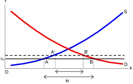
In a small open economy the supply of foreign funds is infinitely elastic and the cost of borrowing is determined by the world interest rate (plus some country risk premium). Figure 3 plots the supply and demand of loanable funds as a function of the interest rate in a small open economy. For simplicity, we assume that the country risk premium is zero.
Figure 3: Supply and demand of loanable funds
The demand curve for capital is downward sloping and given by D. The “domestic” supply curve of loanable funds is determined by domestic saving and given by S. The world interest rate is denoted by rw and, because the risk premium is assumed to be
zero, determines the cost of borrowing of firms. At rate rw, domestic lenders will supply
OA of capital and foreign lenders will provide AB.
Domestic firms’ cost of borrowing will increase or decrease with changes in the world interest rate or changes in the country’s risk premium. If the world interest rate rises because of a decline in world saving and/or the country’s credit (or exchange rate) risk
18 This follows from NFAs+1−NFAs =g⋅NFAs =(Xs −Ms)+r⋅NFAs.
r
k S
D rw
kf
A
A' B'
B O
increases, the cost of borrowing increases. Conversely, the cost of borrowing will fall if the size of the world portfolio increases or the country’s risk premium declines.19
With no distortions, markets will always clear. However, in a world with imperfect information, lenders may not always be willing to lend. Capital markets may not always clear and credit rationing can occur. Credit rationing means that some borrowing countries may not be able to borrow even if they offered to pay a premium above world rates (see Stiglitz and Weiss 1981). International investors may be unwilling to lend at higher interest rates because higher interest rates increase the average riskiness of investment projects. Higher interest rates increase the probability of making a “bad loan”. This is because those, who are willing to pay high interest rates, may, on average, be worse risks. They are willing to borrow at high interest rates because they perceive their probability of repaying the loan to be low.20
A decline in the supply of foreign capital and increase in the cost of borrowing is unlikely to be fully offset by higher domestic saving. To offset a shortfall in foreign saving the domestic supply of loanable funds curve would need to shift downward. This would only occur if domestic savers were prepared to supply the same amount of saving at a lower rate of interest, at the same time when the world interest had risen. This seems improbable, and hence it is unlikely that domestic saving will increase enough to make up for the decline in foreign saving. If domestic saving does not increase, then domestic investment and output will fall following a decline in the supply of foreign capital.
Foreign debt versus foreign equity
There are two broad categories of foreign investment: debt and equity. The corporate finance literature on the optimal capital structure of firms provides a useful starting point for discussion. Under the assumption that (i) financial markets are complete and (ii) information and transaction costs are non-existent, the Modigliani and Miller (1958) theorem states that the mix of debt and equity used to finance firms’ expenditures is irrelevant to the choice of investment project. In other words, whether a firm finances its investments with debt or equity does not affect the expected profitability of an investment project – the same investment decisions would be made, irrespective of the mix of debt and equity finance.
However, information and transactions costs do exist because of an information asymmetry between borrowers and lenders. Borrowers generally know more about their investment projects than lenders. The most famous illustration of the problems caused by asymmetric information is Akerlof’s (1970) “lemons” problem. Equity will be under-priced since investors will be suspicious of the fundamentals of any firm that is willing to sell an equity share. Because of the lemons problem, a “good” firm would prefer to issue debt rather than equity. Thus, firms with the highest credit rating will
19 Figure 3 also shows how the opening of capital market increases the supply of funds available to domestic firms and hence output. The “autarky” stock of capital is determined where the demand and domestic supply curves intersect. Access to world capital markets lowers the cost of borrowing and increases firms’ capital stock.
20 Higher interest rates may also induce firms to undertake projects with lower probabilities of success but higher payoffs when successful. Increasing the rate of interest increases the relative attractiveness of riskier projects, for which the return to the lender may be lower.
issue bonds first and then equity if external finance is required.21 Some firms with a high credit rating will also choose to issue equity to avoid unnecessary bankruptcy in a world of uncertainty where firms are subject to unforeseen shocks.
The information asymmetry is likely to be augmented in the presence of open capital markets because of additional informational asymmetries between foreign and domestic investors. One way to reduce or overcome the informational asymmetries between foreign investors and domestic firms is foreign direct investment (FDI). This is because purchasing a controlling interest in a firm allows the foreign investor to gain full insight into the firm’s business. One would thus expect FDI to dominate other forms of global finance in countries where information asymmetries between foreign and domestic investors are particularly important.
Because of the “lemons” premium, raising capital through equity financing or foreign direct investment is more costly than issuing bonds. However, as noted before there may be other motivations for equity financing. For example, equity allows for greater risk sharing. In the case of foreign direct investment foreign investors will bear part of the country’s risk in the event of a negative shock. Foreign direct investment may also improve productive efficiencies by allowing countries to better exploit sectoral comparative advantages (Hull and Tesar 2000b). In addition, it can involve technological spillover or transfer of technology and entrepreneurial skills. Bosworth and Collins (1999) examine 58 developing countries from 1978-95 and find that one dollar of foreign direct investment is associated with an additional 50 cents of domestic investment.
4 HOW DOES NEW ZEALAND COMPARE TO OTHER OECD COUNTRIES? The remainder of the paper considers the empirical link between saving, investment and growth in New Zealand. We start by briefly comparing the New Zealand experience to that in other selected OECD countries.
Figure 4 plots net national saving, total gross fixed capital formation (investment), the current account, all as a percentage of GDP, and real GDP growth for 12 selected OECD countries: Australia, Canada, Finland, Germany, Ireland, Japan, Korea, New Zealand, Norway, Sweden, the United Kingdom and the United States. The series were obtained from the OECD national accounts database, except for New Zealand. Data for New Zealand were constructed from Statistics New Zealand official data.22 Data are plotted from 1972 to 2001.
21 If firms can also borrow from banks, they will prefer issuing debt to equity to borrowing from banks. This is because bank borrowing incurs intermediation costs (see Hull and Tesar 2000a).
22 SNA93 data for New Zealand are only available from 1987 onwards. Prior to 1987 data were constructed by splicing on the growth rates of the SNA68 series to the levels of the SNA93 series, apart for real GDP. The GDP measure prior to 1987 is a “calibrated” chain data series. Quarterly SNA93 chain-linked data were regressed on the fixed weight SNA68 data for the period for which both were available (June 1987 to June 2000). Parameter estimates from this regression were then used to derive an estimate of the chain series from the fixed series for the period from September 1977 to March 1987 for which the fixed series but not the chain series is available.
! Saving
Figure 4 shows that saving rates have varied substantially across OECD countries. Saving has been lowest in Finland, with an average rate of 1 percent of GDP, while Korea and Japan experienced the highest average rates, at around 21 and 18 percent respectively. Saving has also been relatively high in Norway, at around 12 percent of GDP. In the rest of the countries, saving rates have averaged between around 4 percent (New Zealand) and 9 percent (Germany). Moreover, net national saving was lower over the 1990s compared to the 1970s and 1980s in Australia, Canada, Germany and New Zealand.
! Investment
While New Zealand’s measured saving rate is lower than in other OECD countries, this does not appear to have affected investment. In fact, New Zealand’s average investment rate at around 22 percent ranks in the middle of OECD rates, which range from around 30 percent (Korea and Japan) to slightly less than 19 percent for the United Kingdom and the United States. Norway’s average investment rate is also high, with about 26 percent.
Overall, investment rates have been fairly stable in Australia, Canada, Germany, Japan, New Zealand, the United Kingdom and the United States. In contrast, in Finland and Sweden, they appear to have dropped to a lower level in 1993. Moreover, investment has been quite volatile in Ireland, Korea and Norway, steadily declining in Norway and trending upward in Korea. In Ireland, the investment rate fell over much of the 1980s, but rose over the 1990s.
! Current account
Although Korea has had high (and rising) investment rates, domestic saving has been sufficient to meet strong investment demand. As a result, its current account as a percentage of GDP, on average, has been zero. The current account also has fluctuated around zero in Germany, Finland and Sweden. In Finland and Sweden, the current account was in deficit until 1993; however, since then, current account surpluses have offset previous deficits. The relatively small current account deficit in Finland prior to 1993 and balanced current account over the period as a whole is somewhat surprising, given Finland’s high rates of investment and low saving rates. The current account in Australia, Canada, Ireland, New Zealand, the United Kingdom and the United States has been in deficit. Ireland’s current account reached a trough at –13 percent of GDP in 1981; however, since 1987 it has shown a small surplus. In Australia, Canada and New Zealand, the current account has been in deficit, associated with relatively low rates of net national saving. In the United Kingdom and the United States, both investment and saving rates have been low.
Japan and Norway, on average, have had current account surpluses. High rates of investment have been more than offset by high rates of net national saving.
Figure 4: Net national saving, investment and the current account (all as a percentage of GDP) and real GDP growth
Source: OECD, Statistics New Zealand and The Treasury.
Current account as a percent of GDP Net national saving as a percent of GDP Investment as a percent of GDP Real GDP growth
Australia -15 -10-5 0 5 10 15 20 25 30 35 40
1972 1979 1986 1993 2000
Canada -15 -10-5 0 5 10 15 20 25 30 35 40
1972 1979 1986 1993 2000
Finland -15 -10-5 0 5 10 15 20 25 30 35 40
1972 1979 1986 1993 2000
Germany -15 -10-5 0 5 10 15 20 25 30 35 40
1972 1979 1986 1993 2000
Ireland -15 -10-5 0 5 10 15 20 25 30 35 40
1972 1979 1986 1993 2000
Japan -15 -10-5 0 5 10 15 20 25 30 35 40
1972 1979 1986 1993 2000
Korea -15 -10-5 0 5 10 15 20 25 30 35 40
1972 1979 1986 1993 2000
New Zealand -15 -10-5 0 5 10 15 20 25 30 35 40
1972 1979 1986 1993 2000
Norway -15 -10-5 0 5 10 15 20 25 30 35 40
1972 1979 1986 1993 2000
Sweden -15 -10-5 0 5 10 15 20 25 30 35 40
1972 1979 1986 1993 2000
United Kingdom -15 -10-5 0 5 10 15 20 25 30 35 40
1972 1979 1986 1993 2000
United States -15 -10-5 0 5 10 15 20 25 30 35 40
! Real GDP growth
Average real GDP growth has varied across countries between 2-2.5 percent (Canada, Germany, Japan, Sweden, New Zealand and the United Kingdom) and around 7 percent (Korea). At 5.4 percent, average real output growth also has been high in Ireland. In Australia, Finland, Norway and the United States real output growth has fluctuated around 3 percent.
These numbers and Figure 4 show that there is no obvious empirical link between domestic saving, investment, the current account and real output growth. For example, Japan has experienced high rates of saving and investment (and a current account surplus), but its real output growth rates have been relatively low. Korea has also had high saving and investment rates, but its real output growth rates have been high (and the current account balanced). In contrast, Finland’s saving rate has been very low, but its average growth rate comparable to those in other OECD countries.
5 THE NEW ZEALAND EXPERIENCE The Feldstein and Horioka claim
To examine the empirical link between domestic saving, investment and real output growth in more detail for New Zealand, we first estimate the Feldstein-Horioka equation, discussed in Part 3.
Data used in the estimation are the same as in Part 4 except for investment. Investment is gross fixed capital formation in plant machinery and equipment plus residential and non-residential building. The measure of investment excludes other construction, transport equipment, intangible fixed assets and land improvements. This is because the null hypothesis of a unit root in the ratio of total gross fixed capital formation to (nominal) GDP could not be rejected at conventional levels of significance. The ratio of saving to output and real GDP growth are stationary at conventional levels of significance. Figure 5 plots the data. The estimation period is 1980 to 2000.
Regressing the ratio of investment to output against a constant and the ratio of saving to output using ordinary least squares (OLS) produces a slope coefficient on the saving rate of 0.564. However, the equation is mis-specified. The Durbin and Watson (1951) statistic, which tests for first-order serial correlation in the residuals, rejects the null hypothesis of no positive autocorrelation.
Figure 5: Saving, investment and real GDP growth in New Zealand
Ratio of saving to output Ratio of investment to output Real output growth
Source: Statistics New Zealand and The Treasury.
-4 -2 0 2 4 6
1980 1984 1988 1992 1996 2000 0 5 10 15 20
1980 1984 1988 1992 1996 2000 -2
0 2 4 6 8
Correcting for first order serially correlated errors using the iterated Cochrane-Orcutt method (see Hamilton 1994), the Durbin-Watson test can no longer reject the null hypothesis of no autocorrelation (positive or negative). The results from the adjusted Feldstein-Horioka equation are reported in Table 2.
The slope coefficient of the saving rate in the modified equation is 0.548, significantly less than 1. However, the Engle (1982) test for first order autoregressive conditional heteroscedasticity and the Breusch and Pagan (1979) test for conditional heteroscedasticity cannot reject the null hypothesis of heteroscedasticity in the errors.2324 In the presence of heteroscedasticity, the OLS estimates are still unbiased and consistent, but not efficient. Heteroscedasticity implies that the standard errors for the slope coefficients are likely to be too small (and those of the constant too large).25 The R-squared statistic indicates the proportion of variability in investment explained by the constant and domestic saving. According to this statistic, the constant and domestic saving explain about 72 percent of the variation in investment.
Table 2: Feldstein-Horioka equation for New Zealand
Variable Coefficient Standard
error T-statistic P-value
Constant 13.857 0.691 20.039 0.000
Saving 0.548 0.160 3.422 0.003
R-squared (centered) 0.721
Adjusted R-squared 0.689 Durbin-Watson 2.004
Granger causality
Regression analysis considers the dependence of one variable on other variables, but it does not necessarily imply causation. To answer the question whether saving “causes” output growth or output growth “causes” saving, we use the definition of “causality” proposed by Granger (1969). A time series {yt} is said to “Granger cause” another time series {zt} if z can be predicted better by using past values of y than by using past z only.
To test whether or not saving Granger causes output growth, for example, we estimate the following equation via OLS, assuming a particular autogressive lag length p,
t p t p 1
t 1 p t p 2
t 2 1 t 1
t c GDP GDP ... GDP S ... S
GDP = +α ∆ +α ∆ + +α ∆ +β + +β +µ
∆ − − − − − (4.1)
and perform an F-test of the null hypothesis of no Granger causality, i.e.
23 Results are not reported, but available upon request.
24 In general, residual heteroscedasticity can take two forms: (i) the residuals are some function of the variables used in the regression; (ii) the variance is not constant over time.
25 The null hypothesis that the slope coefficient is not significantly different from 1 would not be rejected at the 10 percent level if the standard error was greater than 0.339.
0 ...
:
H0 β1 =β2 = =βp = (4.2)
The test is valid asymptotically. An alternative approach, suggested by Geweke, Meese and Dent (1983) is to regress current output growth on past output growth and past, present and future saving rates.
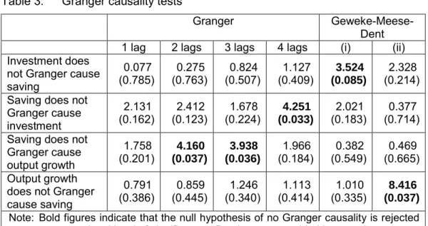
Empirical tests for Granger causality can be sensitive to the choice of lag length and the Granger and Geweke-Meese-Dent tests are performed for different lags. The Granger test is performed for lags 1 to 4. The Geweke-Meese-Dent test is performed for two different sets of lags: (i) including the dependent variable with two lags and the current independent variable, with two lags and one lead, and (ii) the dependent variable with four lags and the current independent variable, with four lags and two leads. Table 3 reports the results.
Table 3: Granger causality tests
Granger
Geweke-Meese-Dent
1 lag 2 lags 3 lags 4 lags (i) (ii)
Investment does not Granger cause saving
0.077
(0.785) (0.763)0.275 (0.507) 0.824 (0.409) 1.127 (0.085)3.524
2.328 (0.214) Saving does not
Granger cause investment
2.131
(0.162) (0.123)2.412 (0.224) 1.678 (0.033)4.251
2.021
(0.183) (0.714) 0.377 Saving does not
Granger cause output growth
1.758
(0.201) (0.037)4.160
3.938 (0.036)
1.966
(0.184) (0.549)0.382 (0.665) 0.469 Output growth
does not Granger cause saving
0.791
(0.386) (0.445)0.859 (0.340) 1.246 (0.414) 1.113 (0.335)1.010 (0.037)8.416
Note: Bold figures indicate that the null hypothesis of no Granger causality is rejected at conventional level of significance. P-values are provided in parentheses.
Table 3 shows that the direction of causation between saving and investment and saving and growth is ambiguous. The Granger test provides evidence that saving Granger causes investment and output growth. In contrast, the Geweke-Meese-Dent finds evidence of Granger causality from investment and output growth to saving.
Cross correlations between saving and investment and output growth, reported in Table 4, also show that there is no clear link between the variables.26 For example, the correlation between saving and past output growth is positive. This implies that higher output growth is followed by increased saving in future. However, the correlation between saving and future output growth is negative. This may be interpreted as households increasing their consumption (and hence lowering savings) in anticipation of higher output growth in future.
26 The cross correlation function of x and y is calculated using the following formula:
∑
∑
−∑
− − − = ρ − 2 t 2 t k t t y , x ) y y ( ) x x ( ) y y )( x x ( ) k ( .Table 4: Cross correlations
Saving (t)
Investment (t-4) -0.104
Investment (t-3) -0.056
Investment (t-2) 0.034
Investment (t-1) 0.381
Investment (t) 0.605
Investment (t+1) 0.600
Investment (t+2) 0.313
Investment (t+3) 0.042
Investment (t+4) -0.053
Output growth (t-4) 0.075
Output growth (t-3) 0.173
Output growth (t-2) 0.289
Output growth (t-1) 0.362
Output growth (t) 0.259
Output growth (t+1) -0.211
Output growth (t+2) -0.511
Output growth (t+3) -0.496
Output growth (t+4) -0.259
A three-variable VAR
To examine the dynamic inter-relationship between domestic saving, investment and real output growth, i.e. how does saving respond to an unforeseen increase in output growth, for example, we estimate a three-variable vector autoregression (VAR) model. A VAR is a system of equations, where each variable depends on its past realisations as well as the past realisations of all other variables in the system. Impulse responses of the VAR can then be used to examine the response of the variables in the system to particular shocks.
The vector representation of the VAR is given by
t 1 t
t c (L)x
x = +ϕ − +ε (4.3)
where x denotes the vector of variables in the model, i.e. saving, investment and real t output growth, c is a vector of constants, ϕ(L) is a pth degree matrix polynomial, and
t
ε is a vector of error terms.
To obtain the impulse responses, which trace out the response of the variables in the system to specific shocks, identifying restrictions need to be imposed. We impose the restriction that saving is exogenous and that real output growth is a function of past saving and investment rates.2728
27 The restriction implies a Choleski decomposition with the following ordering: saving, investment, real output growth. For a non-technical introduction to VARs see Buckle, Choy, Claus, Haugh and Szeto (2001).
28 Likelihood ratio tests at the 5 percent level chose a lag length of 2 to eliminate serial correlation from the residuals.
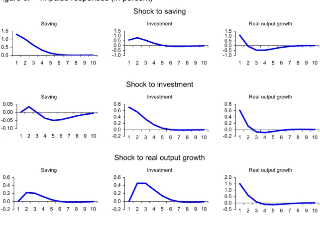
Figure 6: Impulse responses (in percent)
Shock to saving
Shock to investment
Shock to real output growth
Figure 6 plots the impulse responses of saving, investment and real output growth to shocks to each of the three variables in the system of one standard deviation in size. The horizontal axis denotes years. In line with time to build constraints, investment only increases gradually following a positive shock to saving and output growth. Following an unanticipated increase in saving, investment also rises, but by less than saving, while output growth, after initially increasing, actually declines. Output growth, after an initial rise, declines following higher saving because increased saving lowers domestic consumption and hence output growth. Saving rises following faster GDP growth. This finding is in line with other international empirical evidence (discussed further below). An unexpected temporary shock to investment increases real output growth. Following a positive shock to investment saving first increases and then declines. This may reflect higher household consumption (and lower saving) in anticipation of higher output growth.
Overall, the empirical results do not suggest any clear link between domestic saving, investment and real output growth in New Zealand although there is some evidence that higher real output growth produces greater saving. This is in line with international findings. Caroll and Weil (1994) examine the relationship between income growth and saving using both cross-country and household data. They find that (i) growth Granger causes saving, (ii) saving does not Granger cause growth, and (iii) households with higher income growth save more than households with predictably low income growth. Attanasio, Picci and Scorcu (2000) analyse the relationship between saving, investment and growth across 123 countries and find similar results.
Saving
0.0 0.5 1.0 1.5
1 2 3 4 5 6 7 8 9 10
Real output growth
-1.0 -0.50.0 0.5 1.0 1.5
1 2 3 4 5 6 7 8 9 10
Saving
-0.10 -0.05 0.00 0.05
1 2 3 4 5 6 7 8 9 10
Investment -0.2 0.0 0.2 0.4 0.6 0.8
1 2 3 4 5 6 7 8 9 10
Real output growth
-0.2 0.0 0.2 0.4 0.6 0.8
1 2 3 4 5 6 7 8 9 10
Investment -0.2 0.0 0.2 0.4 0.6
1 2 3 4 5 6 7 8 9 10
Real output growth
-0.5 0.0 0.5 1.0 1.5 2.0
1 2 3 4 5 6 7 8 9 10 Investment -1.0 -0.50.0 0.5 1.0 1.5
1 2 3 4 5 6 7 8 9 10
Saving -0.2 0.0 0.2 0.4 0.6
How mobile is capital in New Zealand?
Another indicator of whether or not domestic saving has been a constraining factor in New Zealand is capital mobility. Home bias in investors’ portfolios may be evidence that capital is not very mobile internationally and would support the claim that investment rates will depend on domestic saving rates. Investors can only diversify their portfolio through holding international assets if capital is mobile.
Figure 7: Proportion of New Zealand government bonds held for non-residents29
Source: Reserve Bank of New Zealand
As noted earlier home bias in investors’ portfolios appears to be less important for smaller countries. This seems to be the case for New Zealand. Home bias certainly appears to have declined for bonds. The proportion of New Zealand government bonds held for non-residents rose from around 10 percent in 1988 to around 40 percent currently, reaching a peak of 70 percent in September 1997 (see Figure 7). Recently, the proportion of government bonds held for non-residents declined, in part because of lower interest rates.
In the case of equities, the only data available are equity holdings by New Zealand households from the annual net wealth data constructed by the Reserve Bank of New Zealand. Figure 8 plots households’ domestic and foreign equity held directly and through managed funds from 1978 to 2000. It shows that the proportion of foreign equity held directly has fluctuated at around 11 percent. However, overall the share of foreign equity has been rising from about 17 percent in 1978 to about 52 percent in 2000 due to a steady increase in foreign equity held through managed funds. The proportion of equity held through managed funds has been rising following financial deregulation in the 1980s. The increase in managed funds foreign equity has been particularly marked, while the proportion of equity held directly has been falling.
29 Data from January 1993 to February 1994 exclude repurchase agreements.
0% 10% 20% 30% 40% 50% 60% 70% 80%
Figure 8: New Zealand household holdings of domestic and foreign equity
Source: Reserve Bank of New Zealand
New Zealand household portfolios are more diversified than in other OECD countries for which data are available (see Table 1) and may actually be close to optimally allocated. Estimates of “optimal diversification” suggest that the proportion of domestically held equity should be about equal to the ratio of nontradeable to total output. In 1999, the ratio of nontradeable output to gross domestic product was around 53 percent (see Easton 2001). This is close to the share of domestic equity in households’ portfolios (56 percent in 1999 and 48 percent in 2000).
Estimates of the share of foreign ownership in New Zealand companies also indicate that New Zealand portfolios are diversified. In 1997, about 35 percent of companies in New Zealand were publicly listed. Of these, only about 45 percent were domestically owned (see Day 1997).30 This suggests that capital flows freely into and out of New Zealand equity. A corollary is that investment and hence economic growth does not appear to have been constrained by domestic saving.
The supply of foreign funds determines the cost of borrowing and the cost of capital is another way to evaluate whether or not New Zealand has faced supply constraints. Lally (2000) compares the cost of real (adjusted for inflation) capital in New Zealand, Australia and the United States and finds that New Zealand’s real cost of capital is only modestly higher than Australia’s. However, the cost of real capital in New Zealand and Australia is considerably higher than in the United States. Higher costs in New Zealand and Australia than in the United States may be due to different firm size, book-to-market value and liquidity. Relatively high and persistent current account deficits may also contribute to higher cost of capital in Australia and New Zealand compared to the United States.
Hawkesby, Smith and Tether (2000) find similar results as Lally (2000). Over the 1990s, the risk premium in New Zealand’s interest rates versus interest rates in the
30 In 1997, foreigners owned 23 percent of the 65 percent privately owned companies. 0%
10% 20% 30% 40% 50% 60% 70% 80% 90% 100%
1978 1981 1984 1987 1990 1993 1996 1999 Direct holdings domestic
Managed funds holdings domestic Managed funds holdings overseas Direct holdings overseas
Domestic
United States was quite significant. However, the risk premium versus Australian interest rates was much smaller in magnitude.
The supply of venture capital also does not appear to be a significantly constraining factor for investment in New Zealand. Venture capital is a form of equity capital that is particularly suitable to the “financing of innovation” or financing of enterprises that are attempting to do something new.31 The venture capital market in New Zealand is evolving rapidly and the supply of capital has increased significantly over recent years, with the entry of new listed venture capitalists, large institutions, banks and corporate venture capital funds (see Infometrics Ltd 2000 and Perkins 2001). As a result, there is little evidence of a lack of venture capital for businesses (or a shortage of quality business propositions to invest in).
Long-run sustainability of the current account
Current and future supply of foreign capital in part depends on the sustainability of the current account or ability to repay external debt. A country’s current account deficit is sustainable in the long run if the solvency condition holds, i.e. if the present discounted value of future trade surpluses equals the current value of its external debt.
Evaluating New Zealand’s current account over the period June 1982 to September 1999, Kim, Buckle and Hall (2001) find that despite the substantial deterioration in the current account deficit during the late 1990s, movements in the current account as a whole have been consistent with the solvency condition. This result is based on statistical tests and an intertemporal optimisation model of the current account.32
Whether or not a country’s current account deficit will be sustainable in the future, i.e. whether or not future trade surpluses will be sufficient to maintain a stable debt to output ratio is subject to uncertainty and in part depends on the assumptions of the model used. As a result, a number of studies have attempted to identify a “checklist” of medium-term indicators that may signal an unsustainable current account position. These indicators generally include:
! the levels of domestic saving and investment
! economic growth
! openess of the economy
! composition of external liabilities
! financial structure
! monetary and exchange rate policy
! fiscal policy
! political stability
! perceptions of a country’s creditworthiness
31 The National Venture Capital Association defines venture capital as “patient risk equity capital invested in innovative and/or rapidly expanding enterprise”. It is “patient” capital as it tends to be relatively illiquid. Because of the relative illiquidity it is generally accompanied by clear exit strategies. Venture capital is an investment in real and intangible assets (a business), rather than a financial asset or instrument such as tradeable shares. Moreover, venture capitalists generally take an active interest in the business and are expected to offer more than simply money.
32 The optimisation model reflects the “permanent income hypothesis” of consumption and saving, where the private sector consumes the annuity value of its total discounted wealth
Little (2000) investigates indicators potentially relevant for New Zealand. He concludes that the checklist of indicators does not signal a long-run unsustainable position of the current account. The floating exchange rate regime, a strong financial sector and the composition of liabilities (discussed further below) all point to a strong underlying position of the New Zealand economy. Sound macroeconomic policies also make it unlikely that New Zealand will not be able to attract foreign capital in the future.
Figure 9: New Zealand’s current account and Standard and Poor’s Ratings Group foreign currency credit rating
Source: Statistics New Zealand, Standard and Poor’s Ratings Group and The Treasury
Figure 10: New Zealand’s current account and Moody’s Investors Service foreign currency credit rating
Source: Statistics New Zealand, Moody’s Investors Service and The Treasury
5 6 7 8 9 10
1983 1985 1987 1989 1991 1993 1995 1997 1999 2001 -10 -8 -6 -4 -2 0
Index of Standard and Poor's credit rating (left axis) Current account as a percentage of GDP (right axis)
20 21 22 23 24 25 26 27
1986 1988 1990 1992 1994 1996 1998 2000 -8 -7 -6 -5 -4 -3 -2 -1 0
Index of Moody's credit rating (left axis)
Moreover, despite relatively large current account deficits (see Figure 4), New Zealand’s credit rating has remained fairly stable. New Zealand’s current account as a percentage of GDP is plotted in Figure 9 with an index of Standard and Poor’s foreign currency credit rating for New Zealand and in Figure 10 with the equivalent index for Moody’s credit rating. The indices were constructed by assigning numbers from 1 to 10 from the lowest to highest rating for Standard and Poor’s and from 1 to 27 for Moody’s.33 Figures 9 and 10 show no obvious positive relationship between New Zealand’s current account deficit and its credit rating, which would point to an unsustainable current account deficit.
The composition of investment flows into New Zealand34
Using New Zealand’s International Investment Position statistics, total foreign investment can be divided into four main components: foreign direct investment, portfolio investment, government and other investment. Foreign direct investment (FDI) includes all capital transactions, both equity and debt, where a non-resident owns 25 percent or more of a New Zealand enterprise35. Portfolio investment mainly consists of non-resident purchases of government securities. It also includes other long-term bonds and corporate equities (not included in FDI) and non-resident holdings of other domestically issued securities. Government includes core central government capital transactions with non-residents (excluding changes in domestically issued securities and reserves). Other investment includes foreign exchange liabilities of banks, loans, currency, deposits and short-term bills and bonds.
Figure 11 plots the four components of foreign investment together with total foreign investment since the 1970s to 2000 (as a percentage of GDP). Over the period 1972 to 2000, total foreign investment has been fairly stable and fluctuated around 6 percent of GDP, moving in a range between 2 and 8 percent. However, the composition of foreign investment has changed significantly over time.
! Government
Up until the late 1980s, foreign investment inflows were dominated by government borrowing. However, in the 1990s the government began repaying its debt. This repayment appears as negative foreign investment in Figure 11.
! Foreign direct investment (FDI)
Government borrowing was largely replaced by foreign direct investment in the early to mid-1990s. FDI increased sharply from around 1-2 percent of GDP in the 1970s and 1980s to around 5 percent in the first half of the 1990s, before moderating to around 3 percent towards the end of the decade.
33 The appendix contains details on the ratings.
34 The discussion in this section is based on the International Monetary Fund’s Balance of Payments Manual 4 (BPM4) Statistics New Zealand data. Recently released BPM5 data are not incorporated. This is because data and methodological changes do not allow a direct comparison of the components of foreign investment flows. BPM5 international investment position data includes a new category: financial derivatives. Revised data are only available from June 2000 onwards. Some aggregates are comparable.
35 The ownership threshold was lowered to 10 percent in the quarterly Balance of Payments Manual 5 (BPM5) series.