AUSTRALIAN JOURNAL OF BASIC AND
Open Access Journal
Published BY AENSI Publication
© 2016 AENSI Publisher All rights reserved
This work is licensed under the Creative Commons Attribution International License (CC BY). http://creativecommons.org/licenses/by/4.0/
To Cite This Article: Huda, A. Rasheed and Zainab, N. Khalifa Function Using Different Priors. Aust. J. Basic & Appl. Sci.,
Bayes Estimators For The Maxwell Distribution U
Function Using Different Prior
1Huda, A. Rasheed and 2Zainab, N. Khalifa
1AL-Mustansiriyah University Collage of Science, Dept. of Math 2AL-Mustansiriyah University Collage of Science, Dept. of Math.
Address For Correspondence:
Huda, A. Rasheed, AL-Mustansiriyah University Collage of Science, Dept. of Math.
A R T I C L E I N F O
Article history:
Received 12 February 2016 Accepted 12 March 2016 Available online 20 March 2016
Keywords:
Maxwell distribution, Maximum likelihood, Bayes estimators, Jefferys prior, Gumbel type-II prior, Inverted Gamma prior, Inverted Levy prior, Quadratic loss function, Mean squared error.
Maxwell distribution was first introduced by J. C. Maxwell (1860) and then described by Boltzmann ( with a few assumptions.
Maxwell distribution plays an important role in Physics and chemistry. It gives the distribution of speeds of molecules in thermal equilibrium as given by statistical mechanics. For example, this distribution explains many fundamental gas properties in kinetic theory of gases, distributio
The Bayesian deduction requires appropriate choice of priors for the parameters. In the last several decades, Bayesian analysis focused on priors that are un
parameter, then it is better to make use of the informative priors. The parameters of the prior distribution called hyper-parameters.
Maxwell distribution (2008), and Maxwell
(2005) Bekker and Roux, studied empirical Bayes estimation for Maxwell distribution, and we have assumed that complete sample information is available, Sanku Dey
of a Maxwell distribution and obtain associated based on conjugate prior under scale invariant symmetric and a symmetric loss functions. Huda, A.
distribution under Quadratic loss function.
Model Description (Maxwell–Boltzmann, 2008; Maxwell distribution, 2008
The Maxwell (or Maxwell –
thermal equilibrium as given by statistical mechanics.
AUSTRALIAN JOURNAL OF BASIC AND
APPLIED SCIENCES
8414 -2309 : 8178 EISSN
-ISSN:1991
Journal home page: www.ajbasweb.com
© 2016 AENSI Publisher All rights reserved
This work is licensed under the Creative Commons Attribution International License (CC BY). http://creativecommons.org/licenses/by/4.0/
Huda, A. Rasheed and Zainab, N. Khalifa, Bayes Estimators For The Maxwell Distribution Under Quadratic Loss
Aust. J. Basic & Appl. Sci., 10(6): 97-103, 2016
timators For The Maxwell Distribution Under Quadratic Loss
sing Different Priors
Zainab, N. Khalifa
cience, Dept. of Math. Mustansiriyah University Collage of Science, Dept. of Math.
Mustansiriyah University Collage of Science, Dept. of Math.
A B S T R A C T
For estimating an unknown parameter for the Maxwell distribution, we obtained some Bayes estimators under Quadratic loss function using Non
represented by Jefferys prior and Informative priors as Gumbel
(Inverted Gamma and Inverted Levy) priors. All these estimators compared with Maximum likelihood estimator. According to Monte-Carlo simulation study, the performance of these estimates is compared depending on the mean squared error (MSE’s) and reached to, the Bayes estimator under Inverted Gamma prior is the best estimator, comparing to other priors.
INTRODUCTION
Maxwell distribution was first introduced by J. C. Maxwell (1860) and then described by Boltzmann (
Maxwell distribution plays an important role in Physics and chemistry. It gives the distribution of speeds of molecules in thermal equilibrium as given by statistical mechanics. For example, this distribution explains many
erties in kinetic theory of gases, distribution of energies and moments,…etc
The Bayesian deduction requires appropriate choice of priors for the parameters. In the last several decades, analysis focused on priors that are un-informative. But if we have enough information about the parameter, then it is better to make use of the informative priors. The parameters of the prior distribution
(2008), and Maxwell-Boltzmann (2008) are giving a summary of this applications. In (2005) Bekker and Roux, studied empirical Bayes estimation for Maxwell distribution, and we have assumed mation is available, Sanku Dey (2011) studies on Bayes estimators of the parameter of a Maxwell distribution and obtain associated based on conjugate prior under scale invariant symmetric and a Rashed (2013) derived Minimax estimation of the parameter of the Maxwell distribution under Quadratic loss function.
Boltzmann, 2008; Maxwell distribution, 2008):
Boltzmann) distribution gives the distribution of speeds of molecule thermal equilibrium as given by statistical mechanics.
Estimators For The Maxwell Distribution Under Quadratic Loss
nder Quadratic Loss
For estimating an unknown parameter for the Maxwell distribution, we obtained some Bayes estimators under Quadratic loss function using Non-informative prior, represented by Jefferys prior and Informative priors as Gumbel Type II and Conjugate (Inverted Gamma and Inverted Levy) priors. All these estimators compared with Carlo simulation study, the performance of these estimates is compared depending on the mean squared errors (MSE’s) and reached to, the Bayes estimator under Inverted Gamma prior is the best
Maxwell distribution was first introduced by J. C. Maxwell (1860) and then described by Boltzmann (1870)
Maxwell distribution plays an important role in Physics and chemistry. It gives the distribution of speeds of molecules in thermal equilibrium as given by statistical mechanics. For example, this distribution explains many
n of energies and moments,…etc.
The Bayesian deduction requires appropriate choice of priors for the parameters. In the last several decades, informative. But if we have enough information about the parameter, then it is better to make use of the informative priors. The parameters of the prior distribution are
(2008) are giving a summary of this applications. In (2005) Bekker and Roux, studied empirical Bayes estimation for Maxwell distribution, and we have assumed ies on Bayes estimators of the parameter of a Maxwell distribution and obtain associated based on conjugate prior under scale invariant symmetric and a estimation of the parameter of the Maxwell
Defining = , where K is the Maxwell constant, T is temperature, m is the mass of a molecule. The probability density function and the cumulative distribution function of Maxwell distribution over the rang x∈ 0,∞ are given by :
f( | =
√ ̸ ; 0 < X, θ (1)
F(x)= Γ( , ) (2)
Where Γ(x ,α)= " !#∝ %# is the incomplete gamma function (Krishna Hare and Malik Manish, 2008).
It can also be expressed as follows
F(x; = 2 '( )
√ * −√
Where '( =
√ ,
∞
" dw ,is the error function.
Properties of Maxwell distribution[7]:
We can summarize the most important properties by the following points: 1- The nth row moment is:
-́/=√ 0 )/1 *
2
; 4 > −3 So that:
If n = 1 ,then -́ = 27 , and if n=2 ,then -́ = 37 ;..., etc.
2- Mean=27
3- Variance = 38 − 8
4- Mode = √
5- Median= :;% + 2 : =4
= 7 √8+4)
=1.0856√8
6- R(t)=P(x>t)=
√ ∞
> %
=
√ ? @, 2, ; @ > 0
Where ? @, 2, = >∞ A ,B C, , is the Jacobian function
7- ℎ @ =E > F > =
> GHI J >, ,
Estimation of Parameter:
In this section we can used two methods to estimation parameter
1.Maximum likelihood estimation (Rasheed, H.A., 2013):
We introduce the concept of maximum likelihood estimation with Maxwell distribution. Let n items have
an independent and identically distributed, then the likelihood of the sample from Maxwell distribution with parameter is given by:
K L M; N = 8MO / ( M; = )√ *
/
2(8MO/ M)
∑2QR Q
From which we calculate the log-likelihood function:
S4K M; = 4S4 )√ * + ln 1 − /S4 + 2 ∑ S4 M−∑ Q
2 QR
/
MO (3)
Now, differentiating partially equation(3)with respect to : WX/Y Q;
W =
/+∑2QR Q
(4)
θZ[\O ∑2QR/ Q = /, where T=∑/MO M (5)
2. Bayes Estimators:
Let ]^, ]_, … , ]a be a random sample of size n with probability density function given in equation (1) and likelihood function given in equation (5), then, the Bayes estimators of the parameter b under different prior distributions which is mentioned below, can be obtained as follows:
2.1. Jefferys Prior Information (Al-Baldawi, T., H.K, 2013):
Assume that, the unknown scale parameter has no-information prior density defined as using Jefferys prior information c which is derived to be
c ∝ de (6)
Where e = −4f )W X/ E ;
W * is the Fisher's information matrix. Hence,
c = g7−4f )W hi E ;j,W * (7)
With k is a constant.
By taking the logarithm for distribution and taking the partial derivative with respect to , we get:
k S4 ( |
k = −2 +3
k S4 ( |
k =2 −3 2
f lk S4 ( |k m = f n 2 o − f l3 2 m
= − f = (8)
After Substitution (8) into(6), we get
c = g7−4 )− * =p7 / (9)
Now, combining the prior 9 with the likelihood function 5 , we have the posterior distribution of θ with Jefferys prior information which is given by :
ℎ L | N = c K ; … … . . /
c∞
" K ; … … . . / %
ℎ L | N = 2t G ul
∑2QR m
2t ∞
v G ul ∑2QR mC
(10)
On Simplification ,we have
ℎ L | N =L∑2QR N
2
GH∑2QR ⁄
2t x 2 =
2
GHy
) 2t * x 2 (11)
This posterior density is recognized as the density of the Inverse Gamma distribution, i.e.: θ|x ~IG ( /, |
Where , E(θ|x)= 2 , Var (θ|x
) 2 * )2 * , n > 1
2.2. Gumbel Type II Prior Information:
Using Gumbel type II prior with hyper parameter (b), which is defined as (Ali, S., et al., 2012; Rasheed, H.A. and E.F. Ai-Shareefi, 2015),
g θ = b )θ* Exp •θ‚ƒ b,θ> 0 (12)
ℎ L | N = ( 2t ) G
HL∑2QR t…N/
( 2t ) G
H)∑2QR t…*/ C
∞
v
(13)
After simplification, we get:
ℎ L | N =L∑2QR 1‡N2t GHL∑Š‹R ˆ t‰N/θ
( 2t )Γ( Š1 ) =
( 1‡)2t GH(yt…)
( 2t )Γ)Š1 * (14)
This posterior is recognized as the density of the Inverse Gamma distribution, i.e.: θ|x~IG ( i+ 1, Ž + •)
Where, ELθ|xN = •1‚Š , VarLθ|xN = ( 1‡)
) Š* )Š * , 4 > 1
2.3. Inverted Gamma Prior information (Al-Baldawi, T., H.K, 2015):
This conjugate prior distribution is the distribution of the reciprocal of a variable distributed according to Gamma distribution that is assumed to be:
c ( ) =”Γ–• •t ”⁄ , —, ˜, >0 (15)
With scale parameter — and shape parameter ˜.
The posterior distribution under the assumption of gamma prior is:
ℎ ( | ) = ( 2t•t )
G u L∑2QR t™N
( 2t•t )
∞
v š›œ )∑ t™
2
QR * C (16)
On Simplification , we have:
ℎ L | N =L∑2QR 1”N2t• GH(∑2QR t™)⁄
( 2t•t ) x( 2t•) =
( 1”) 2 GH(yt™)
( 2t•t ) x( 2t•) (17)
This posterior density is recognized as the density of the Inverse Gamma distribution:θ|x~IG ( /+ ˜ , | +
—)
Where, E(θ|x) = 21”
1– , Var (θ|x) =
( 1”)
) 21– * ) 21– * , n > 1
2.4. Inverted Levy Prior Information:
The inverted Levy prior is assumed to be (Sindhu, T.N., M. Aslam, 2013)
c ( ) = 7• √ ž , Ÿ > 0 (18)
Where Ÿ is the hyper parameter.
The posterior distribution of is given by:
ℎ L | N = ( 2t ) G u
∑2QR t ž ¡
( 2t )
∞
v G u ∑2QR t ž¡C
(19)
On Simplification, we have
ℎ L | N =)∑2QR 1ž* 2H
GH(∑2QR tž)¢
( 2t ) x( 2H ) =
( 1ž) 2 GH(ytž)
( 2t ) x( 2H ) (20)
Notice that, ℎ L | N is recognized as the density of the Inverse Gamma distribution, namely, θ|x~IG
( /− , | +•)
Where, E(θ|x) = 1
ž
( 2 ) , Var (θ|x) = ) 1ž* )2 * )2 £*
2.5. Bayes Estimator Under Quadratic Loss Function:
De Groote (1970) discussed different types of loss function and obtained the Bayes estimates under these loss function which is a non- negative symmetric and continuous loss function [4],[8] and is defined as :
R§Lθ,¥ θN = E )1 −θθZ* (22)
= )1 −θZ θ* ∞
" h Lθ|xNdθ
∂R§Lθ,¥ θN
∂θZ = 2 ª l1 −
θZ θm n−
1
θo h Lθ|xNdθ ∞
"
Let -®¯Lθ,¥ θN
-θZ = 0, yields:
⇒θZ θ ∞
" h Lθ|xNdθ− θ ∞
" h Lθ|xNdθ= 0
Hence, Bayes estimator under the Quadratic loss function will be:
θZ§=± (θ| )
±(
θ | )
(23)
(²) ³ith Jefferys prior information:
According to the posterior density function (11), the Bayes estimator of θof Maxwell distribution under Quadratic loss function is obtained by applying (23) as follows:
E n1
θ´| o = ª
1
θ´ ∞
"
h Lθ|xNdθ
= θµ L∑ › Š
‹R N
Š
Γ)Š* θ( Št ) ∞
" e
H ∑Š‹R ˆ
θ dθ
Hence,
E )θµ| * =
Γ(21 )
Γ)2*L∑2QR N¶ , · = 0, 1, 2, … (24)
After substituting, we get the Bayes estimator of parameter under Quadratic loss function with Jefferys prior information as follows:
Z¸J=∑2QR
( 21 ) (25)
(¹¹) With Gumbel Type -II prior information:
Based on the posterior density function (14), the Bayes estimator of º of Maxwell distribution under Quadratic loss function is obtained as:
f n 1 | o = ª1
∞
"
ℎ L | N%
= ¶ L∑ 1‡
2
QR N2t
Γ) 21 * ( 2t )
∞
"
H(∑2QR t…)
%
Hence,
f ) ¶| * =
Γ( 21 1 )
Γ( 21 )(∑2QR 1‡)¶ (26)
After substituting, we get the Bayes estimator of parameter θ under Quadratic loss function with Gumbel Type- II information as:
Z¸»Y=(∑2QR 1‡)
21 (27)
(iii) With Inverted Gamma Prior Information:
From (17) posterior density function, the Bayes estimator of º of Maxwell distribution under Quadratic loss function is obtained as:
E )θµ| * = θµ
∞
" h Lθ|xNdθ
= ¶ L∑ 1” 2
QR N2t•
Γ)21–* ( 2t•t ) ∞
"
H(∑2QR t™)
%
Hence, E )
θµ| * =
Γ( 21 1–)
Z¸»¼=(∑2QR 1”)
( 21–1 ) (29)
(V) With Inverted Levy Prior Information:
From (20) posterior density function, the Bayes estimator of º of Maxwell distribution under Quadratic loss function is obtained as:
E nθ1´| o = ªθ1´
∞
"
h Lθ|xNdθ
= ª 1
∞
"
)∑/ + Ÿ2
MO *
/
/
Γ(342 −12)
(∑2QR 1•)
%
Hence,
E )θµ| * =
Γ( 21 )
Γ(2 ))∑2QR 1ž*¶ , · = 0, 1, 2, …
(30)
After substituting ,we get the Bayes estimator of parameter b under Quadratic loss function with Inverted Levy prior information as follows:
Z¸½Y=(∑2QR 1ž)
( 21 ) (31)
4. Simulation Study:
Mean Squared Errors (MSE’s), are considered to compare the different estimators of the parameter θ that obtained by the method of Maximum likelihood and Bayes Estimators for Quadratic Loss function methods. In this simulation study, the number of replication used was I = 5000 samples of sizes n = 5,10, 20, 50, 100 from the Maxwell distribution with different values of θ where, θ = 0.5, 1.5, 3.
In this section, Monte-Carlo simulation study is performed to compare the methods of estimation by using
mean squared errors (MSE’s) as an index for precision to compare the efficiency of each of estimators, where:
MSE( ) = ∑¾QRL¥½Q N
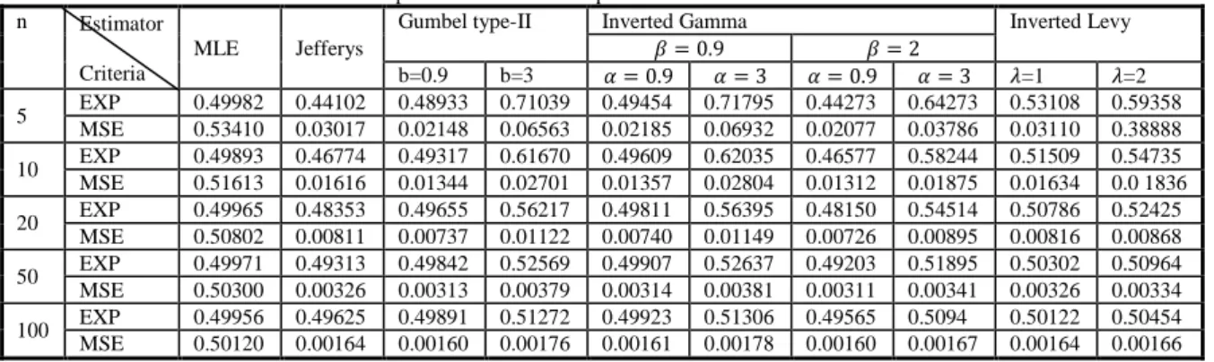
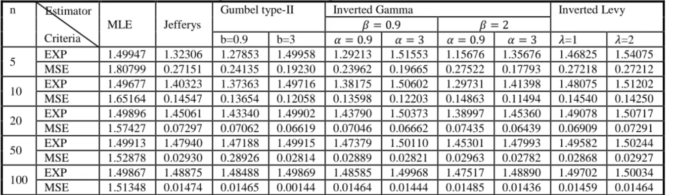
The results are summarized and tabulated in tables (1-3) which contain the expected values and (MSE's) for estimating the scale parameter θ. and we have observed that:
1- Table (1), shows that, the performance of Bayes estimator under Inverse Gamma prior when (θ=
0.5) and (α= 0.9 and β= 2) is the best estimator.
2- Table (2), shows that ,the performance of Bayes estimator under Inverted Gamma prior when (θ=
1.5) and (α= 3 and β= 2) is the best estimator.
3- Table(3), shows that ,the performance of Bayes estimator under Inverted Gamma prior when ( = 3) and (— = 3 and ˜=0.9) is the best estimator.
4- For all parameter values, an obvious that, reduction in (MSE) is observed with the increase in all sample sizes. Finally ,It is observed that, (MSE) of all estimators of the scale parameter is increasing with the increase of the scale parameter value with all sample sizes.
Generally, the comparison results showed that, the performance of Bayes estimator under Quadratic loss functions based on Inverted Gamma prior is more appropriate than using other priors, on condition that, the ratio between the scale parameter — to the location parameter ˜ is nearly, equivalent to the estimated parameter .
Table 1: Estimates and MSEs under different priors for different sample sizes with =0.5 n Estimator
Criteria
MLE Jefferys
Gumbel type-II Inverted Gamma Inverted Levy
˜ = 0.9 ˜ = 2
b=0.9 b=3 — = 0.9 — = 3 — = 0.9 — = 3 Ÿ=1 Ÿ=2
5 EXP 0.49982 0.44102 0.48933 0.71039 0.49454 0.71795 0.44273 0.64273 0.53108 0.59358 MSE 0.53410 0.03017 0.02148 0.06563 0.02185 0.06932 0.02077 0.03786 0.03110 0.38888 10 EXP 0.49893 0.46774 0.49317 0.61670 0.49609 0.62035 0.46577 0.58244 0.51509 0.54735 MSE 0.51613 0.01616 0.01344 0.02701 0.01357 0.02804 0.01312 0.01875 0.01634 0.0 1836 20 EXP 0.49965 0.48353 0.49655 0.56217 0.49811 0.56395 0.48150 0.54514 0.50786 0.52425
Table 2: Estimates and MSEs under different priors for different sample sizes with =1.5 n Estimator
Criteria
MLE Jefferys
Gumbel type-II Inverted Gamma Inverted Levy
˜ = 0.9 ˜ = 2
b=0.9 b=3 — = 0.9 — = 3 — = 0.9 — = 3 Ÿ=1 Ÿ=2 5 EXP 1.49947 1.32306 1.27853 1.49958 1.29213 1.51553 1.15676 1.35676 1.46825 1.54075
MSE 1.80799 0.27151 0.24135 0.19230 0.23962 0.19665 0.27522 0.17793 0.27218 0.27212 10 EXP 1.49677 1.40323 1.37363 1.49716 1.38175 1.50602 1.29731 1.41398 1.48075 1.51202 MSE 1.65164 0.14547 0.13654 0.12058 0.13598 0.12203 0.14863 0.11494 0.14540 0.14250 20 EXP 1.49896 1.45061 1.43340 1.49902 1.43790 1.50373 1.38997 1.45360 1.49078 1.50717 MSE 1.57427 0.07297 0.07062 0.06619 0.07046 0.06662 0.07435 0.06439 0.06909 0.07291 50 EXP 1.49913 1.47940 1.47188 1.49915 1.47379 1.50110 1.45301 1.47993 1.49582 1.50244 MSE 1.52878 0.02930 0.28926 0.02814 0.02889 0.02821 0.02963 0.02782 0.02868 0.02927 100 EXP 1.49867 1.48875 1.48488 1.49869 1.48585 1.49968 1.47517 1.48890 1.49702 1.50034 MSE 1.51348 0.01474 0.01465 0.00144 0.01464 0.01444 0.01485 0.01436 0.01459 0.01464
Table 3: Estimates and MSEs under different priors for different sample sizes with =3 n Estimator
Criteria
MLE Jefferys
Gumbel type-II Inverted Gamma Inverted Levy
˜ = 0.9 ˜ = 2
b=0.9 b=3 — = 0.9 — = 3 — = 0.9 — = 3 Ÿ=1 Ÿ=2
5 EXP 2.99894 2.64613 2.46232 2.68337 2.48852 2.71192 2.22782 2.42781 2.87401 2.93651 MSE 4.23306 1.08605 1.05829 0.86944 1.04726 0.86863 1.22593 0.95705 1.10055 1.08871 10 EXP 2.99355 2.80645 2.69431 2.81784 2.71025 2.83451 2.54463 2.66129 2.92924 2.96150 MSE 3.61303 0.58190 0.57572 0.51545 2.71025 0.51538 0.63754 0.54490 0.58514 0.58161 20 EXP 2.99792 2.90121 2.83868 0.27392 2.84757 2.91340 2.75266 2.81630 0.29265 2.98156 MSE 3.29916 0.29187 0.29078 2.95933 0.28965 0.27392 0.31013 0.28270 0.29265 0.29178 50 EXP 2.99825 2.95880 2.93206 2.95933 2.93588 2.96318 2.89447 2.92140 2.98502 2.99164 MSE 3.11688 0.11722 0.11716 0.11419 0.11695 0.11419 0.12081 0.11585 0.11728 0.11713 100 EXP 2.99735 2.97750 2.96383 2.97765 2.96578 2.97961 2.94446 2.95818 2.99072 2.99404 MSE 3.05659 0.05896 0.05995 0.05819 0.05893 0.05818 0.06002 0.05868 0.05893 0.05888
REFERENCES
Ali, S., M. Aslam, N.Abbas and S.M. Ali Kazmiz, 2012. "Scale Parameter Estimation of the Laplace Modeling using Different Loss Function ", International Journal of the statistics and Probability, 1(1):105-127.
Al-Baldawi, T., H.K, 2013. "Comparison of Maximum Likelihood and Some Bayes Estimators for Maxwell Distribution based on non-informative Priors", Baghdad Science Journal, 10(2).
Al-Baldawi, T., H.K, 2015. " Some Bayes Estimators for Maxwell Distribution with Conjugate Information Priors", Al-Mustansiriyah Journal of Science, 26: 1.
Dey, S., 2008. "Minimax estimation of the scale parameter of Rayleigh distribution under Quadratic loss function ",Data Science Journal, 7: 23-30.
Krishna Hare and Malik Manish, 2008. "Reliability estimation in Maxwell distribution with type –II censored data ",International Journal of Quality &Reliability Management (USA), 26(3): 182-195.
Maxwell–Boltzmann, 2008. ,available at: http://Wikipedia.org/wiki/Maxwell-Boltzmann distribution (accessed June 20.2008).
Maxwell distribution, 2008, available at: http://math world.Wolfram.com/Maxwell distribution html(accessed June 20.2008).
Makhdoom, I., 2011. "Minimax estimation of the parameter of the generalized Exponential distribution ",International Journal of academic research, 2(2): 515-527.
Rasheed, H.A. and E.F. Ai-Shareefi, 2015. "Minimax Estimation of the Scale Parameter of Laplace Distribution under Different Loss Function". International Journal of Emerging Technologies in Computational and Applied Sciences, 14(1): 01-09.
Rasheed, H.A., 2013."Minimax Estimation of The Parameter of the Maxwell Distribution under Quadratic loss function", Journal of Al-Rafidain University College, ISSN(1681-6870), Issue No.31.
Sanku Dey, 2011. "Bayes estimation and prediction for Maxwell distribution st.Anthony,s College , Shilong, Meghalaya, India.
Sindhu, T.N., M. Aslam, 2013. "Bayesian estimation on the proportional inverse Weibul distribution under different loss functions". Advances in Agriculture, Science and Engineering Research, 3(2): 641-655.