Research Article An Approach to Semantic and Structural Features Learning for Software Defect Prediction

Research Article

An Approach to Semantic and Structural Features Learning for

Software Defect Prediction

Shi Meilong,

Peng He ,

Haitao Xiao,

Huixin Li,

and Cheng Zeng

Correspondence should be addressed to Peng He; [email protected]

Received 20 December 2019; Revised 1 February 2020; Accepted 24 February 2020; Published 6 April 2020

Guest Editor: Chunlai Chai

Copyright © 2020 Shi Meilong et al. This is an open access article distributed under the Creative Commons Attribution License, which permits unrestricted use, distribution, and reproduction in any medium, provided the original work is properly cited. Research on software defect prediction has achieved great success at modeling predictors. To build more accurate predictors, a number of hand-crafted features are proposed, such as static code features, process features, and social network features. Few models, however, consider the semantic and structural features of programs. Understanding the context information of source code files could explain a lot about the cause of defects in software. In this paper, we leverage representation learning for semantic and structural features generation. Specifically, we first extract token vectors of code files based on the Abstract Syntax Trees (ASTs) and then feed the token vectors into Convolutional Neural Network (CNN) to automatically learn semantic features. Meanwhile, we also construct a complex network model based on the dependencies between code files, namely, software network (SN). After that, to learn the structural features, we apply the network embedding method to the resulting SN. Finally, we build a novel software defect prediction model based on the learned semantic and structural features (SDP-S2S). We evaluated our method on 6 projects collected from public PROMISE repositories. The results suggest that the contribution of structural features extracted from software network is prominent, and when combined with semantic features, the results seem to be better. In addition, compared with the traditional hand-crafted features, theF-measure values of SDP-S2S are generally increased, with a maximum growth rate of 99.5%. We also explore the parameter sensitivity in the learning process of semantic and structural features and provide guidance for the optimization of predictors.

1. Introduction

Software defect is an error in the code or incorrect behavior in software execution, also defined as failure to meet intended or specified requirements. Software reliability is regarded as one of the crucial problems in software engi-neering. Thus, the models used to ensure software quality are required, and the software defect prediction model is one of them. Defect prediction can estimate the most defect-prone software components precisely and help developers allocate limited resources to those bits of the systems that are most likely to contain defects in testing and maintenance phases [1].

As we all know, in software life cycle, the earlier you find the defect, the less it costs to fix [2]. Therefore, how to detect defects quickly and accurately is always an open challenge in

the field of software engineering and has attracted extensive attention from industry and academia.

Typical defect prediction is composed of two parts: features extraction from source files and classifiers con-struction using various machine learning algorithms. Existing methods are dominated by traditional hand-crafted features, namely, source code metrics (e.g., CK, Halstead, MOOD, and McCabe’s CC metrics). Unfortunately, these metrics generally overlook some important information implied in the code, such as semantic and structural in-formation. Meanwhile, extensive machine learning algo-rithms have been adopted for software defect prediction, including Support Vector Machine (SVM), Na¨ıve Bayes (NB), Decision Tree (DT), etc.

Programs have well-defined syntax and rich semantics hidden in the Abstract Syntax Trees (ASTs), which have been Volume 2020, Article ID 6038619, 13 pages

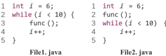
successfully used for programming patterns mining [3, 4], code completion [5, 6], and code plagiarism detection [7]. For example, Figure 1 shows two Java files, both of which contain an assignment statement, a while statement, a function call, and an increment statement. If we use tra-ditional features to represent these two files, they are identical because of the same source code characteristics in terms of lines of code, function calls, raw programming tokens, etc. However, they are actually quite different according to semantic information. In other words, semantic information as new discriminative features should also be useful for characterizing defects for improving defect prediction.

At present, deep learning has emerged as a powerful technique for automated feature generation, since deep learning architecture can effectively capture highly com-plicated nonlinear features. To make use of its powerful feature generation ability, some researchers [8, 9] have al-ready leveraged deep learning algorithms, such as Deep Belief Network (DBN) and Convolutional Neural Network (CNN) in learning semantic features from programs’ ASTs, and verified that it outperforms traditional hand-crafted features in defect prediction.

As demonstrated by researchers [9], CNN is superior to DBN because of CNN’s powerful efficiency to capture local patterns. Hence, CNN is capable of detecting local patterns and then conducting defect prediction. Since slight differ-ence in local code structure, such as the code order differdiffer-ence illustrated in Figure 1, may trigger huge variance in the global program, we apply CNN instead of DBN to the construction of the defect prediction model.

However, the abovementioned studies still overlook the globally structural information among program files which can lead to more accurate defect prediction, although they consider the fine-grained semantic information in the program files. In order to better represent the global structure of software, previous studies [10–12] have suc-cessfully abstracted a software as a directed dependency network using complex network theory, usually termed as software network (SN), where software components such as files, classes, or packages are nodes and the dependency relationships between them are edges. Furthermore, using network analysis technologies, they have demonstrated the effectiveness of network structure information in improving the performance of defect prediction.

Unfortunately, network features the above authors used in defect prediction modeling, such as modularity, cen-trality, and node degree, still belong to the traditional hand-crafted features. As an emerging deep learning technology, network representation learning becomes a novel approach for automatically learning latent features of nodes in a network [13] and receives much attention. Therefore, using representation learning to extract the structural information from code files and further apply the learned features to defect prediction may effectively improve the performance of existing prediction models.

Unlike the existing studies, in our work, instead of using traditional hand-crafted metrics, we introduced deep learning technologies to automatically extract the semantic

(local fine-grained) and structural (global coarse-grained) features of code files for defect prediction modeling and seek empirical evidence that they can achieve acceptable per-formance compared with the benchmark models. Our contributions to the current state of research are summa-rized as follows:

(i) We further demonstrated that the automatically learned semantic features can significantly improve defect prediction compared to traditional features (ii) In terms of improving the performance of defect

prediction, we also validated that the contribution of structural features extracted from software net-work by representation learning is comparable to that of semantic features on the whole

(iii) Interestingly, we also found that the combination of semantic and structural features has greater impact on the improvement of prediction performance The rest of this paper is organized as follows. Section 2 is a review of related work on this topic. Sections 3 and 4 describe the preliminary theories and the approach of our empirical study, respectively. Section 5 is the detailed ex-perimental setups and the primary results. Some threats to validity that could affect our study are presented in Section 6. Finally, Section 7 concludes the work and presents the agenda for future work.

2. Related Studies

2.1. Software Defect Prediction. Software defect prediction technology has been widely used in software quality as-surance and can effectively reduce the cost of software development. It uses the previous defect data to build a predictor and then employs the established model to predict whether a new code fragment is defective. At present, conventional software defect prediction can be roughly divided into two steps. The first stage is feature extraction, which makes the representation of defects more efficient by manually designing some features or combining existing features. The second is the classification by machine learning methods, specifically, by using the learning algorithm to establish an accurate model, so as to provide better prediction.

Most defect prediction techniques leverage features that are composed of the hand-crafted code metrics to train machine learning-based classifiers [14]. Commonly used code metrics include static code metrics and process metrics. The former include McCabe metrics [15], CK metrics [16], and MOOD metrics [17], which are widely examined and used for defect prediction. Compared to the above static

code metrics, process metrics can reveal much about how programmers collaborate on tasks. Moser et al. [18] used the number of revisions, authors, past fixes, and ages of files as metrics to predict defects. Nagappan and Ball [19] proposed code churn metrics and showed that these features were effective for defect prediction. Hassan [20] used entropy of change features to predict defects. Other process metrics, including developer individual characteristics [21] and collaboration between developers [22, 23], were also useful for defect prediction.

Meanwhile, many machine learning algorithms have been adopted for defect prediction, including Support Vector Machine (SVM) [24], Bayesian Belief Network [25], Naive Bayes (NB) [26], Decision Table (DT) [1], neural network [27], and ensemble learning [28]. For instance, Kumar and Singh [24] evaluated the capability of SVM with combinations of different feature selection and extraction techniques in predicting defective software modules and tested on five NASA datasets. In [25], the authors predicted the quality of a software by using the Bayesian Belief Net-work. Arar and Ayan [26] proposed a Feature Dependent Naive Bayes (FDNB) classification method to software defect prediction and evaluated their approach on PROMISE datasets. He et al. [1] examined the performance of tree-based machine learning algorithms on defect prediction from the perspective of simplifying metric. Li et al. [28] proposed a novel Two-Stage Ensemble Learning (TSEL) approach to defect prediction using heterogeneous data. They experimented on 30 public projects and showed that the proposed TSEL approach outperforms a range of competing methods.

In addition, to overcome the lack of training data, a cross-project defect prediction (CPDP) model was proposed by some research studies. To improve the performance of CPDP, Turhan et al. [29] proposed to use a nearest-neighbor filter for target project to select training data. Nam et al. [30] proposed TCA+, which adopted a state-of-the-art technique called Transfer Component Analysis (TCA) and optimized normalization process. They evaluated TCA+ on eight open-source projects, and the results showed that TCA+ signifi-cantly improved CPDP. Nam et al. [21] also presented methods for defect prediction that match up different metrics in different projects to address the heterogeneous data problem in CPDP.

2.2. Deep Learning in Software Engineering.

Representation learning has been widely applied to feature learning, which can capture the highly complex nonlinear information. Recently, deep learning algorithms have been adopted to improve research tasks in software engineering. Yang et al. [31] proposed an approach to generate features from existing features by using Deep Belief Network (DBN) and then used these new features to predict whether a commit is buggy or not. This work was motivated by the weaknesses of Logistic Regression (LR) that LR cannot combine features to generate new features. They used DBN to generate features from 14 traditional features and several developer experience-related features. Wang et al. [8] also

leveraged DBN to automatically learn semantic features from token vectors extracted from programs’ Abstract Syntax Trees (ASTs) and further validated that the learned semantic features significantly improve the performance of defect prediction. Similarly, Li et al. [9] used convolution neural network for feature generation based on the pro-gram’s AST and proposed a framework of defect prediction. To explore program’s semantics, Phan et al. [32] attempted to learn new defect features from program control flow graphs by convolution neural network.

However, these studies still ignore the structural features of programs, such as the dependencies between program files. Prior studies [12, 33–35] have demonstrated the ef-fectiveness of network structure information in improving the performance of the defect prediction model. Nowadays, the node of a network can be represented as a low-di-mensional vector by means of network embedding. A large number of network embedding algorithms have been suc-cessfully applied in network representational learning, in-cluding DeepWalk [36], Node2vec [37], and LINE [38]. Through the representational learning of software networks formed by various dependencies between code files, in this paper, we extract structural features of program files, so as to supplement the existing semantic features for defect prediction.

2.3. Software Network. In recent years, software networks (SN) have been widely utilized to characterize the problems in software engineering practices [39]. For example, some complexity metrics based on software networks are posed to evaluate the software quality. Gu et al. [40] pro-posed a metric of cohesion based on SN for measuring connectivity of class members. From the perspective of social network analysis (SNA), Zhang et al. [41] put forward a suite of metrics for static structural complexity, which overcomes the limitations of traditional OO software met-rics. Ma et al. [42] proposed a hierarchical set of metrics in terms of coupling and cohesion and analyzed a sample of 12 open-source OO software systems to empirically validate the set. Pan and Chai [43] leverage a meaningful metric based on SN to measure software stability.

In addition to complexity metrics, software network-based measures for stability and evolvability have also been presented by some researchers. Zhang et al. [41] analyzed the evolution of software networks from several kinds of object-oriented software systems and discovered some evolution rules such as distance among nodes increase and scale-free property. Gu and Chen [44] validated software evolution laws using network measures and discussed the feasibility of modeling software evolution. Peng et al. [11] constructed the software network model from a multigranularity perspective and further analyzed the evolutions of three open-source software systems in terms of network scale, quality, and structure control indicators, using complex network theory. Besides, for software ranking task, Srinivasan et al. [45] proposed a software ranking model based on software core components. Pan et al. constructed [46] a novel model ElementRank based on SN, which leverages multilayer

complex network to rank software. In addition, SN is also applied to analyze the structure of software structure [47]. Furthermore, a generalized k-core decomposition model [48] is leveraged to identify key class.

3. Preliminaries

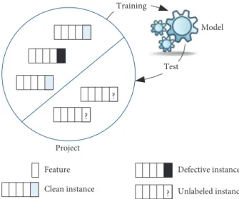
3.1. Overview of Software Defect Prediction. Software defect prediction plays an important role in reducing the cost of software development and ensuring the quality of software. It can find the possible defective code blocks according to the features of historical data, thus allowing workers to focus their limited resources on the defect-prone code. Figure 2 presents a basic framework of software defect prediction and has been widely used in existing studies [1, 8, 12, 18, 19, 24, 25].

Most defect prediction models are based on machine learning; therefore, it is a first step to collect defect datasets. The defect datasets consist of various code features and labels. Commonly used features are various software code metrics mentioned above. Label indicates whether the code file is defective or not for binary classification. In the setting, predictor is trained using the labeled instances of project and then used to predict unlabeled (“?”) instances as defective or clean. In the process of defect prediction, the instances used to learn classifier is called training set and the instances used to evaluate classifier are called test set.

3.2. Convolutional Neural Network. Convolutional neural network (CNN) is one of the most popular algorithms for deep learning, a specialized kind of neural networks for processing data that have a known gridlike topology [49]. Compared with traditional artificial neural network, CNN has many advantages and has been successfully demon-strated in many fields, including NLP [50], image recog-nition [51], and speech recogrecog-nition [52]. Here, we will use CNN for learning semantic features from software source code through multilayer nonlinear transformation, so as to replace the manual features of code complexity. Moreover, the deep structure enables CNN to have strong represen-tation and learning ability. CNN has two significant char-acteristics: local connectivity and shared weight, which are helpful to extract features for our software defect prediction modeling.

Compared with the full connection in feedforward neural network, the neurons in the convolutional layer are only connected to some neurons of adjacent layer and generate spatially local connection. As shown in Figure 3, each unith_iin the hidden layeriis only connected with 3 adjacent neurons in the layeri−1, rather than with all the neurons. Each subset acts as a local filter over the input vectors, which can produce strong responses to a spatially local input pattern. Each local filter applies a nonlinear transformation: multiplying the input with a linear filter, adding a bias term, and then applying a nonlinear function. In Figure 3, if we denote thek-th hidden unit in layeriashk

i, then the local filter in layer i−1 acts as follows:

hk_i �f 􏽘 3 j�1 Wj_i−1∗hj_i−1+b_i−1 ⎛ ⎝ ⎞⎠_{, (1)}

whereW_i−1andb_i−1denote the weights and bias of the local filter, respectively.

In addition, sparse connectivity has regularization effect, which improves the stability and generalization ability of network structure and can effectively avoid overfitting. At the same time, it reduces the number of weight parameters, is beneficial to accelerate the learning of neural network, and reduces the memory cost in calculation.

Parameter sharing refers to using the same parameters (W andb) for each local filter. In previous neural networks, when calculating the output of a layer, the parameters of each unit are different. However, in CNN, the same filter should share the same weightWand biasb. The reason is that a repeating unit can identify feature regardless of its position in the re-ceptive field. On the other hand, weight sharing enables us to conduct feature extraction more effectively.

3.3. Construction of Software Network. In software engi-neering, researchers in the field of complex systems used complex networks theory to represent software systems by taking software components (such as package, file, class, and method) as nodes and their dependency relationships as edges, named as software network. The role of SN in software defect prediction, evolution analysis, and complexity

? ? Model Feature Clean instance _? Defective instance Unlabeled instance Project Training Test

Figure2: General framework of software defect prediction.

Layer i

Layer i – 1 h1

i–1 h2i–1 h3i–1 h4i–1 h5i–1

h1

i h2i h3i

measurement has been confirmed in the literature [11, 12, 33–35].

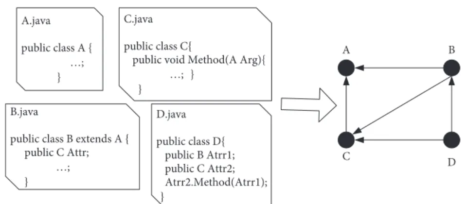
Files are key software components in the software sys-tem, and they are gathered up by interactions. SN at file level can be defined as in Figure 4: Every file is viewed as a single node in SN, and the dependency and association relation-ships between files are represented by edges (directed or undirected). Let SN� (V, E) represents the software net-work, where each file can be treated as noden_i(n_i∈V). The relationships between every pair of files, if exist, form a directed edgee_i(e_i∈E).

3.4. Network Embedding. Network embedding (EM) is to map information networks into low-dimensional spaces, in which every vertex is represented as a low-dimensional vector. Such a low-dimensional embedding is very useful in a variety of applications such as node classification [3], link prediction [10], and personalized recommendation [23]. So far, various network embedding methods have been pro-posed successively in the field of machine learning. In this paper, we adopt Node2vec algorithm to embedding learning of the token vector.

Node2vec performs a random walk on neighbor nodes and then sends the generated random walk sequences to the Skip-gram model for training. In Node2vec, a 2nd-order random walk with two parameters p and q are used to flexibly sample neighborhood nodes between BFS (breadth-first search) and DFS (depth-(breadth-first search).

Formally, given a source nodeu, we simulate a random walk of fixed lengthl. Letc_idenote theith node in the walk, starting withc₀�u. Nodec_i is generated by the following distribution: P c􏼐_i�x􏼌􏼌􏼌􏼌c_i−1�v􏼑� πvx Z, if(v, x)εE, 0, otherwise, ⎧ ⎪ ⎪ ⎪ ⎨ ⎪ ⎪ ⎪ ⎩ (2)

where πvx is the unnormalized transition probability be-tween nodevandx, andZis the normalized constant.

As shown in Figure 5, the unnormalized transition probability πvxsets to πvx�αpq(t, x) ·wvx, wheredtx rep-resents the shortest distance between node tandx:

αpq(t, x) � 1 p, ifdtx�0, 1, ifd_tx�1, 1 q, ifdtx�2. ⎧ ⎪ ⎪ ⎪ ⎪ ⎪ ⎪ ⎪ ⎪ ⎪ ⎪ ⎨ ⎪ ⎪ ⎪ ⎪ ⎪ ⎪ ⎪ ⎪ ⎪ ⎪ ⎩ (3)

4. Approach

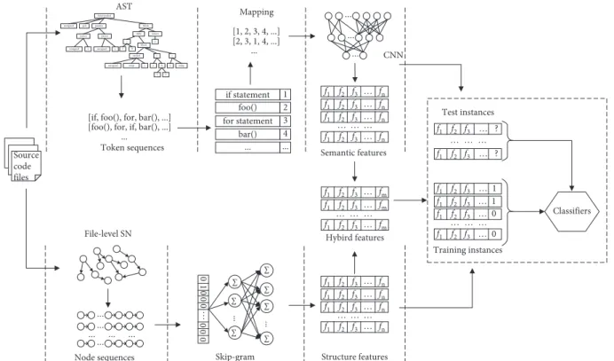
In this section, we elaborate our proposed method of software defect prediction via semantic and structural fea-tures from source code files (SDP-S2S). The overall framework of SDP-S2S is presented in Figure 6. It mainly

consists of three parts: the first part is the generation of semantic features from source codes and will be detailed in Section 4.1. The second part will be explained in Section 4.2, which focuses on the extraction of structural features from software network by network embedding learning. The last part refers to combining the semantic and structural features obtained in the first two steps into new features and used for software defect prediction.

4.1. Generation of Semantic Features. In order to achieve semantic features for each source code file, we should first map the source code files into ASTs and parse them as real-valued token vectors. After that, the token vectors are encoded and preprocessed, and then, the resulting token vectors are fed to CNN for feature learning to generate the semantic features. The generation process is described in detail in the following three steps.

4.1.1. Parsing AST. In order to represent the semantic features of source code files, we need to find the appropriate granularity as the representation of the source code. As previous study [8] has shown, AST can represent the se-mantic and structural information of source code with the most appropriate granularity. We first parse the source code files into ASTs by calling an open-source python package javalang. As treated in [9], we only select three types of nodes on ASTs as tokens: (1) nodes of method invocations and class instance creations, which are recorded as their corre-sponding names; (2) declaration nodes, i.e., method/type/ enum declarations, whose values are extracted as tokens; and (3) control flow nodes, such as while, if, and throw, are recorded as their node types. Three types of selected nodes are listed in Table 1.

We call javalang’s API to parse the source code into an AST. Given a path of the software source code, the token sequences of all files in the software will be output. As described in Algorithm 1, first traverse the source code files under path P, and each file is parsed into an AST via the PARSE-AST function. For each AST, we employ the pre-order traversal strategy to retrieve the three types of nodes selected in Table 1 and receive the final token sequence. 4.1.2. Token Sequence Preprocessing. Since CNN only ac-cepts inputs as numerical vectors, the token sequences generated from ASTs cannot be directly fed to CNN. Therefore, to get the numerical token vectors, it is necessary for the extracted token sequences to be converted into in-teger vectors. To do this, we give each token a unique inin-teger ID, and the ID of the recurring token is identical. Note that, because the token sequences of all files are of unequal length, the converted integer token vectors may differ in their di-mensions. Also, CNN requires input vectors to have the same length; hence, we append 0 to each integer vectors, making their lengths consistent with the longest vector. Additionally, during the encoding process, we filter out infrequent tokens which might be designed for a specific file and not generalized for other files. Specifically, we only

encode tokens occurring three or more times, while denote the others as 0.

In addition, for software defect prediction, the class imbalance of defect dataset often exists. Specifically, the number of clean instances vastly outnumbers that of de-fective instances. Assuming that the number of clean in-stances is labeled ass_nand the number of defective samples is sy, the imbalance rate (IR) [53] is used to measure the degree of imbalance:

IR�⌊sn

s_y⌋. (4)

The larger the IR, the greater the imbalance, and vice versa. Imbalance data will degrade the performance of our model. To address this issue, we duplicate the defective files several times until the IR index is close to 1.

4.1.3. Building CNN. In this paper, we adopt classic ar-chitecture of CNN for feature learning. After encoding and preprocessing token vectors, exclude the input and output layers; we train the CNN model with four layers, including an embedding layer (turn integer token vectors into real-valued vectors of fixed size), a convolutional layer, a max-pooling layer, and a fully connected layer. The overall ar-chitecture is illustrated in Figure 7.

ReLu activation functions are used for training, and the implementation is based on Keras (http://keras.io). The output layers are activated by sigmoid function and used

only for the parameters of the neural network weight matrix, to optimize the learning features. In addition, in this paper, Adam optimizer based on the improved stochastic gradient descent (SGD) algorithm is employed. Adam optimizer dynamically adjusts the learning rate for each parameter by calculating the first- and second-order moment estimations of the gradient. Compared with other optimization algo-rithms, Adam can ensure that the learning rate is distributed in an explicit range after each iteration, so that the parameter changes smoothly.

Given a projectP, suppose it containsnsource code files, all of which have been converted to integer token vectors x∈Rl _{and of equal length l by the treatments described} previously. Through the embedding layer, each token will be mapped to ad-dimension real-value vector. In other words, each file becomes a real-value matrixX_l×d. As the input of convolutional layer, a filterL∈Rh×d_{is applied to a region} ofhtokens to produce a new feature. For example, a feature fi is generated from a region of tokensxi:i+h−1 by

f_i�tanh L·x_i:i+h−1+b􏼁. (5)

Here,bis a bias term and tanh is a nonlinear hyperbolic tangent function. Each possible region of tokens in the description 􏼈x_1:h, x_2:h+1,. . ., x_i:i+h−1,. . ., x_l−h+1:l􏼉applies fil-ter Lto produce a feature map:

F�􏼂f₁, f₂,. . ., f_l−h+1􏼃, (6)

where f_i∈Rl−h+1_{. Then, a 1-max-pooling operation is} carried out over the mapped features and the maximum valueF􏽢�max􏼈 􏼉f is taken as the feature corresponding to this particular filterL. Usually, multiple filters with different region sizes are used to get multiple features. Finally, a fully connected layer further generated the semantic features.

4.2. Generation of Structural Features. Before applying network embedding to represent structural features of source codes, it is necessary to build a software network model according to source files. As we did in the previous studies [11, 12], we use DependencyFinder API to parse the compiled source files (.zip or .jar extension) and extract their relationships using a tool developed by ourselves. With the directed software network, we further perform embedding

A B C _D A.java public class A { …; } B.java

public class B extends A { public C Attr;

…; }

C.java public class C{

public void Method(A Arg){ …; } D.java public class D{ public B Atrr1; public C Attr2; Atrr2.Method(Atrr1); } }

Figure4: A single source code segment and its corresponding software network model at file level.

x1 x2 x3 t α = 1 v α = 1/q α = 1/q α = 1/p

learning using the Node2vec method. For more details on Node2vec, please refer to the literature [37].

4.3. Feature Concatenation. So far, we have got the semantic and structural features of source code files, respectively. Here, we label semantic feature as F_semantic and structural feature as F_structural. In order to verify the effectiveness of code semantic and structural features on software defect prediction, in addition to analyzing the impact of each type of generation feature on defect prediction, we also explore the impact of their combination. We directly concatenate the semantic feature vectors with structural feature vectors via Merge operator in Keras, and the resulting feature vectors presented asF_hybrid.

5. Experiment Setup

5.1. Dataset. In our study, 6 Apache open-source projects based on Java are selected (https://github.com/apache) and a

total of 12 defect datasets available at the PROMISE repository (http://promise.site.uottawa.ca/SERepository/datasets-page. html) are picked for validation. Detailed information on the datasets is listed in Table 2, where #Avg. (files) and #Avg. (defect rate) are the average number of files and the average percentage of defective files, respectively. An instance in the defect dataset represents a class file and consists of two parts: independent variables including the learned features (e.g., the CNN-learned semantic features) and a dependent variable labeled as defective or not in this class file.

5.2. Evaluation Measures. The essence of defect prediction in this study is a binary classification problem. Note that a binary classifier can make two possible errors: false positives and false negatives. In addition, a correctly classified de-fective class file is a true positive and a correctly classified clean class file is a true negative. We evaluate the classifi-cation results in terms of Precision, Recall, and F-measure, which are described as follows:

Source code files AST functionded unsigned gcd params param param x y unsigned unsigned block return while > 0 x y block = varded = x y unsigned temp % y temp

x y

[if, foo(), for, bar(), ...] [foo(), for, if, bar(), ...]

... if statement 1 foo() 2 for statement 3 bar() 4 ... ... [1, 2, 3, 4, ...] [2, 3, 1, 4, ...] ... .. . .. . .. . f1 f2 f3 f1 f2 f3 … fn f1 f2 f3 … fn f1 f2 f3 … fn f1 f2 f3 … fn f1 f2 f3 … fm … … … f1 f2 f3 … fn f1 f2 f3 … fn f1 f2 f3 … fn f1 … … …f2 f3 … fn … 1 … … … … 1 … 0 … 0 … ? … ? … … … Classifiers Training instances Test instances .. . .. . .. . .. . ... ...

Node sequences Skip-gram

∑ ∑ ∑ ∑ ∑ ∑ ∑ ... ... 01 0 0 0 … 00 0 … … … Structure features Semantic features Hybird features Token sequences Mapping CNN File-level SN f1 f2 f3 … fm f1 f2 f3 … fm f1 f2 f3 f1 f2 f3 f1 f2 f3 f1 f2 f3 f1 f2 f3

Figure6: The overall framework of our approach.

Table1: The selected AST nodes.

ID Node types AST node record

Node₁ Method invocations and class

instance creations MethodInvocation, SuperMethodInvocation, MemberReference, SuperMemberReference Node2 Declaration nodes

PackageDeclaration, InterfaceDeclaration, ClassDeclaration, MethodDeclaration, ConstructorDeclaration, VariableDeclarator, CatchClauseParameter, FormalParameter ,

TryResource, ReferenceType, BasicType

Node3 Control flow nodes

IfStatement, WhileStatement, DoStatementForStatement, AssertStatement, BreakStatementContinueStatement, ReturnStatement, ThrowStatement, SynchronizedStatement, TryStatement, SwitchStatementBlockStatement,

Precision� true positive

true positive+false positive,

Recall� true positive

true positive+false negative,

F−measure�2∗Precision∗Recall

Precision+Recall .

(7)

False positive refers to the predicted defective files that actually have no defects, and false negative refers to the actually defect-prone files predicted as clean. Precision and Recall are mutually exclusive in practice. Therefore, F -measure, as a weighted average of Precision and Recall, is

more likely to be adopted. The value of F-measure ranges between 0 and 1, with values closer to 1 indicating better performance for classification results.

5.3. Experiment Design. First, to make a comparison be-tween the traditional hand-crafted features and automati-cally learn features in our context, four scenarios will be considered in our experiments.

(i) SDP-base represents software defect prediction based on the traditional hand-crafted features (ii) SDP-S1 represents software defect prediction based

on the semantic featuresF_semantic

Input: pathpof the software source code

Output: token sequences for all file

(1)functionEXTRACT (Pathp)

(2) F�the set of source code files under pathp; (3) foreachf∈Fdo

(4) create sequences_file−token; (5) s_file−token⟵PARSE−AST(f);

(6) returns_file−token;

(7) end for

(8)end function

(9)functionPARSE-AST (Filef)

(10) create sequences_token;

(11) root⟵javalang.parseFile2AST(f);

(12) for allASTNodek∈rootdo

(13) ifk∈Node1then

(14) record its name and append tos_token;

(15) else ifk∈Node2then

(16) record its declared value and append tos_token;

(17) else ifk∈Node3then

(18) record its type and append tos_token;

(19) end if

(20) end for

(21) returns_token

(22)end function

ALGORITHM 1: Parse-AST and return the token sequence of each file.

Preprocessing token vectors Real-value vector matrix Semantic features

Embedding layer Convolutional layer Pooling layer

Full connected layer

(iii) SDP-S2 represents software defect prediction based on the structural featuresF_structural

(iv) SDP-S2S represents software defect prediction based on the semantic and structural featuresF_hybrid Second, we will further explore prediction performance under different parameter settings for CNN and network embedding learning. For each project, note that we use the data from the older version to train the CNN model. Then, the trained CNN is used to generate semantic and structural features for both the older and newer versions. After that, we use the older version to build a defect prediction model and apply it to the newer version.

5.4. Experimental Results

5.4.1. Impact of Different Features. For each type of feature, Table 3 shows some interesting results: except for few cases (Poi), theF-measure values of S1, S2, and SDP-S2S are greater than those of the benchmark SPD-base, implying a significant improvement in accuracy. For ex-ample, for Camel, the growth rate of performance is more than 21.7%, when using the learned semantic and/or structural features. Especially when semantic and structural features are used comprehensively, the advantage is more obvious, indicated by the 99.5% performance growth. Ad-ditionally, note that for Xerces, although the growth rates of performance are slightly lower than that of Camel, it is still considerable, around 30%. For Lucene, Synapse, and Xalan, the corresponding maximum growth rates are 27.9% (0.7564), 22.6% (0.5204), and 10% (0.2406), respectively. The majority of positive growth rates suggest the feasibility of our proposed method of automatically learning features from source code files.

In Table 3, the results also show that SDP-S2S performs better than SDP-S1 and SDP-S2, indicated by more F -measure values in bold. Specifically, compared to the other two methods, SDP-S2S achieves the best performance on projects Camel, Lucene, and Xerces. In order to better distinguish their influences on defect prediction, we make further comparisons in terms of the Wilcoxon signed-rank test (p-value) and Cliff’s effect size from a statistical per-spective. In Table 4, the Wilcoxon signed-rank test highlights that there is no significant performance difference among the three predictors, indicated by the Sig. p>0.01. However, when it comes to the Cliff’s effect size delta, the negative values show that their effect size is different. Specifically, SDP-S2 outperforms SDP-S1, whereas SDP-S2S outper-forms SDP-S2.

With the evidences provided by the above activities, the approach of feature learning proposed in this paper is validated to be suitable for defect prediction.

5.4.2. Parameter Sensitivity Analysis

(1) Parameter Analysis of CNN. When using CNN to rep-resent semantic features, the setting of some parameters of the network layer will affect the representation of semantic features and thus affect prediction performance. In this section, according to the key parameters of CNN, including the length of filter, the number of filters, and embedding dimensions, we tune the three parameters by conducting experiments with different values of the parameters. Note that, for other parameters, we directly present their values obtained from previous studies [9]: batch size is set as 32 and the training epoch is 15. By fixing other parameters, we analyze the influence of the three parameters on the results, respectively.

Figures 8–10, respectively, present the performance obtained under different filter lengths, different number of filters, and different embedding dimensions. It is not hard to

Table2: Details of the datasets.

Project Releases Avg. (#files) Avg. (defect rate) (%) IR (imbalance rate)

Camel 1.4, 1.6 892 18.6 5.01 Lucene 2.0, 2.2 210 55.7 1.14 Poi 2.5, 3.0 409 64.7 0.55 Synapse 1.1, 1.2 239 30.5 2.70 Xalan 2.5, 2.6 815 48.5 1.07 Xerces 1.2, 1.3 441 15.5 5.20

Table3:F-measure values of defect prediction built with four types

of features. Projects SDP-base SDP-S1 (△%) SDP-S2 (△%) SDP-S2S (△%) Camel 0.2531 0.5044 (99.3%) 0.3081 (21.7%) 0.5049 (99.5%) Lucene 0.5912 0.6397 (8.2%) 0.6873 (16.3%) 0.7564 (27.9%) Poi 0.7525 ₍0.7250 −3.7%) 0.7892 (4.9%) 0.7340 (−2.5%) Synapse 0.4244 0.4444 (4.7%) 0.5204 (22.6%) 0.4390 (3.4%) Xalan 0.6165 0.6780 (10.0%) 0.6229 (1.0%) 0.6623 (7.4%) Xerces 0.1856 0.2406 (29.6%) 0.2432 (31.0%) 0.2650 (42.8%)

△% represents the growth rate of performance relative to SDP-base.

Table4: Comparison of the distributions of three methods in terms

of the Wilcoxon signed-rank test and Cliff’s effect size.

Sig. p<0.01 Cliff’s delta

SDP-S1 vs. SDP-S2 0.753 −0.056

SDP-S1 vs. SDP-S2S 0.345 −0.167

find that all six curves reach the highest performance when the filter length is set to 10. The optimal number of filters is 20, where the performance generally reaches the peak. In-terestingly, for project Xerces, when the number of filters is set as 100, the performance becomes particularly bad. With regard to the embedding dimensions, six curves on the whole are very stable, which means that the dimension of representation vector has a very limited impact on the prediction performance.

(2) Parameter Analysis of Software Network Embedding. For the generation of structural features, in Node2vec, a pair of parametersp andqcontrolling random walk will affect the learning. That is, different combinations ofpand q determine the different ways of random walk in the process of network embedding and then generate different structural features. Therefore, we further analyze the two parameters.

Take Poi and Synapse, for example, we construct 25 groups of (p, q) and let p, q∈[0.25,0.5,1,2,4]. With different combinations (p,q), the results are as shown in Figure 11 and the effect of different combinations is different. For example, when the combination (p,q) is set as (4, 2) in Poi, the best performance 0.789 is achieved, and yet the suitable combinations (p, q) is (0.5, 0.25) in Synapse, and theF-measure value is 0.5204. Therefore, for each project in our context, we give out the optimal combination (p, q), shown in Table 5, so as to learn the defect structural information and generate corresponding structural features better.

6. Threats to Validity

To evaluate the feasibility of our method in defect pre-diction, we constructed four kinds of predictors according to different features and compared their per-formance. In this paper, although we do not explicitly compare with the state-of-the-art defect prediction techniques, SDP-S1 is actually equivalent to the method proposed in the literature [13]. Since the original implementation of CNN is not released, we have reproduced a new version of CNN via Keras. Throughout, we strictly followed the procedures and parameters set-tings described in the reference, such as the selection of AST nodes and the learning rate when training neural networks. Therefore, we are confident that our imple-mentation is very close to the original model.

In this paper, our experiments were conducted with defect datasets of six open-source projects from the PROMISE repository, which might not be representative of all software projects. More projects that are not included in this paper or written in other programming languages are still to be considered. Besides, we only evaluated our ap-proach in terms of different features and did not compare with other state-of-the-art prediction methods. To make our approach more generalizable, in the future, we will conduct experiments on a variety of projects and compare with more benchmark methods. Camel Synapse Lucene Xalan Poi Xerces 0.2 0.3 0.4 0.5 0.6 0.7 0.8 0.9 F -me asure 3 5 10 20 50 100 2 Filter length

Figure8: Different filter lengths.

Camel Synapse Lucene Xalan Poi Xerces 0.2 0.3 0.4 0.5 0.6 0.7 0.8 0.9 F -measure 10 20 50 100 150 200 5 Number of filters

Figure9: Different number of filters.

Camel Synapse Lucene Xalan Poi Xerces 0.2 0.3 0.4 0.5 0.6 0.7 0.8 F -measure 20 30 40 50 60 70 10 Dimensions

7. Conclusion

This study aims to build better predictors by learning as much defect feature information as possible from source code files, to improve the performance of software defect predictions. In summary, this study has been conducted on 6 open-source projects and consists of (1) an empirical vali-dation on the feasibility of the structural features that learned from software network at the file level, (2) an in-depth analysis of our method SDP-S2S combined with se-mantic features and structural features, and (3) a sensitivity analysis with regard to the parameters in CNN and network embedding.

Compared with the traditional hand-crafted features, the F-measure values are generally increased, the maximum is up to 99.5%, and the results indicate that the inclusion of structural features does improve the performance of SDP. Statistically, the advantages of SDP-S2S are particularly obvious from the perspective of Cliff’s effect size. More specifically, the combination of semantic features and structural features is the preferred selection for SDP. In addition, our results also show that the filter length is preferably 10, the optimal number of filters is 20, and the dimension of the representation vector has a very limited impact on the prediction performance. Finally, we also analyzed the parameterspandqinvolved in the embedding learning process of software network.

Our future work mainly includes two aspects. On the one hand, we plan to validate the generalizability of our study with more projects written in different languages. On the other hand, we will focus on more effective strategies such as feature selection techniques. Last but not least, we also plan

to discuss the possibility of considering not only CNN and Node2vec model but also RNN or LSTM for learning se-mantic features and graph neural networks for network embedding, respectively.

Data Availability

The experimental data used to support the findings of this study are available at https://pan.baidu.com/s/ 1H6Gw7UHb7vfBFFVfDBF6mQ.

Conflicts of Interest

The authors declare that they have no conflicts of interest.

Acknowledgments

This work was supported by the National Key Research and Development Program of China (2018YFB1003801); the National Natural Science Foundation of China (61902114); Hubei Province Education Department Youth Talent Project (Q20171008); and Hubei Provincial Key Laboratory of Applied Mathematics (HBAM201901).

References

[1] P. He, B. Li, X. Liu, J. Chen, and Y. Ma, “An empirical study on software defect prediction with a simplified metric set,” In-formation and Software Technology, vol. 59, pp. 170–190, 2015. [2] E. N. Adams, “Minimizing cost impact of software defects,” Report RC, IBM Research Division, New York, NY, USA, 1980.

[3] P. Yu, F. Yang, C. Cao et al., “API usage change rules mining based on fine-grained call dependency analysis,” in Pro-ceedings of the 2017 Asia-Pacific Symposium on Internetware, ACM, Shanghai, China, 2017.

[4] T. T. Nguyen, H. A. Nguyen, N. H. Pham et al., “Graph-based mining of multiple object usage patterns,” inProceedings of the 2009 ACM SIGSOFT International Symposium on Foundations of Software Engineering, pp. 24–28, Amsterdam, Nethelands, 2009.

[5] B. Cui, J. Li, T. Guo et al., “Code comparison system based on Abstract syntax tree,” in Proceedings of the 2010 IEEE 0.4 0.5 0.6 0.7 0.8 0.9 F -measure 3 5 7 9 11 13 15 17 19 21 23 25 1 The id of (p, q) combinations (a) 0 0.1 0.2 0.3 0.4 0.5 0.6 F -measure 3 5 7 9 11 13 15 17 19 21 23 25 1 The id of (_p, _q) combinations (b)

Figure11: Results of different combinations ofpandq. (a) Poi. (b) Synapse.

Table5: The combination ofpandqselected in this paper.

Project p q Camel 2 1 Lucene 0.25 4 Poi 4 2 Synapse 0.5 0.25 Xalan 4 1 Xerces 0.5 4

International Conference on Broadband Network & Multimedia Technology, pp. 668–673, IEEE, Beijing, China, October 2010. [6] S. Q. de Medeiros, G. D. A. Alvez Junior, and F. Mascarenhas, “Automatic syntax error reporting and recovery in parsing expression grammars,” 2019, https://arxiv.org/abs/1905. 02145.

[7] F. Deqiang, X. Yanyan, Y. Haoran, and B. Yang, “WASTK: a weighted Abstract syntax tree kernel method for source code plagiarism detection,” Scientific Programming, vol. 2017, Article ID 7809047, 8 pages, 2017.

[8] S. Wang, T. Liu, and L. Tan, “Automatically learning semantic features for defect prediction,” inProceedings of the 38th IEEE International Conference on Software Engineering, pp. 297– 308, IEEE, Austin, TX, USA, May 2016.

[9] J. Li, P. He, J. Zhu, and M. R. Lyu, “Software defect prediction via convolutional neural network,” inProceedings of the 2017 IEEE International Conference on Software Quality, Reliability and Security (QRS), pp. 318–328, IEEE, Prague, Czech Re-public, July 2017.

[10] W. Pan, B. Li, Y. Ma, and Y. J. Liu, “Multi-granularity evo-lution analysis of software using complex network theory,” Journal of Systems Science and Complexity, vol. 24, no. 6, pp. 1068–1082, 2011.

[11] H. E. Peng, P. Wang, L. I. Bing et al., “An evolution analysis of software system based on multi-granularity software net-work,”Acta Electronica Sinica, vol. 46, no. 2, pp. 257–267, 2018.

[12] P. He, B. Li, Y. Ma, and L. He, “Using software dependency to bug prediction,” Mathematical Problems in Engineering, vol. 2013, Article ID 869356, 12 pages, 2013.

[13] D. Zhang, J. Yin, X. Zhu, and C. Zhang, “Network repre-sentation learning: a survey,”IEEE Transactions on Big Data, vol. 6, no. 1, pp. 3–28, 2018.

[14] D. Radjenovi´c, M. Heriˇcko, R. Torkar, and A. ˇZivkoviˇc, “Software fault prediction metrics: a systematic literature review,”Information & Software Technology, vol. 55, no. 8, pp. 1397–1418, 2013.

[15] T. J. McCabe, “A complexity measure,”IEEE Transactions on Software Engineering, vol. SE-2, no. 4, pp. 308–320, 1976. [16] S. R. Chidamber and C. F. Kemerer, “A metrics suite for object

oriented design,”IEEE Transactions on Software Engineering, vol. 20, no. 6, pp. 476–493, 1994.

[17] J. Bansiya and C. G. Davis, “A hierarchical model for object-oriented design quality assessment,” IEEE Transactions on Software Engineering, vol. 28, no. 1, pp. 4–17, 2002. [18] R. Moser, W. Pedrycz, and G. Succi, “A comparative analysis

of the efficiency of change metrics and static code attributes for defect prediction,” inProceedings of the 2008 ACM/IEEE International Conference on Software Engineering, pp. 181– 190, IEEE, Leipzig, Germany, May 2008.

[19] N. Nagappan and T. Ball, “Using software dependencies and churn metrics to predict field failures: an empirical case study,” inProceedings of the 2007 International Symposium on Empirical Software Engineering & Measurement, pp. 364–373, IEEE, Madrid, Spain, September 2007.

[20] A. E. Hassan, “Predicting faults using the complexity of code changes,” inProceedings of the 31st International Conference on Software Engineering, pp. 78–88, IEEE, Vancouver, Can-ada, May 2009.

[21] J. Nam, W. Fu, S. Kim, T. Menzies, and L. Tan, “Heteroge-neous defect prediction,” IEEE Transactions on Software Engineering, vol. 44, no. 9, pp. 874–896, 2018.

[22] T. Wolf, A. Schroter, D. Damian, and T. Nguyen, “Predicting build failures using social network analysis on developer

communication,” inProceedings of the 2009 IEEE 31st In-ternational Conference on Software Engineering, pp. 1–11, Vancouver, Canada, May 2009.

[23] M. Soto, Z. Coker, and C. L. Goues, “Analyzing the impact of social attributes on commit integration success,” in Pro-ceedings of the 2017 IEEE/ACM 14th International Conference on Mining Software Repositories, ACM, 2017, DOI: 10.1109/ MSR.2017.34.

[24] R. Kumar and K. P. Singh, “SVM with feature selection and extraction techniques for defect-prone software module prediction,” inProceedings of 6th International Conference on Soft Computing for Problem Solving, pp. 279–289, Springer, Singapore, 2017.

[25] N. Fenton, M. Neil, W. Marsh, P. Hearty, Ł. Radli´nski, and P. Krause, “On the effectiveness of early life cycle defect prediction with Bayesian nets,” Empirical Software Engi-neering, vol. 13, no. 5, pp. 499–537, 2008.

[26] ¨O. F. Arar and K. Ayan, “A feature dependent naive Bayes approach and its application to the software defect prediction problem,”Applied Soft Computing, vol. 59, pp. 197–209, 2017. [27] Q. Cao, Q. Sun, Q. Cao, and H. Tan, “Software defect pre-diction via transfer learning based neural network,” in Pro-ceedings of the 2015 1st International Conference on Reliability Systems Engineering, pp. 1–10, Beijing, China, October 2015. [28] Z. Li, X.-Y. Jing, X. Zhu, H. Zhang, B. Xu, and S. Ying, “Heterogeneous defect prediction with two-stage ensemble learning,” Automated Software Engineering, vol. 26, no. 3, pp. 599–651, 2019.

[29] B. Turhan, T. Menzies, A. B. Bener, and J. Di Stefano, “On the relative value of cross-company and within-company data for defect prediction,”Empirical Software Engineering, vol. 14, no. 5, pp. 540–578, 2009.

[30] J. Nam, S. Pan, and S. Kim, “Transfer defect learning,” in Proceedings of the 35th International Conference on Software Engineering (ICSE), pp. 382–391, IEEE, San Francisco, CA, USA, May 2013.

[31] X. Yang, D. Lo, X. Xia, Y. Zhang, and J. Sun, “Deep learning for just-in-time defect prediction,” inProceedings of the 2015 IEEE International Conference on Software Quality, Reliability and Security (QRS), IEEE, 2015.

[32] A. V. Phan, M. L. Nguyen, and L. T. Bui, “Convolutional neural networks over control flow graphs for software defect prediction,” 2018, https://arxiv.org/abs/1802.04986.

[33] T. Zimmermann and N. Nagappan, “Predicting defects using network analysis on dependency graphs,” inProceedings of the 30th International Conference on Software Engineering, pp. 531–540, IEEE, Leipzig, Germany, May 2008.

[34] H. Abandah and I. Alsmadi, “Dependency graph and metrics for defects prediction,”International Journal of ACM Jordan, vol. 2, no. 3, pp. 115–119, 2013.

[35] P. Bhattacharya, M. Iliofotou, I. Neamtiu, and M. Faloutsos, “Graph-based analysis and prediction for software evolution,” in Proceedings of the International Conference on Software Engineering, pp. 419–429, IEEE, Zurich, Switzerland, June 2012.

[36] B. Perozzi, R. Al-Rfou, and S. Skiena, “DeepWalk: online learning of social representations,” 2014, https://arxiv.org/ abs/1403.6652.

[37] A. Grover and J. Leskovec, “node2vec: scalable feature learning for networks,” in Proceedings of the 2016 ACM SIGKDD International Conference on Knowledge Discovery & Data Mining, San Francisco, CA, USA, August 2016. [38] J. Tang, M. Qu, M. Wang, M. Zhang, J. Yan, and Q. Mei,

Proceedings of the 24th International Conference on World Wide Web, pp. 1067–1077, Florence, Italy, May 2015. [39] G. Concas, C. Monni, M. Orru et al., “Software systems

through complex networks science: review, analysis and ap-plications,” inProceedings of the 4th International Workshop on Emerging Trends in Software Metrics, pp. 14–20, San Francisco, CA, USA, May 2012.

[40] A. Gu, X. Zhou, Z. Li, Q. Li, and L. Li, “Measuring object-oriented class cohesion based on complex networks,”Arabian Journal for Science and Engineering, vol. 42, no. 8, pp. 3551– 3561, 2017.

[41] H. H. Zhang, W. J. Feng, and L. J. Wu, “The static structural complexity metrics for large-scale software system,”Applied Mechanics and Materials, vol. 44–47, pp. 3548–3552, 2010. [42] Y.-T. Ma, K.-Q. He, B. Li, J. Liu, and X.-Y. Zhou, “A hybrid set

of complexity metrics for large-scale object-oriented software systems,”Journal of Computer Science and Technology, vol. 25, no. 6, pp. 1184–1201, 2010.

[43] W. Pan and C. Chai, “Measuring software stability based on complex networks in software,”Cluster Computing, vol. 22, no. S2, pp. 2589–2598, 2019.

[44] Q. Gu and D. Chen, “Validation and simulation of software system evolution rules using software networks,” Science China, vol. 44, no. 1, pp. 20–36, 2014.

[45] S. M. Srinivasan, R. S. Sangwan, and C. J. Neill, “On the measures for ranking software components,”Innovations in Systems and Software Engineering, vol. 13, no. 2-3, pp. 161– 175, 2017.

[46] W. Pan, H. Ming, C. K. Chang, Z. Yang, and D.-K. Kim, “ElementRank: ranking Java software classes and packages using multilayer complex network-based approach,” IEEE Transactions on Software Engineering, p. 1, 2019.

[47] W. Pan, B. Li, J. Liu, Y. Ma, and B. Hu, “Analyzing the structure of Java software systems by weighted k-core de-composition,”Future Generation Computer Systems, vol. 83, pp. 431–444, 2018.

[48] W. Pan, B. Song, K. Li, and K. Zhang, “Identifying key classes in object-oriented software using generalized k-core de-composition,”Future Generation Computer Systems, vol. 81, pp. 188–202, 2018.

[49] I. Goodfellow, Y. Bengio, and A. Courville,Deep Learning, MIT Press, Cambridge, MA, USA, 2016, http://www. deeplearningbook.org.

[50] T. N. Sainath, B. Kingsbury, A. R. Mohamed et al., “Im-provements to deep convolutional neural networks for LVCSR,” inProceedings of the 2013 IEEE Workshop on Au-tomatic Speech Recognition and Understanding, pp. 315–320, Olomouc, Czech Republic, December 2013.

[51] A. Krizhevsky, I. Sutskever, and G. Hinton, “ImageNet classification with deep convolutional neural networks,” Advances in Neural Information Processing Systems, Springer, vol. 25, no. 2, , pp. 1–9, Berlin, Germany, 2012.

[52] D. Maturana and S. Scherer, “VoxNet: a 3D convolutional neural network for real-time object recognition,” in Pro-ceedings of the 2015 IEEE/RSJ International Conference on Intelligent Robots and Systems (IROS), pp. 922–928, IEEE, Hamburg, Germany, September 2015.

[53] M. Galar, A. Fernandez, E. Barrenechea, H. Bustince, and F. Herrera, “A review on ensembles for the class imbalance problem: bagging-, boosting-, and hybrid-based approaches,” IEEE Transactions on Systems, Man, and Cybernetics, Part C (Applications and Reviews), vol. 42, no. 4, pp. 463–484, 2012.