The distribution of neutral hydrogen around high-redshift galaxies
and quasars in the EAGLE simulation
Alireza Rahmati,
1,2‹Joop Schaye,
3Richard G. Bower,
4Robert A. Crain,
5,3Michelle Furlong,
4Matthieu Schaller
4and Tom Theuns
41Institute for Computational Science, University of Z¨urich, Winterthurerstrasse 190, CH-8057 Z¨urich, Switzerland 2Max-Planck Institute for Astrophysics, Karl-Schwarzschild-Strasse 1, D-85748 Garching, Germany
3Leiden Observatory, Leiden University, PO Box 9513, NL-2300 RA Leiden, the Netherlands
4Institute for Computational Cosmology, Department of Physics, University of Durham, South Road, Durham DH1 3LE, UK 5Astrophysics Research Institute, Liverpool John Moores University, 146 Brownlow Hill, Liverpool L3 5RF, UK
Accepted 2015 June 23. Received 2015 May 6; in original form 2015 March 18
A B S T R A C T
The observed high covering fractions of neutral hydrogen (HI) with column densities
above ∼1017cm−2 around Lyman-Break Galaxies (LBGs) and bright quasars at redshifts
z∼2–3 has been identified as a challenge for simulations of galaxy formation. We use the Evolution and Assembly of Galaxies and their Environment (EAGLE) cosmological, hydrody-namical simulation, which has been shown to reproduce a wide range of galaxy properties and for which the subgrid feedback was calibrated without considering gas properties, to study the distribution of HIaround high-redshift galaxies. We predict the covering fractions of strong HI
absorbers (NHI 1017cm−2) inside haloes to increase rapidly with redshift but to depend only weakly on halo mass. For massive (M2001012M) haloes, the covering fraction profiles are
nearly scale-invariant and we provide fitting functions that reproduce the simulation results. While efficient feedback is required to increase the HIcovering fractions to the high observed
values, the distribution of strong absorbers in and around haloes of a fixed mass is insensitive to factor of 2 variations in the strength of the stellar feedback. In contrast, at fixed stellar mass the predicted HIdistribution is highly sensitive to the feedback efficiency. The fiducial
EAGLE simulation reproduces both the observed global column density distribution function of HIand the observed radial covering fraction profiles of strong HIabsorbers around LBGs
and bright quasars.
Key words: methods: numerical – galaxies: formation – galaxies: high-redshift – intergalactic medium – quasars: absorption lines.
1 I N T R O D U C T I O N
Galaxies need to acquire large quantities of fresh gas from the in-tergalactic medium (IGM) to sustain their star formation activities through time (e.g. Bauermeister, Blitz & Ma 2010). Simulations predict that a large fraction of the accreting material enters haloes relatively cold and could therefore contain significant amounts of neutral gas (e.g. Fumagalli et al.2011; van de Voort et al.2012). The presence of shock-heated gas complicates the journey of the accreting gas on to galaxies. Moreover, energetic feedback from stars and active galactic nuclei (AGN), which regulate the con-sumption of the accreted gas and launch galactic outflows, affect the dynamics and chemical composition of gas around galaxies. As
E-mail:[email protected]
a result, the complex distribution of gas around galaxies contains the finger-prints of the aforementioned processes and studying it, mostly by analysing the absorption signature of neutral hydrogen and metals in the spectra of bright background sources, is of great value for understanding galaxies and the physical processes that regulate them.
Observations and simulations show that both the number of HI
absorbers and their typical column densities increase closer to galax-ies (e.g. Adelberger et al.2003; Chen & Mulchaey2009; Rakic et al.
2012; Rahmati & Schaye2014; Turner et al.2014). This suggests that absorbers with higher HIcolumn densities are better probes
of the gas in the vicinity of galaxies. Cosmological simulations, however, suggest that most strong HI absorbers, such as
Ly-man Limit Systems (LLSs; withNHI10
17.2cm−2) and Damped
Lyman αsystems (DLAs; withNHI10
20.5cm−2), are close to
galaxies that are too faint to be easily detectable in current surveys
(Rahmati & Schaye2014), which is in agreement with the lack of detected counterparts close to most of strong HIabsorbers (e.g.
Fu-magalli et al.2015). Not knowing the properties of the host galaxy complicates the use of strong HIabsorbers to study the relation
between galaxies and their environments. This problem can, how-ever, be circumvented by studying the distribution of HIabsorbers
around easily detectable bright galaxies.
Several modern observational campaigns have adopted this galaxy-centred approach by using quasar absorption lines to sys-tematically investigate the distribution of neutral hydrogen around massive galaxies at different epochs (e.g. Adelberger et al.2003; Hennawi et al.2006; Chen & Mulchaey2009; Rakic et al.2012; Prochaska, Hennawi & Simcoe 2013a; Tumlinson et al. 2013; Turner et al.2014). For instance, Rudie et al. (2012) measured the covering fraction of HIaround Lyman-Break galaxies (LBGs) atz∼2 and found that there is an∼30 per cent chance for finding LLSs in the spectra of background quasars that have impact param-eters less than∼100 proper kpc (hereafter pkpc). Noting that this impact parameter is comparable to the virial radii of LBGs atz∼2, this result implies that LLSs have a covering fraction of 30 per cent within the virial radius of LBGs. Prochaska et al. (2013b) showed that the abundance of HIabsorbers is significantly enhanced out
to several virial radii from bright quasars atz ∼ 2. They found that there is a more than 60 per cent chance of finding an LLS within∼150 pkpc from a bright quasar (Prochaska et al.2013a), which is comparable to the typical virial radius of the haloes with
M200∼1012.5M
that are expected to host the observed quasars at
z∼2.
Motivated by recent observational constraints, several groups used simulations to study the distribution of HI around galaxies
(e.g. Faucher-Gigu`ere & Kereˇs2011; Fumagalli et al.2011,2014; Rakic et al.2013; Shen et al.2013; Erkal2015; Meiksin, Bolton & Tittley2014; Faucher-Gigu`ere et al.2015). However, reproducing the relatively large observed covering fractions of strong HI
absorp-tion around massive galaxies turned out to be a major challenge (e.g. Fumagalli et al.2014; Faucher-Gigu`ere et al.2015).
Previous studies of high column density HI around massive
galaxies were based on the analysis of simulations that zoom into only one galaxy (e.g. Faucher-Gigu`ere & Kereˇs2011; Shen et al.
2013), or a handful of galaxies spanning a limited range in mass and redshift (e.g. Fumagalli et al.2011, 2014; Faucher-Gigu`ere et al. 2015). Given the diversity of observed galaxies, one may expect a large intrinsic variation in the spatial distribution of HI
from one galaxy to another. Consequently, a large sample of sim-ulated galaxies is required to predict the average distribution of HI and to compare it robustly with observations. Because
ob-servational constraints are at present limited to galaxies residing in relatively massive haloes (M200 1012M
), which are rare, especially at high redshifts, simulating a large number of them requires large cosmological volumes. Moreover, without cosmo-logical simulations it is not straightforward to check whether the simulations satisfy other important constraints on the cosmic dis-tribution of HI, for instance the global HI column density
dis-tribution function (CDDF) and/or the HI cosmic density, which
has been reproduced successfully in recent cosmological simula-tions (e.g. Altay et al. 2011; McQuinn, Oh & Faucher-Gigu`ere
2011; Dav´e et al.2013; Rahmati et al.2013a; Vogelsberger et al.
2014). The aforementioned issues may limit the power of stud-ies that use small numbers of zoom simulations and indicate that cosmological simulations of representative volumes are needed to study the average distribution of HIaround large numbers of
galaxies.
The strength and implementation of feedback mechanisms are also crucial factors for simulations of the distribution of gas around galaxies (e.g. Faucher-Gigu`ere et al. 2015; Suresh et al.2015). For instance, galactic winds driven by stellar feedback can change the distribution of HIaround galaxies by carrying the cold neutral
gas farther away from galaxies and by providing resistance against the accretion of gas. While feedback implementations vary widely, simulations that use strong stellar feedback have been more suc-cessful in reproducing the LLS covering fractions observed around LBGs (e.g. Shen et al.2013; Faucher-Gigu`ere et al.2015), which are significantly underproduced in simulations with weak feedback (e.g. Faucher-Gigu`ere & Kereˇs2011; Fumagalli et al.2011,2014). Moreover, feedback from AGN, which is required to form rea-sonable galaxies in very massive haloes and is missing from most previous studies, may affect the observed HI distribution in and around haloes expected to host quasars atz ∼2. However, sev-eral simulations indicate that only the strongest absorbers, which on average reside closer to or even inside galaxies, are significantly affected by feedback (e.g. Theuns et al.2002; Altay et al.2013; Bird et al.2014; Rahmati & Schaye2014). Hence, the more important effect may be that feedback changes the relation between stellar mass and halo mass and thus the predicted HIdistribution at fixed
stellar mass (e.g. Rakic et al.2013).
In this work, we study the HIdistribution around galaxies us-ing state-of-the-art cosmological hydrodynamical simulations. For this purpose, we use the Evolution and Assembly of Galaxies and their Environment (EAGLE) simulations (Schaye et al.2015, here-afterS15). The large cosmological volume of the main EAGLE run (100 cMpc) together with its relatively high resolution for a simu-lation of this type, allow us to study large numbers of haloes with masses similar to those targeted by recent observations, without compromising the resolution needed to simulate the distribution of relevant HIsystems (e.g. LLSs). Efficient stellar and AGN feedback enables the simulation to successfully reproduce a large number of basic observed characteristics of galaxies over wide mass and red-shift ranges (S15; Furlong et al.2015; Schaller et al.2015; Crain et al.2015) andS15already showed that EAGLE also reproduces the observed present-day column density distributions of CIVand
OVI. These factors make EAGLE ideal for studying the gas
distri-bution around galaxies.
We combine the EAGLE simulations with the accurate photoion-ization corrections from Rahmati et al. (2013a), which are based on high-resolution radiative transfer calculations. After showing the success of the simulation in reproducing the observed cosmic distribution of HI, we look at the HIdistribution around galaxies
fromz=4 to 1, bracketing the era during which the cosmic star formation density peaked. We focus on the strong HIabsorbers whose high covering fractions were found to be difficult to repro-duce by previous simulations (e.g. Faucher-Gigu`ere & Kereˇs2011; Fumagalli et al.2011,2014; Faucher-Gigu`ere et al.2015). We pre-dict that strong HIabsorbers, such as LLSs and DLAs, have a mean
covering fraction within the virial radius that increases rapidly with redshift, but depends only weakly on the halo mass (or star for-mation rate) at fixed redshift, suggesting that the distribution of absorbing gas around galaxies has a similar shape for different halo masses. Indeed, we show that the covering fraction of LLSs, sub DLAs and DLAs around massive galaxies (M2001012M
) fol-lows profiles with similar shapes but different scalelengths that are tied to the virial radius and redshift.
quasars, respectively. Accounting for the uncertainties in the ampli-tude of the ultra violet background (UVB) photoionization rate, our predictions are in excellent agreement with the observed HI
distri-butions. This shows that cosmological hydrodynamical simulations that are successful in reproducing reasonable galaxy properties, are also capable of predicting gas distributions in agreement with cur-rent observations. We conclude that there is no obvious missing ingredient in our general understanding of galaxy formation and evolution required to explain the observed HIdistributions around
LBGs and bright quasars atz∼2.
The structure of this paper is as follows. In Section 2, we intro-duce our cosmological simulations and discuss the photoionization corrections required for obtaining the HIcolumn densities and
cal-culating their distribution around galaxies. We present our predic-tions for the HIcovering fractions and their evolution in Section 3. We compare the predictions with recent observations in Section 4 and discuss the impact of feedback on our results in Section 5. We conclude in Section 6.
2 S I M U L AT I O N T E C H N I Q U E S
In this section, we briefly describe the hydrodynamical simulations that we use to predict the HIdistributions. We further explain our
halo finding method (Section 2.2) and our photoionization correc-tion required for the HIcolumn density calculations (Section 2.3).
2.1 Hydrodynamical simulations
We use the reference simulation of the EAGLE project, described inS15, as our fiducial simulation. The cosmological simulation was performed using a significantly modified and extended version of the smoothed particle hydrodynamics (SPH) codeGADGET-3 (last
described in Springel2005). In particular, we useANARCHY(Dalla Vecchia, in preparation; see also Appendix A ofS15) which is an up-dated hydrodynamics algorithm incorporating the pressure entropy formulation of SPH derived by Hopkins (2013) and the time-step limiter of Durier & Dalla Vecchia (2012) (see Appendix E where the impact of usingANARCHYis discussed). The subgrid physics used
in the simulation is based on that of the OWLS project (Schaye et al.2010) with numerous important improvements. Stellar and AGN feedback are implemented using the stochastic, thermal pre-scription of Dalla Vecchia & Schaye (2012), without turning off radiative cooling or the hydrodynamics. Galactic winds develop nat-urally, without pre-determined mass loading factors or velocities. We use a metallicity-dependent subgrid model for star formation together with the pressure-dependent star formation prescription of Schaye & Dalla Vecchia (2008). The feedback from AGN is up-dated such that the subgrid model for accretion of gas on to black holes accounts for angular momentum (Rosas-Guevara et al.2013). A metallicity and density dependent stellar feedback efficiency is adopted to account, respectively, for greater thermal losses when the metallicity increases and for residual spurious resolution dependent numerical radiative losses (Dalla Vecchia & Schaye2012; Crain et al. 2015). The implementation of metal enrichment is similar to that of the OWLS project and is described in Wiersma, Schaye & Smith (2009a). We follow the abundances of 11 elements as-suming a Chabrier (2003) initial mass function. These abundances are used for calculating radiative cooling/heating rates, element-by-element and in the presence of the uniform cosmic microwave background and the Haardt & Madau (2001) UVB model (Wiersma et al. 2009b). The simulation is calibrated based on the present day observed galaxy stellar mass function and galaxy sizes, which
are reproduced with unprecedented accuracy for a hydrodynamical simulation (S15; Crain et al.2015). The same simulation also shows very good agreement with other observed galaxy properties such as the observed galaxy specific star formation rates, passive fractions, Tully–Fisher relation and the distribution of metals in the IGM (S15; Rahmati et al. in preparation), galaxy rotation curves (Schaller et al.
2015), the evolution of the galaxy stellar mass function (Furlong et al.2015) and the molecular hydrogen content of galaxies (Lagos et al.2015).
The adopted cosmological parameters are based on the most recent Planck results: {m = 0.307,b = 0.048 25,
= 0.693,σ8 = 0.8288,ns = 0.9611,h = 0.6777} (Planck
Collaboration I2014). Our reference simulation,Ref-L100N1504, has a periodic box ofL=100 comoving Mpc (cMpc) and contains 15043dark matter particles with mass 9.7×10⁶M
and an equal number of baryonic particles with initial mass 1.81 ×10⁶M
. The Plummer-equivalent gravitational softening length is set to
com=2.66 comoving kpc (ckpc) and is limited to a maximum physical scale ofprop=0.7 pkpc. We use simulations with different feedback implementations to test the impact of feedback variations on our results in Section 5. Simulations with different box sizes and resolutions are used to study the impact of those factors on our results in Appendix D. Table1summarizes the simulations we used in this work.
2.2 Identifying galaxies in EAGLE
We identify galaxies using the Friends-of-Friends (FoF) algorithm to select groups of dark matter particles that are near each other (i.e. FoF haloes), choosing a linking length ofb=0.2. In other words, we assume that galaxies reside in dark matter haloes. In the next step, we group gravitationally bound particles of unique structures (subhaloes) usingSUBFIND(Springel et al.2001; Dolag et al.2009).
We identify the centre of each halo/galaxy as the position of the particle with the minimum gravitational potential in that halo. Then we define the virial radius, r200, as the radius within which the average density of the halo equals 200 times the mean density of the Universe at any given redshift. The mass contained within that radius is then defined as the halo mass,M200. The most massive substructure in each halo is defined as thecentralgalaxy. The focus of this study is on the distribution of gas around bright high-redshift galaxies (e.g. LBGs and bright quasars), which are in most cases the brightest and most massive objects in their host haloes, we only consider central galaxies in our analysis.
2.3 HIfractions
For an accurate calculation of the simulated HIcolumn densities, the main ionizing processes that shape the distribution of neutral hydrogen must be taken into account. Besides collisional ionization, which is dominant at high temperatures, photoionization by the metagalactic UVB radiation is the main contributor to the bulk of hydrogen ionization on cosmic scales, particularly atz1 (e.g. Rahmati et al. 2013a). On smaller scales and close to sources, local radiation could be the dominant source of photoionization (see Appendix B and Rahmati et al.2013b).
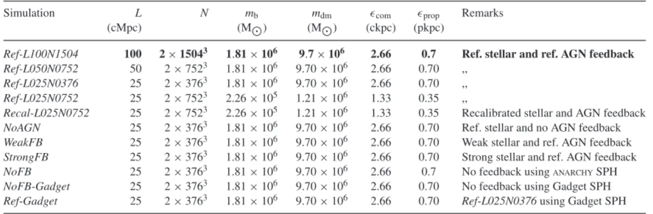
Table 1. List of cosmological simulations used in this work. The first four simulations use model ingredients identical to the EAGLE reference simulation of Schaye et al. (2015), while the higher-resolutionRecal-L025N0752has been re-calibrated to the observed present-day galaxy mass function. ModelNoAGNdoes not include AGN feedback,WeakFBandStrongFBuse half and twice as strong stellar feedback compared to the reference simulation, respectively (see Crain et al.2015). ModelsNoFBandNoFB-Gadget, do not include any feedback from stars or AGN. While the former usesANARCHY(Dalla Vecchia, in preparation) for the hydrodynamical calculations,
the latter uses the standardGADGET-3 implementation (Springel2005), as does modelRef-Gadget. From left to right the columns show:
simulation identifier; comoving box size; number of particles (there are equally many baryonic and dark matter particles); initial baryonic particle mass; dark matter particle mass; comoving (Plummer-equivalent) gravitational softening; maximum physical softening, and a brief description.
Simulation L N mb mdm com prop Remarks
(cMpc) (M) (M) (ckpc) (pkpc)
Ref-L100N1504 100 2×15043 1.81×10⁶ 9.7×10⁶ 2.66 0.7 Ref. stellar and ref. AGN feedback Ref-L050N0752 50 2×7523 1.81×10⁶ 9.70×10⁶ 2.66 0.70 ,,
Ref-L025N0376 25 2×3763 1.81×10⁶ 9.70×10⁶ 2.66 0.70 ,,
Ref-L025N0752 25 2×7523 2.26×10⁵ 1.21×10⁶ 1.33 0.35 ,,
Recal-L025N0752 25 2×7523 2.26×10⁵ 1.21×10⁶ 1.33 0.35 Recalibrated stellar and AGN feedback NoAGN 25 2×3763 1.81×10⁶ 9.70×10⁶ 2.66 0.70 Ref. stellar and no AGN feedback WeakFB 25 2×3763 1.81×10⁶ 9.70×10⁶ 2.66 0.70 Weak stellar and ref. AGN feedback
StrongFB 25 2×3763 1.81×10⁶ 9.70×10⁶ 2.66 0.70 Strong stellar and ref. AGN feedback
NoFB 25 2×3763 1.81×10⁶ 9.70×10⁶ 2.66 0.7 No feedback using
ANARCHYSPH
NoFB-Gadget 25 2×3763 1.81×10⁶ 9.70×10⁶ 2.66 0.70 No feedback using Gadget SPH
Ref-Gadget 25 2×3763 1.81×10⁶ 9.70×10⁶ 2.66 0.70 Ref-L025N0376using Gadget SPH
the observed HICDDF (Rahmati et al.2013a) andz∼3 metal
ab-sorption lines (Aguirre et al.2008). However, we emphasis that both observational constraints and model predictions for the am-plitude (UVB) and spectral shape of the photoionizing background are uncertain by a factor of a few (e.g. Faucher-Gigu`ere et al.2008,
2009; Haardt & Madau2012; Becker & Bolton2013), which could change the HIcolumn density distribution. Where appropriate, we
consider the impact of those uncertainties on our results by varying the UVB model in our calculations.
At very low HIcolumn densities, where the gas is highly ionized
the gas satisfies the so-called optically-thin limit. As the HIcolumn
density increases and its corresponding optical depth gets close to unity, photon absorptions become more important and eventually the gas can shield itself against the incoming flux of ionizing pho-tons. To account for this self-shielding, we use the same approach as we adopted in Rahmati & Schaye (2014). Namely, we use the fitting function presented in Rahmati et al. (2013a) for calculating the photoionization rate and hence the ionization state of hydro-gen atoms. This fitting function accurately reproduces the result from radiative transfer simulations of the UVB and recombination radiation in cosmological density fields usingTRAPHIC(Pawlik & Schaye2008,2011; Raiˇcevi´c et al.2014). One can characterize the UVB at any given redshift by the hydrogen photoionization rate in optically-thin limit,UVB, z, and the effective hydrogen absorp-tion cross-secabsorp-tion, ¯σνHI. Then the fitting function gives the effective photoionization rate,Phot, as a function of density:
Phot UVB,z =
0.98
1+
n H
nH,SSh
1.64−2.28
+0.02
1+ nH
nH,SSh −0.84
, (1)
wherenH is the hydrogen number density andnH, SShis the self-shielding density threshold predicted by the analytic model of
Schaye (2001a)
nH,SSh=6.73×10⁻³cm−3
¯
σνHI
2.49×10⁻¹⁸cm−2 −2/3
×
UVB
,z
10−12s−1 2/3
. (2)
Combining equations (1) and (2) allows us to calculate the equi-librium hydrogen neutral fraction of each SPH particle in our hy-drodynamical simulations after calculating its collisional ionization rate, which depends on the temperature, and its optically-thin re-combination rate (i.e. Case A)1which depend on both the density
and temperature (see appendix A2 of Rahmati et al.2013a). Since the temperature of star-forming gas in our simulations is defined by a polytropic equation of state that is used to limit the Jeans mass, and therefore is not physical, we set the temperature of the inter-stellar medium (ISM) particles toTISM=104K which is the typical
temperature of the warm-neutral ISM.
Noting that the covering fraction of extremely high HIcolumn
densities are negligible, we chose not to account for the formation of molecular hydrogen which is expected to be dominant only at
NHI10
22cm−2(Schaye2001b; Krumholz et al.2009; Rahmati
et al.2013a). We also neglect the impact of radiation from local sources, which is thought to become increasingly important for very high HIcolumn densities and very close to galaxies (Schaye 2006; Rahmati et al.2013b). Noting that the distribution of LLSs around the virial radii of galaxies is not strongly affected by local radiation (see Appendix B and Rahmati et al.2013b; Shen et al.
2013; Rahmati & Schaye2014) we postpone a treatment of lo-cal radiation, which is potentially important but requires complex radiative transfer simulations, to future work.
To calculate HIcolumn densities, we use SPH interpolation and
project the HIcontent of desired regions, which can range from the
1Note that the impact of recombination radiation is accounted for by the
full simulation box to only a small volume around a galaxy, on to a 2D grid. We found that using a grid with 10 0002=108pixels
for projecting the full box of theRef-L100N1504simulation results in converged HIcovering fractions forNHI10
22cm−2, which is
the range of HIcolumn densities we study in this work. We use 16
slices with equal widths for calculating the HIcolumn densities in
the full 100 Mpc simulation box. This enables us to calculate HI
column densities as low asNHI∼1015cm−2without being affected
by projection effects. Moreover, this choice enables us to calculate the covering fraction of HIaround simulated galaxies in analogy
with what is done observationally, where absorbers are considered to be around a galaxy only if their line-of-sight (LOS) velocity differences from that of the galaxy do not exceed a fixed value.2
Splitting the full 100 cMpc simulation box into 16 slices results in a velocity width few times smaller than the typical velocity cuts used in observational studies (e.g.V≈400 km s−1atz∼2 for each
slice). Adding together appropriate number of slices allows us to efficiently calculate the distribution of HIaround galaxies by using
velocity cuts comparable to what is typically used in observational studies (e.g. Rudie et al.2012; Prochaska et al.2013a,b).
In previous theoretical studies, the covering fraction of HIwas
usually measured by considering a finite region around galaxies which is often normalized to the virial radius of each galaxy (e.g. Faucher-Gigu`ere & Kereˇs2011; Fumagalli et al.2011,2014; Shen et al. 2013; Faucher-Gigu`ere et al. 2015). The covering fractions measured using this method only account for the gas that is much closer to galaxies along the LOS compared to what is measured observationally. Observations take into account a much longer path-length along the LOS compared to the virial radii of galaxies and are therefore not directly comparable to the covering fractions reported in previous theoretical studies. However, considering a finite region normalized to the virial radius of each galaxy is a sensible choice to study the distribution of gas that has a close physical connection to galaxies. For this reason, and also to facilitate comparison between our results and previous theoretical work, we not only mimic the observed velocity cuts, but also measure the covering fraction of HIsystems around galaxies by considering only absorbers that are
within 2×r200from each galaxy.
3 R E S U LT S
3.1 Cosmic distribution of HI
Before studying the distribution of HIaround simulated galaxies,
we need to test whether the EAGLE simulation reproduces the observed cosmic distribution of strong HIsystems. If the simulation
fails to satisfy the existing constraints on the cosmic abundance of HIabsorbers, then it is hard to trust the predictions drawn from it
about the distribution of HIclose to galaxies. While performing this consistency check is not straightforward for studies that use zoom simulations, using a cosmological simulation enables us to do so.
The cosmic HIdistribution is often quantified as the HICDDF.
The HICDDF,f(NHI, z), is conventionally defined as the number of
absorbers per unit column density, dNHI, per unit absorption length,
dX= dz(H0/H(z))(1 +z)2, and is measured observationally by
searching for HI absorbers in the spectra of background quasars
(e.g. Kim et al.2002, 2013; P´eroux et al.2005; O’Meara et al.
2007, 2013; Noterdaeme et al. 2009, 2012; Prochaska & Wolfe
2The typical velocity difference cut often used in observational studies is
>±1000 km s−1(e.g. Rudie et al.2012; Prochaska et al.2013a,b).
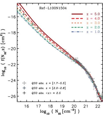
Figure 1. CDDF of neutral gas at different redshifts for theRef-L100N1504 EAGLE simulation. The data points represent a compilation of various quasar absorption line observations at high redshifts (i.e.z=[1.7, 5.5]) taken from P´eroux et al. (2005) withz=[1.8, 3.5], O’Meara et al. (2007) with
z=[1.7, 4.5], Noterdaeme et al. (2009) withz=[2.2, 5.5] and Prochaska & Wolfe (2009) withz=[2.2, 5.5]. The grey diamonds atNHI>1020cm−2
represent the most recent constraints on the high end of the HICDDF which
are taken from Noterdaeme et al. (2012) withz =2.5. The grey star-shaped data points atNHI<1017cm−2are taken from Rudie et al. (2013)
withz=[2.0, 2.8]. The simulation results are in good agreement with the observations.
2009; Prochaska, Worseck & O’Meara2009; Rudie et al. 2013; Zafar et al.2013). In Fig.1, we compare the HICDDF predicted by
theRef-L100N1504simulation with a compilation of observational results.3The predicted H
ICDDF is shown using different colours
and line styles for different redshifts ranging from z= 1 to 5. For comparison, the grey data points show the observed HICDDF forNHI10
17cm−2atz∼2–3 from Rudie et al. (2013), and at
higherNHIa compilation containing various observations spanning
the redshift range of 1.7< z <5.5 (P´eroux et al.2005; O’Meara et al.2007; Noterdaeme et al.2009; Prochaska & Wolfe2009). The most recent measurements of the HICDDF at very highNHIand
an average redshift ofz =2.5 from Noterdaeme et al. (2012) are also shown using dark grey diamonds.
Fig. 1 shows that there is good agreement between the pre-dicted HICDDFs and observations for strong HIabsorbers (NHI
1019cm−2), similar to what was found for OWLS (Altay et al.2011;
Rahmati et al.2013a). The weak evolution of the high end of the HI
CDDF that we reported for OWLS in Rahmati et al. (2013a) is also evident. However, we note that the measurements of Rudie et al. (2013) for the CDDF are slightly underproduced by our simulation which indicates the need to use a lower hydrogen photoionization rate atz=2.5 compared to what our fiducial UVB model implies
3We apply appropriate corrections for the different cosmological
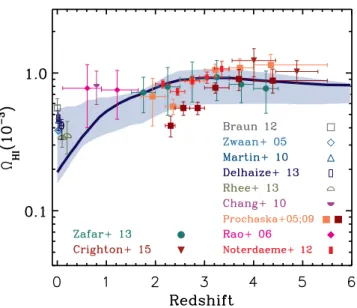
Figure 2. Cosmic density of HI as a function of redshift in the
Ref-L100N1504EAGLE simulation (solid curve). The shaded area around the curve indicates the range covered by all the simulations listed in Table1
(expect models with no feedback). The data points represent a compilation of various quasar absorption line observations taken from Rao, Turnshek & Nestor (2006) withz=[0.11–1.65], Prochaska, Herbert-Fort & Wolfe (2005), Prochaska & Wolfe (2009) withz=[2.2, 5.5], Noterdaeme et al. (2012) withz=[2.0, 3.5], Zafar et al. (2013) withz =[1.5, 5.0] and Crighton et al. (2015). The low-redshift compilation of data is based on 21-cm emission studies of Zwaan et al. (2005), Martin et al. (2010), Braun (2012) and Delhaize et al. (2013) atz∼0, stacked 21-cm emission studies of Rhee et al. (2013) atz∼0.1–0.2 and 21-cm intensity mapping of Chang et al. (2010) atz≈0.8.
(see Appendix A). It should also be noted that because we do not correct the simulation for H2, the agreement atNHI1022cm−2
may be fortuitous.
The cosmic HIdensity,HI, which is defined as the mean HI
density divided by the critical density,ρcrit, can be calculated either by estimating the observed HImass density through HI21-cm
emis-sion at low redshifts or by integrating the HICDDF of absorbers at high redshifts:
HI= H0mH
cρcrit ∞
0
NHIf(NHI, z)dNHI, (3)
whereH0=100 hkm s−1Mpc−1is the Hubble constant,mHis
the mass of a hydrogen atom,cis the speed of light and ρcrit= 1.89×10⁻²⁹h2g cm−3.
The predicted evolution of the cosmic HIdensity for the Ref-L100N1504EAGLE simulation is shown with the solid curve in Fig.2. The shaded area around the curve shows the range covered by the other feedback enabled simulations we use in this work (see Table1). For comparison, a compilation of various observational measurements are overplotted with different symbols. The high-z (z1) measurements of theHIare often based on the observed
abundance of DLAs4(e.g. Prochaska et al.2005; Rao et al.2006;
Prochaska & Wolfe2009; Noterdaeme et al.2012; Zafar et al.2013). The low-redshift measurements are generally based on measuring the HImass using 21-cm emission and often involve adopting
non-4Note that due to the shape of the H
ICDDF, the cosmic HIdensity is very
sensitive to the abundance of DLAs and that the contribution of lowerNHI
systems is negligible.
trivial assumptions about the HIgas fraction of the full galaxy
population to derive the cosmic HIdensity (e.g. Zwaan et al.2005;
Chang et al.2010; Martin et al.2010; Delhaize et al.2013; Rhee et al.2013). The comparison between the predicted and observed
HIshows good agreement, particularly at the redshifts of interest
here,z >1. While the cosmic HIdensity remains nearly constant
fromz∼6 toz∼ 2–3, it declines towards lower redshifts. This decline, which is also evident in observed evolution of theHI,
is not reproduced in some previous theoretical studies (e.g. Dav´e et al.2013; Lagos et al.2014). The cosmic HIdensity in the Ref-L100N1504simulation seems to drop faster than observed, while the range of predictions obtained by varying the resolution and/or box-size of the simulation (shaded region around the solid curve in Fig.2) is fully consistent with the observational measurements at
z≈0. Moreover, as we mentioned above, it is important to note that measurements ofHIat low redshift often involve strong
assump-tions about the HImass fractions of all galaxies and are therefore not as robust as the direct measurements at higher redshifts.
Having shown that the observed cosmic distribution of HI is
reproduced reasonably well, we can use the simulation with more confidence to study the HIdistribution around galaxies.
3.2 Covering fraction of LLSs inside haloes
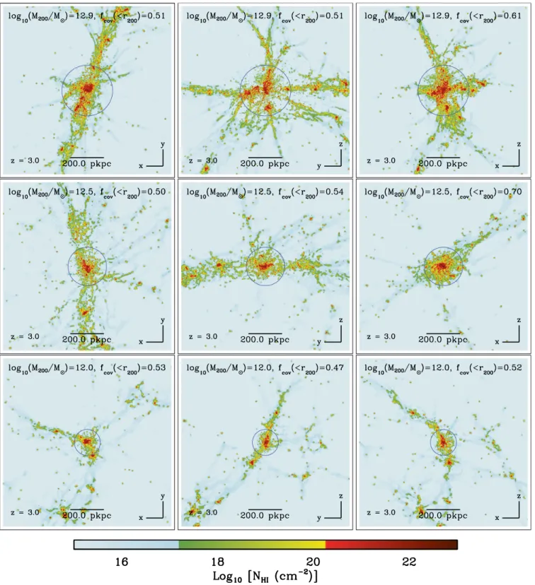
Examples of the distribution of HIaround simulated galaxies at z=3 are shown in Fig.3. In this figure, the coloured maps show the HIcolumn density distributions in 1×1 pMpc2regions centred on
galaxies withM200=1012–1013M
. The virial radius,r200, of each galaxy is shown with a blue circle and each galaxy map is shown using three different orthogonal projections. A significant fraction of the area within the virial radii of massive galaxies is covered with LLSs (i.e.NHI>10
17.2 cm−2) which have highly inhomogeneous
distributions with often form filamentary structures. As a result, the fraction of the area covered by LLSs inside the virial radius, which is indicated in the top-right corner of each panel, varies depending on the point of view and from one galaxy to another. However, the average LLSs covering fraction does not depend strongly on the halo mass. On the other hand, as Fig.4shows, the typical LLSs covering fraction decreases significantly fromz=4 to 2.
To quantify the distribution of HIaround galaxies, the covering
fraction of LLSs within the virial radius,f<r200, is defined as the probability of finding systems withNHI>10
17.2cm−2with impact
parameters smaller than the virial radius,r200 and with LOS dis-tances from the galaxy shorter than a specific value comparable to the virial radius. Equivalently,f<r200can be defined as the fraction of the surface area withinR<r200that is covered by LLSs after projecting the gas distribution within a specific LOS distance from the galaxy on to a 2D plane. We calculate this quantity for each galaxy by projecting the HIwithin a slice with 4×r200thickness
centred on the galaxies redshift5and repeating the same calculation
for projections along three different orthogonal directions. Then we calculatef<r200by measuring the fraction of the surface contained within ther200that is covered by LLSs.
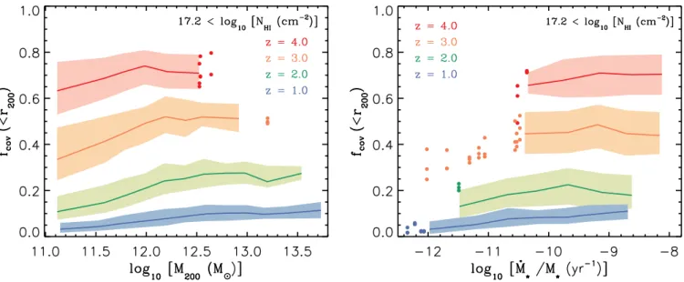
The predictedf<r200for different redshifts is shown in Fig.5as a function of halo mass,M200, in the left-hand panel, and as a function of specific star formation rate, ˙M/M, in the right-hand panel. Each solid curve and the shaded area around it show, respectively, the
5We used this definition to be consistent with previous studies (e.g.
Figure 3. The simulated HIcolumn density distribution around randomly selected massive galaxies atz=3. Top, middle and bottom rows show galaxies
withM200≈1012,≈1012.5and≈1013M, respectively. The columns in each row show a single galaxy as seen from three different orthogonal angles. Blue
circles are centred on galaxies and show the virial radii (i.e.r200). Each panel shows a 1×1 pMpc2region with the same projected depth. The covering fraction
of LLSs (i.e.NHI>1017.2 cm−2) with impact parameters less thanr200is indicated in the top-right of each panel. Atz=3, LLSs (green regions) form
filamentary structures and their distribution varies strongly from galaxy to galaxy, and with the viewing angle. The typical covering fraction of LLSs within r200does not vary strongly with halo mass at a given redshift.
median covering fraction and the corresponding 15–85 percentiles for theRef-L100N1504simulation. In this figure, red, orange, green and blue curves showz=4, 3, 2 and 1, respectively. For massive haloes withM2001012M
,f<r200 does not depend strongly on
halo mass. For less massive haloes (i.e.M2001012M
Figure 4. The same as Fig.3but for galaxies withM200≈1012.5Mat redshiftsz=4, 3 and 2 (from top to bottom, respectively). The columns in each
row show a single galaxy as seen from three different orthogonal angles. LLSs (green regions) form filamentary structures at all redshifts, which become less prominent by decreasing redshift. The typical covering fraction of LLSs withinr200evolves rapidly with redshift.
While the dependence of f<r200 on halo mass is rather weak,
the covering fractions increase strongly with redshift. This result is consistent with haloes containing increasingly higher gas fractions at higher redshifts as a result of increasing rates of cold accretion and the higher mean density of the Universe. As we will show in Section 3.3, this weak halo mass dependence enables us to
Figure 5. Cumulative covering fraction of LLSs withinr200as a function of halo mass,M200(left) and specific star formation rate, ˙M/M(right). Curves from top to bottom show redshiftsz=4 (red), 3 (orange), 2 (green) and 1 (blue). Solid curves show the median covering fractions for theRef-L100N1504 simulation and the shaded areas around them indicate the 15–85 percentiles. Galaxies are shown with individual data points instead of curves in bins that contain fewer than 10 galaxies. About 35 000 galaxies (each in three different orientations) were used to make this figure. The covering fraction increases strongly with redshift for all halo masses. It also increases with halo mass but this dependence is weak for massive objects. There is no strong correlation between the covering fraction of LLSs and the specific star formation rate.
finding LLSs within a given distance from galaxies does not repre-sent the covering fraction of LLSs at the typical (e.g. mean) redshift of the galaxy sample, because higher redshift galaxies have larger contributions to the average covering fraction of the population. As we will discuss in Section 4, together with other biases like the wide range of halo masses represented by observational samples, this issue can explain the large covering fractions derived from some observational samples (e.g. Prochaska et al.2013b).
The right-hand panel of Fig.5shows thatf<r200 does not
de-pend strongly on the specific star formation rate of galaxies.6Only
galaxies withM200>1011.5M
are shown in the right-hand panel of Fig. 5, but our experiments show that a narrow range of halo masses only strengthens the independence off<r200 from the spe-cific star formation rate. This trend thus suggests that the covering fraction of LLSs does not depend strongly on the transient varia-tions in the star formation activity of galaxies, and is set by their average star formation activity and the large-scale distribution of gas around them.
As the shaded areas around the median curves in Fig.5illustrate, there is significant scatter in the predicted covering fraction at any given mass and specific star formation rate. This scatter is larger at higher redshifts where the typical covering fractions are also larger. We note that the covering fraction of a single simulated galaxy can change from one projection axis to another by a factor close to the typical scatter for its mass range (see Fig.3), which is consistent with what Fumagalli et al. (2014) found. This, together with the lack of strong dependence between the covering fraction and specific star formation rate, suggests that most of the scatter shown in Fig.5can be attributed to the highly inhomogeneous and filamentary distribution of HIaround galaxies.
6Note that we neglect the impact of local sources onf
<r200. If local sources were to change thef<r200significantly, then they could introduce a depen-dence on the specific star formation rate.
Although f<r200 is widely used to quantify the distribution of HIaround galaxies, both in theoretical and observational studies, one should note that the virial radius is not a directly observable quantity. Moreover, as mentioned above, the virial radius of a sam-ple of galaxies with a wide range of different characteristics (e.g. mass, redshift) is not well defined. For this reason, we opted not to compare the covering fractions shown in Fig.5with those re-ported in observational studies (e.g. Rudie et al.2012; Prochaska et al.2013a,b). Instead, we compare to observations after matching the redshift and halo mass distribution of observed and simulated samples in Section 4.
3.3 Covering fraction profiles
In the previous section, we studied the cumulative covering fraction of LLSs within the virial radius (i.e.f<r200). However, more infor-mation is embedded in the differential covering fraction profile of HIabsorbers with different column densities as a function of
im-pact parameter from galaxies. We define the differential covering fraction in a given impact parameter bin as
fcov(R)≡fcov(Ri< R < Ri+1)≡
Aabs|Ri+1
Ri
π(R2
i+1−Ri 2
), (4)
whereAabsis the area covered by absorbers (e.g. LLSs) within a radial bin defined by the impact parametersRiandRi+1, assuming
thatRi+1 >Ri> 0. Note that throughout this work, we reserve
fcov(R) the differential covering fraction andfcov(<R) for the cu-mulative covering fraction (e.g. Figs5and10). For instance, we denote the cumulative covering fraction within an impact parameter equal to the virial radius byf<r200=fcov(0< R < r200) as shown in Fig.5.
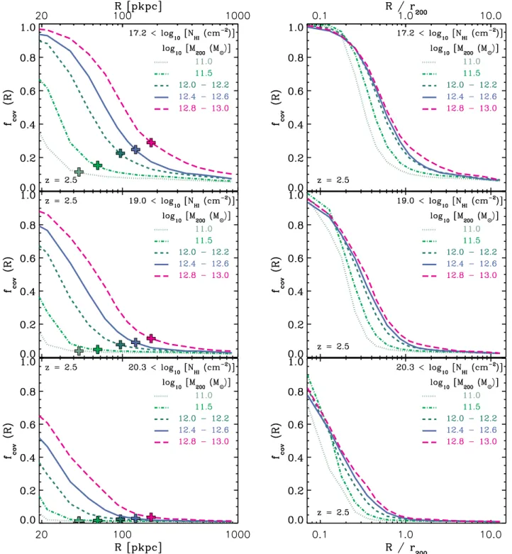
Figure 6. Profiles showing the mean differential covering fraction of LLSs (top), sub DLAs (middle) and DLAs (bottom) as a function of impact parameter (left) and normalized impact parameter (right) for different halo mass bins in theRef-L100N1504EAGLE simulation atz=2.5 usingV=3150 km s−1. In
the left-hand panel, the virial radius corresponding to each halo mass bin is indicated with a cross. As the left-hand panels show, all covering fractions depend strongly on halo mass at fixed impact parameters, particularly very close to galaxies. The right-hand panels show, however, that only a weak mass dependence remains in the covering fraction profiles of haloes withM2001012M, after normalizing the impact parameters to the virial radii. This suggests that the
shape of the covering fraction profiles of LLSs, sub DLAs and DLAs is similar in all haloes withM2001012Mand the mass dependence of the covering
fractions at fixed physical impact parameters stems mainly from the differences in the halo sizes.
around each galaxy a velocity window ofV=3150 km s−1(i.e.
the allowed velocity difference between absorbers and galaxies is
≤±1575 km s−1) is adopted for calculating its covering fraction, but
we note that increasing or decreasing the allowed velocity width by a factor of a few does not change the results forR<r200(see Fig.C1).
The five mass bins shown in the top-left panel of Fig.6have similar LLSs covering fractions at the outermost impact parameters, but they vary strongly with halo mass close to galaxies. As the middle-left and bottom-middle-left panels in Fig.6show, the same qualitative trend holds for sub DLAs (i.e.NHI>10
increasing the HIcolumn density of absorbers, the covering fraction
at fixed impact parameters decreases. Despite the sensitivity of the covering fractions to the halo mass, it seems that the shapes of the curves are very similar for halo massesM200 1012M
which suggests that they can be matched by a re-scaling to account for differences in the virial radii of the haloes.
To show that the covering fraction profiles are nearly scale in-variant, we normalize the impact parameters to the virial radii of the haloes in the panels of the right-hand side of Fig.6. The good agreement between the three curves that representM2001012M
haloes shows that the covering fraction profiles of LLSs, sub DLAs and DLAs around those haloes are self-similar with a characteristic scalelength very close to the virial radius. This is the main reason behind the very weak dependence of the total LLS covering fraction withinr200(f<r200) and halo mass for galaxies withM20010
12M
(see Fig.5). As the curves for the two lowest mass bins in the right-hand panels of Fig. 6show, the scale-invariance of the covering fraction profiles breaks down for galaxies withM200<1012M
, where the total covering fraction of absorbers withinr200also slowly decreases with decreasing halo mass (see Fig.5).
The scale-invariance of the distribution of strong HIabsorbers
around massive haloes allows us to calculate the typical normal-ized covering fraction profiles that characterize the distribution of LLSs, sub DLAs and DLAs around haloes withM2001012M
at any given redshift.7 Based on the strong evolution of the
to-tal HIcovering fraction inside haloes (see Fig.5), it is expected
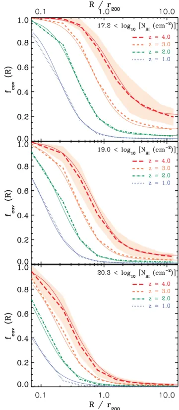
that the normalized covering fraction profiles also evolve strongly with redshift. To illustrate this, we show the normalized differential covering fraction for LLSs, sub DLAs and DLAs in, respectively, the top, middle and bottom panels of Fig.7. The different curves in each panel indicate different redshifts where long-dashed (red), dashed (orange), dot–dashed (green) and dotted curves showz=4, 3, 2 and 1, respectively. Note that a LOS velocity window of width
V=3000 km s−1is adopted for calculating the covering fractions
shown in this figure. To illustrate the typical intrinsic scatter in the covering fraction profiles, the 15–85 percentiles of the covering fractions at z= 4 are indicated by the shaded areas around the long-dashed red curves. The normalized covering fraction profiles of all strong HIabsorbers indeed evolve strongly.
Definingx ≡ R/r200 as the normalized impact parameter, the covering fraction of HI absorbers around galaxies with a given
virial radius, r200, at redshiftz can be fitted with the following function:
fcov(x, z)=1− 1 1+ Lzx
α + C
⎡ ⎢
⎣ 1
1+ Lzx
3 ⎤ ⎥
⎦10z−34, (5)
whereLzis a redshift-dependent characteristic length scale that is given by
Lz=A Bz, (6)
andA,B,Candαare free parameters that vary for LLSs, sub DLAs and DLAs. Based on this fitting function, the covering fraction approaches unity very close to galaxies wherexLzand at very high redshifts wherez→ ∞. However, note that the latter is the case only ifB< 101/6. Far from galaxies wherexL
z, on the
other hand, the covering fraction approaches the asymptotic value ofC10z−34.
7TheRef-L100N1504EAGLE simulation contains 95, 345, 824 and 1436
haloes withM2001012Mat redshiftsz=4, 3, 2 and 1, respectively.
Figure 7. Normalized differential covering fraction profiles of HIabsorbers
around galaxies withM200 ≥1012M in theRef-L100N1504 EAGLE
simulation at different redshifts usingV=3000 km s−1. The top, middle
and bottom panels show the covering fractions of LLSs, sub DLAs and DLAs, respectively. The red (long-dashed), orange (dashed), green (dot– dashed) and blue (dotted) curves show the results atz =4, 3, 2 and 1, respectively, while the thin solid curves show the fitting function given by equations (5) and (6). The covering fractions for stronger HIabsorbers
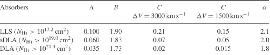
Table 2. The best-fitting values for the free parameters of the fitting function, equations (5) and (6), for the predicted normalized covering fraction of LLSs, sub DLAs and DLAs for haloes with M200 ≥1012Mat redshiftsz4. Note that parameterCis sensitive to the chosen velocity
width and is reported for two velocity widthV=3000 and 1500 km s−1. The performance of
the fitting function (thin solid curves) is shown in Fig.7forV=3000 km s−1.
Absorbers A B C C α
V=3000 km s−1 V=1500 km s−1
LLS (NHI>1017.2cm2) 0.100 1.90 0.21 0.15 2.1
sDLA (NHI>1019.0cm2) 0.060 1.83 0.07 0.05 2.0
DLA (NHI>1020.3cm2) 0.035 1.73 0.02 0.015 1.8
Table2lists the best-fitting values for the free parameters. As shown in Appendix C, the covering fraction of absorbers at relatively large impact parameters (R>r200) is sensitive to the size of the LOS velocity window that is used for associating HI absorbers
and galaxies. As a result, parameterCin the fitting function of equation (5) is sensitive to the adopted velocity width. Therefore, we report two sets of best-fitting values ofCwhere each set corresponds to eitherV=3000 km s−1orV=1500 km s−1.
As the thin solid curves in Fig.7show, the predicted normal-ized covering fraction profiles are all closely matched by the values obtained from equation (5) for appropriate choices of the free pa-rameters that are listed in Table2. We note that the differences between the fitting formula and the simulation are much smaller than the typical intrinsic scatter in the covering fractions, which are shown in Fig.7forz=4 by the shaded areas around the long-dashed red curves. Note that variations in the assumed UVB radiation can change the covering fraction of LLSs. For instance, reducing the UVB photoionization rate by a factor of 3 results in LLS covering fractions that are higher by∼0.1. However, such moderate changes in the UVB do not significantly affect the distribution of highly self-shielded stronger absorbers such as sub DLAs and DLAs.8
The values of the free parameters that control the empirical fit-ting function that we introduced above are physically meaningful. For instance,Lzcould be regarded as a typical projected distance between absorbers and galaxies. Taking the values ofAandBfrom Table2, the implied typical projected distances between LLSs, sub DLAs and DLAs and their host galaxies atz≈3 are, respectively,
≈r200,≈0.5r200and≈0.2r200, which is in excellent agreement with the predictions of Rahmati & Schaye (2014) from the OWLS simu-lations (see the right-hand panel of their fig. 3). Moreover, equation (6) implies that the typical normalized impact parameter of strong HIabsorbers increases exponentially with redshift. The best-fitting
values forB, which controls the rate of this change, imply that the impact parameters of LLSs evolve slightly faster than those of DLAs. Moreover, the higherαvalue for LLSs indicates that their covering fractions drop faster than those of DLAs with increasing normalized impact parameters.
The rightmost term in equation (5) is related to the contribution of the background absorbers outside of the halo. Given the steep HI
CDDF (see Fig.1), there are many more LLSs than DLAs. Given the fixed LOS velocity cut imposed to obtain the covering fraction of absorbers, one would expect the ratio between the covering fraction of absorbers at large virial radii to follow the ratio between their cosmic abundances. As the best-fitting values for theCparameter
8It is important to keep in mind that very close to galaxies (Rr 200) the
predicted covering fractions may be overestimates because we neglect local sources of ionizing radiation.
imply, this is indeed the case (e.g. LLSs are∼10 times more frequent than DLAs at all redshifts).
We note that local sources of ionizing radiation, which we have ignored, may cause the fitting function to underpredict the covering fraction of strong HIabsorbers close to galaxies (see Appendix B). We emphasize that we only considered the redshift range 1≤z≤4 when deriving our fitting function. While the same function pro-duces a reasonable match to the simulated normalized HIcovering
fractions atz=5 forRr200, it predicts LLS covering fractions that are≈10 per cent too high for larger impact parameters. This difference is smaller than (but comparable to) the intrinsic scatter (i.e. 15–85 percentiles) in the simulated normalized profiles.
4 C O M PA R I S O N W I T H O B S E RVAT I O N S
Recent observations found large covering fractions of LLSs close to massive haloes atz∼2 (Rudie et al.2012; Prochaska et al.2013a,b) which implies the existence of a large reservoir of neutral and hence relatively cold gas around massivez∼2 galaxies. However, recent simulations of∼1012.5M
haloes at z∼ 2 by Fumagalli et al. (2014) and Faucher-Gigu`ere et al. (2015) resulted in LLSs covering fractions that are much smaller than observed by Prochaska et al. (2013b). This discrepancy may indicate that our current theoretical understanding of galaxy formation and evolution is inadequate.
The EAGLE simulation is ideal to revisit this problem since its volume is sufficiently large to contain a large number of haloes with
M2001012M
atz∼2–3 without compromising the resolution needed to reproduce the observed cosmic distribution of HI(see
Section 3.1). Because of the large intrinsic scatter in the covering fractions, a large sample of simulated galaxies is required to con-strain the average covering fraction at any given mass. Moreover, thanks to efficient stellar and AGN feedback, EAGLE reproduces the basic observed characteristics of galaxies over wide ranges of mass and redshift (S15; Furlong et al.2015). In addition, using a large cosmological simulation enables us to calculate the HI
cover-ing fractions for a LOS path length comparable to what is typically used in observational studies.
In the following, we compare EAGLEs predictions with the ob-servational constraints on the distribution of HIaround massive
star-forming galaxies (Rudie et al.2012) and quasars (Prochaska et al.2013b) atz∼2.
4.1 HIdistribution around quasars atz∼2
Prochaska et al. (2013a,b) observed the distribution of HI
around bright quasars at z ∼ 2. Clustering analysis indicate that those quasars which typically reside in massive haloes with
M200∼1012.5M
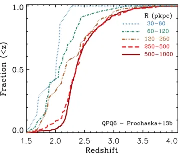
Figure 8. Cumulative redshift distribution of the foreground quasars from the QPQ6 sample (Prochaska et al.2013b). Different curves show the red-shift distribution of foreground quasars in different impact parameter bins, identical to those used in Fig.9. Most quasars are at large impact parame-ters and have a wide range of redshifts, extending up toz4. More than 30 per cent of quasars withR100 pkpc have redshiftsz2.5. Given the rapid increase of the HIcovering fraction with redshift that we found in this work, those quasars can strongly bias the estimated covering fraction of LLSs, particularly at large impact parameters. Moreover, for a magnitude-limited survey, higher-redshift quasars are likely to reside in more massive haloes which may further bias the estimated covering fractions at fixed impact parameters.
sample of foreground quasars (hereafter the QPQ6 sample), Prochaska et al. (2013b) measured the covering fraction of LLSs in different impact parameter bins. Adopting a fixed typical halo mass of 1012.5M
atz∼ 2, and consequently a fixed virial radius of 160 kpc for all quasars in the QPQ6 sample, Prochaska et al. (2013a) concluded that more than60 per cent of the area within the virial radii of haloes with masses around 1012.5M
atz∼2 is covered by LLSs. For their covering fraction measurement, Prochaska et al. (2013a) adopted a velocity width ofV=3000 km s−1to associate
absorbers to quasars.
For a proper comparison between our simulation and the obser-vations of Prochaska et al. (2013a,b), it is important to note that the foreground quasars in the QPQ6 sample have a relatively wide range of bolometric luminosities. Since quasars are variable, a one-to-one relation between quasar luminosity and halo mass is not expected. However, as a rough estimate, if we assume a positive correlation between the halo mass of galaxies and the bolometric luminosity of the quasars, we could conclude that quasars in the QPQ6 sample represent a relatively wide range of halo masses some of which could well exceed the typical halo mass ofM200∼1012.5M
. If the host haloes of the observed quasars indeed have a range of masses, then the adopted fixed virial radius of 160 pkpc for calculating the total covering fraction of LLSs inside the virial radii of haloes with
M200≈1012.5M
atz≈2 could result in an overestimate of the true covering fraction due to the non-negligible contribution of haloes withM200>1012.5M
in the QPQ6 sample.
It is also important to note that the foreground quasars in the QPQ6 sample are not all at the same redshift. In addition, as Fig.8
shows, there is a systematic trend between the typical redshift of foreground quasars and the impact parameter at which their gas content is measured. As a result, the typical redshift of quasars
for the smallest impact parameters (∼10–100 pkpc) isz≈2 but it increases toz≈2.5 for impact parameters∼1 pMpc. The high-ztail of the distribution for quasars with impact parametersR100 pkpc is quite extended and more than 30 per cent of them havez >2.5. Given our finding that the HIdistribution around galaxies atz∼2–3
evolves rapidly, this systematic bias should be taken into account when comparing simulations with observations.
In addition, the HIdistribution is sensitive to the intensity of the UVB radiation. However, observational constraints on the intensity of the UVB at 2z6 are model dependent and uncertain by a factor of a few (e.g. Bajtlik, Duncan & Ostriker1988; Rauch et al.
1997; Bolton et al.2005; Faucher-Gigu`ere et al.2008; Calverley et al.2011; Becker & Bolton2013). UVB models are also uncertain due to the various assumptions they need to adopt (e.g. the escape fraction of ionizing photons into the IGM, mean-free-path of ion-izing photons, abundance of faint sources) and differ from each other by a factor of a few (e.g. Haardt & Madau2001; Faucher-Gigu`ere et al.2009; Haardt & Madau2012). While the intensity of our fiducial UVB model (i.e. Haardt & Madau2001) is well within the range of the most recent estimates (e.g. Becker & Bolton
2013), intensities lower by up to a factor of∼3 are consistent with some observations/models atz∼2–3 (e.g. Faucher-Gigu`ere et al.
2008,2009; Haardt & Madau2012), and would further improve the agreement between EAGLE and the observed HIcolumn density distribution belowNHI≈10
17cm−2(see Fig.1).
It is necessary to take the aforementioned considerations into ac-count when comparing simulations and observations. To do this, we calculate the covering fraction of LLSs around simulated galaxies withM200>1012.5M
in theRef-L100N1504simulation atz=2.2 and 3, resulting in 116 and 39 haloes,9respectively, with a median
mass ofM200 =1012.6M
.10 The two selected redshifts bracket
the range of redshifts that is represented by the QPQ6 sample. As shown in Appendix A, varying the UVB model changes the result-ing HIcovering fraction. It is therefore important to include also
the uncertainties in the amplitude of the UVB photoionization rate. To do this, we calculate the HIdistributions using both our fiducial
UVB model of Haardt & Madau (2001) and the Haardt & Madau (2012) UVB model. Noting that atz≈3 the latter yields a hydro-gen photoionization rate≈3 times weaker than for our fiducial UVB model, we consider thez=3 HIcovering fractions calculated using the Haardt & Madau (2012) model upper limits on the predictions. Given the steep evolution in the HIcovering fractions fromz=3 to
2, we use the simulation results atz=2 that use our fiducial Haardt & Madau (2001) UVB model as lower limits for the predictions. Then, we calculate the covering fraction of LLSs, sub DLAs and DLAs for each halo using impact parameter bins identical to the analysis of Prochaska et al. (2013b). We use a LOS velocity win-dow ofV=3000 and 3400 km s−1around each galaxy atz=2.2
9Although the number of simulated haloes we use is less than the observed
number (155 simulated haloes versus 646 observed quasars), we use∼105
sight-lines per simulated object to calculate the covering fraction profiles. In other words, we use∼107sight-lines to calculate the predicted HI
distri-butions that are shown in Fig.9while only≈600 observed sight-lines are used in Prochaska et al. (2013b).
10We note that due to steepness of the mass function around the halo mass
andz=3 for calculating the covering fractions to mimic closely what is done observationally.11
The predicted covering fractions of HIabsorbers are shown in
Fig.9for LLSs (top panel), sub DLAs (middle panel) and DLAs (bottom panel). The upper and lower edges of the dark-coloured areas in each panel show the lower and upper limits of our pre-dicted mean covering fractions obtained by applying the fiducial UVB model toz=2.2 haloes and a three times weaker UVB model toz= 3 haloes, respectively. The shaded areas around the dark regions, which are shown using light colours, indicate the regions enclosed between the 15 percentiles of the lower limit for cover-ing fraction (i.e. atz= 2.2 and using the fiducial UVB model) and the 85 percentile of the upper limit for the covering fraction (i.e. atz=3 and using the weaker UVB model) in each impact parameter bin. In other words, the dark regions show how much variation is expected in the predicted covering fractions due to sys-tematic effects caused by the redshift distribution of the quasar sample and the photoionization rate of the UVB, and the light-coloured areas around the dark regions show the predicted 1σ scat-ter (15–85 percentiles) around the mean due to object-to-object variations in the covering fraction within the sample of simulated haloes.
Grey diamonds with error bars show the observations of Prochaska et al. (2013b) where the horizontal error bars show the impact parameter bins and the vertical error bars show only the 1σstatistical uncertainty. Comparing the observed data points with the predicted results shows overall good agreement for absorbers with different HIcolumn densities. The agreement is particularly
good for larger impact parameters (>60 pkpc) despite the fact that the observational error bars are smallest there owing to the larger number of quasar pairs.
For impact parameters in the range 30–60 pkpc we appear to predict too high covering fractions and for DLAs this discrepancy is marginally significant. However, given that only six of the nearly 600 observed quasar pairs fall in this bin, one may question the robustness of the error estimates. There could also be biases. For example quasars covered by DLA absorption may be missing from the bright sample because of obscuration. The theoretical prediction is also most uncertain at the smallest impact parameters. For exam-ple, radiation from local stars thought to be the dominant source of hydrogen photoionization close to galaxies (e.g. Schaye2006; Rahmati et al.2013b) and would reduce the abundance of HI(see
Appendix B). The presence of bright quasars will strengthen this ef-fect. Quantifying the impact of local radiation on our results would require detailed radiative transfer simulations that also account for the duty cycle of quasars.
The top panel of Fig.9shows the simulation predictions from Fumagalli et al. (2014) using open squares and light-red shaded areas which, respectively, show the mean and 1σ scatter for cov-ering fraction of LLSs around five simulated galaxies with halo massesM200≈1012.2M
atz=2. Their LLS covering fractions are significantly lower than both our predictions and observations. There are several potential explanations for this difference. Fuma-galli et al. (2014) analysed the HIdistribution at lower redshift and
with lower masses than the objects in the QPQ6 sample. In addition,
11Since we use slices with fixed comoving lengths to mimic the velocity
windows around galaxies, the width of the resulting velocity window be-comes redshift dependent, but remains close enough to the value used in the observational analysis.
Figure 9. Predicted and observed differential HIcovering fractions around
quasars atz≈2. The data points with error bars show the observations of Prochaska et al. (2013b) for a sample of quasar atz =2.3. Predicted mean covering fractions for haloes withM200≥1012.5Min theRef-L100N1504
Figure 10. Cumulative covering fraction of HIsystems with different column densities inside a given impact parameter,R, as a function of impact parameter for
LBGs. From top-left to the bottom-right, panels show the covering fraction of HIsystems withNHI>1015.5 cm−2,NHI>1017.2 cm−2,NHI>1019.0 cm−2
andNHI>1020.3 cm−2, respectively, and with impact parameters<R. The data points with error bars show the measurements from Rudie et al. (2012) for a
sample of LBGs withM200≈1012Matz =2.4 and 2.3 for the inner and outer impact parameter bins, respectively. Predicted mean covering fractions
for haloes with 1011.8<M
200<1012.2Min theRef-L100N1504EAGLE simulation are shown with dark-coloured regions which indicate the systematic
uncertainty in the mean due to uncertainties in the background ionizing radiation and the redshift range of the observed LBGs (see the text). The light shaded areas indicate the 15–85 percentiles for the scatter due to object-to-object variation. The predictions agree well with the observations.
the simulations analysed by Fumagalli et al. (2014) did not include the efficient feedback that, as we show in Section 5, is required to obtain reasonable stellar masses and HIcovering fractions for the
haloes they considered. Furthermore, because they used zoom sim-ulations, Fumagalli et al. (2014) only considered the distribution of absorbers with small LOS separations from the galaxies (R∼r200) when calculating covering fractions. In contrast, observations used a LOS velocity window ofV=3000 km s−1which translates into
distances much larger than the virial radii of the relevant haloes. While this difference does not affect the covering fractions at im-pact parametersRr200, it results in large differences atRr200
(e.g. up to100 per cent difference in the covering fraction of LLSs atR∼200–1000 pkpc forM200≈1012.5M
haloes atz=2.5, as shown in Fig.C1).
4.2 HIdistribution around LBGs atz∼2
In addition to quasars, there are observational constraints on the HIdistribution around star-forming galaxies atz∼2 (e.g. Rakic
et al.2012; Rudie et al.2012; Turner et al.2014). Here we compare with the data from Rudie et al. (2012), who used spectra of back-ground quasars behind a sample of LBGs atz≈2–2.5 to measure the covering fraction of HIclose to LBGs, which have halo masses M200∼1012M
(Adelberger et al.2005; Trainor & Steidel2012; Rakic et al.2013). By considering all absorbers that are within a LOS velocity window ofV=1400 km s−1around each galaxy,
Rudie et al. (2012) calculated the average covering fraction of HI