Pattern mixture models for clinical validation of biomarkers in
the presence of missing data
Fei Gaoa, Jun Dongb, Donglin Zenga, Alan Rongc, and Joseph G. Ibrahima,*
aDepartment of Biostatistics, University of North Carolina at Chapel Hill, CB7420, Chapel Hill,
U.S.A
bAmgen Inc., One Amgen Center Drive, Thousand Oaks, U.S.A cAstellas Pharma Inc., Northbrook, U.S.A
Abstract
Targeted therapies for cancers are sometimes only effective in a subset of patients with a particular biomarker status. In clinical development, the biomarker status is typically determined by an investigational-use-only/laboratory-developed test. A market ready test (MRT) is developed later to meet regulatory requirements and for future commercial use. In the USA, the clinical validation of MRT showing efficacy and safety profile of the targeted therapy in the biomarker subgroups determined by MRT is needed for pre-market approval. One of the major challenges in carrying out clinical validation is that the biomarker status per MRT is often missing for many subjects. In this paper, we treat biomarker status as a missing covariate and develop a novel pattern mixture model in the setting of a proportional hazards model for the time-to-event outcome variable. We specify a multinomial regression model for the missing biomarker statuses, and develop an expectation–maximization algorithm by the Method of Weights (Ibrahim, Journal of the American Statistical Association, 1990) to estimate the parameters in the regression model. We use Louis’ formula (Louis, Journal of the Royal Statistical Society. Series B, 1982) to obtain standard errors estimates. We examine the performance of our method in extensive simulation studies and apply our method to a clinical trial in metastatic colorectal cancer.
Keywords
clinical trials; companion diagnostics; missing data
1. Introduction
Targeted therapies for cancers are sometimes only effective in a subset of patients, restricted by one or more biomarkers. One such example is the anti-EGFr monoclonal antibodies for metastatic colorectal cancer (mCRC) patients. The targeted therapy Vectibix is currently indicated for mCRC in the wild-type KRAS population in many countries as combination
*Correspondence to: Joseph G. Ibrahim, Department of Biostatistics, University of North Carolina, Chapel Hill, NC 27599, U.S.A.,
HHS Public Access
Author manuscript
Stat Med
. Author manuscript; available in PMC 2018 August 30. Published in final edited form as:Stat Med. 2017 August 30; 36(19): 2994–3004. doi:10.1002/sim.7328.
A
uthor Man
uscr
ipt
A
uthor Man
uscr
ipt
A
uthor Man
uscr
ipt
A
uthor Man
uscr
with chemotherapy or monotherapy, while the mutant KRAS population does not benefit from Vectibix. To identify this subpopulation, an in vitro diagnostic (IVD) assay needs to be developed as a companion to the targeted therapy. This is also required by the Food and Drug Administration guidance [1] to get approval for the therapy for intended use in the biomarker subpopulation and co-approval of the IVD assay defining that subpopulation.
Ideally, the IVD assay is developed concurrently with the therapy [2]. However, in the clinical development of the targeted therapy, the biomarker status is usually determined by an investigational-use-only/laboratory-developed test (IUO/LDT). The efficacy and safety profile of the targeted therapy is established within the biomarker subgroups based on the biomarker results per LDT. A market ready test (MRT) is developed later to meet regulatory requirements and for future commercial use. It is also called the companion diagnostics (CDx) when it is paired with the targeted therapy. The pre-market approval by the Food and Drug Administration for the CDx requires that the CDx show clinical accuracy and clinical validation. Clinical accuracy is to determine the agreement between the results of LDT and MRT. Clinical validation is to show the efficacy and safety profile of the targeted therapy in the biomarker subgroups based on the biomarker result per MRT.
One challenge to perform clinical validation is the relatively lower ascertainment rate for biomarker status per MRT. This is due to the lesser quantity and quality of retesting samples for MRT. For example, some patients may have an insufficient amount of tissue available, the remaining tissue lacks the requisite quality to obtain a valid MRT result, or consent for MRT could not be obtained for some patients. This leads to notable missing values for biomarker results per MRT and presents challenges to evaluate clinical validation. While the primary analysis for clinical validation is based on subjects with valid biomarker results, sensitivity analysis accounting for subjects with missing biomarker results is desired. Denne et al. [3] developed a closed-form approach, as well as approaches based on multiple imputation and bootstrapping, to address this problem for survival endpoints. The closed-form approach requires strong assumptions on the efficacy of subjects, which are difficult to assess.
In this paper, we alternatively make the assumption that subjects with different joint biomarker statuses per LDT and MRT have different effective patterns of efficacy, thus leading to a pattern mixture model. This assumption is reasonable because the two test statuses, which measure the biomarker status in somewhat different ways, jointly identify the biomarker status of each subject. Missing biomarker statuses in the pattern mixture model can then be viewed as a special case of missing covariates in the proportional hazards model. We adopt the expectation–maximization (EM) algorithm by the method of weights [4] to deal with the missing covariates, and estimate the treatment effects for patients with different joint biomarker statuses. The test-specific measurements commonly used in practice, such as the test-specific survival probability, test-specific restricted mean survival time, and the test-specific hazard ratio, especially for MRT, are then estimated. The rest of the paper is organized as follows. In Section 2, we describe a motivating clinical trial for this research. In Section 3, we describe the model assumptions and inference procedure. In Section 4, we conduct extensive simulation studies to examine the performance of the
A
uthor Man
uscr
ipt
A
uthor Man
uscr
ipt
A
uthor Man
uscr
ipt
A
uthor Man
uscr
estimators. In Section 5, we apply our method to the motivating example. A discussion follows in Section 6.
2. Motivating example
The PRIME study is a multicenter, randomized, open-label, phase III trial for patients with no prior chemotherapy for mCRC comparing panitumumab with infusional fluorouracil, leucovorin, and oxaliplatin (FOLFOX) versus FOLFOX alone [5]. The primary endpoint was progression-free survival; while overall survival was a key secondary endpoint. Results were prospectively analyzed on an intent-to-treat basis by tumor KRAS status per LDT—an IUO version of the therascreenⓇ KRAS RGQ PCR kit [6], which is an IVD test intended for the detection of seven somatic mutations in the KRAS exon 2 codons 12 and 13 and
providing a qualitative assessment of mutation status. The final result of this kit was a binary indication for the detection of wild-type or at least one of the seven somatic mutations in the sample. KRAS results per LDT were available for 1096 (93%) of the 1183 subjects
randomly assigned.
Subsequently, subjects with a valid KRAS status previously obtained using the LDT were evaluated for retesting with the MRT (therascreenⓇ KRAS RGQ PCR kit). The remaining DNA extract from pretreatment tumor tissue for LDT and other sources of samples were used, in order to maximize the ascertainment rate of MRT while the DNA used for the MRT are comparable with those for the LDT. KRAS results per MRT were available for 1014 (86%) of the 1183 subjects randomly assigned.
For each test (LDT or MRT), the KRAS mutation status is wild-type if no mutation is detected in all seven somatic mutations, mutant if one or more mutations detected in the seven somatic mutations, and missing if one or more mutation reactions are invalid but no mutation is detected in the other somatic mutations. Although the MRT KRAS
ascertainment rate is reasonably high enough (86%) to perform clinical validation analysis, it is desirable to study the clinical treatment effect with over 90% of KRAS ‘ascertainment rate’ [3], or even 100%.
3. Pattern mixture model and inference
In this section, we describe a general framework of pattern mixture model and the inference procedure. Let Tk∈ {0, 1} (k = 1, …, K) denote the statuses of K biomarker tests. Let A ∈
{0, 1} denote the treatment indicator, and X denote a d-dimensional vector of other baseline variables. We are interested in a survival outcome T∼, which is assumed to be from the proportional hazards model, with hazard rate
λ(t| A, X, T1 = t1,…,TK = tK,λ,η) = λ(t)exp η(t1,…,tK)TZ ,
where Z = (1, A, X) and η(t1, … , tK) is a (d + 2)-dimensional vector of parameters. The first element of (0, …, 0) is set to be zero to ensure identifiability. Here, we formulate a pattern mixture model, where subjects with different joint statuses of (T1, … , TK) are assumed to have shared baseline hazard function but different regression coefficients. The survival time
A
uthor Man
uscr
ipt
A
uthor Man
uscr
ipt
A
uthor Man
uscr
ipt
A
uthor Man
uscr
T̃ is right-censored by a random variable C, which is independent with the survival time T∼ given the covariates (A, X) and tests (T1, … , TK). We denote Y = min (T∼, C) and
Δ = I(T∼ ≤ C).
Assume that the tests (T1, … , TK) are from a multinomial logistic model with
pt1, …, tK(X; θ) ≡ P(T1 = t1,…,TK = tK|X,θ) =∑ exp θ(t1,…,tK)TX∼
t1,…,tKexp θ(t1,…,tK)TX∼
,
where X∼= (1, X) and θ(t1, … , tK) is a (d + 1)-dimensional vector of parameters with θ(0, …, 0) = 0 to ensure identifiability. We assume that the test statuses T1, … , TK are missing at
random and further define the missing indicators R1, … , RK, where Rk = 1 if we observe Tk
and Rk = 0 otherwise for k = 1, … , K. Denote ψ = (λ, η, θ). For a random sample of n
subjects, we observe
Yi,Δi, Ri1Ti1,…,RiKTiK, Ai,Xi;i = 1,…,n .
The observed-data log-likelihood concerning ψ is
∑
i = 1 n
∑
t1,…,tK k = 1∏ K
RikI(Tik = tk) + (1 − Rik) Δilogλ(Yi) + Δiη(t1,…,tK)TZi − Λ(Yi)exp η(t1, …, tK)TZi
+ θ(t1,…,tK)TX∼i − log ∑
t1′,…tK′exp θ(t1′,…,tK′)TX∼i .
To conduct the nonparametric maximum estimation [7] for the cumulative hazard function Λ, we assume that the estimator for Λ is a step function with non-negative jumps at the observed survival times. Therefore, the resulting objective function is not exactly the likelihood function but rather an approximation. To maximize the objective function, we adopt the EM algorithm by the method of weights [4], where the conditional expectation in the E-step is formed as a weighted version of objective function for the complete data based on possible combinations of the missing covariates given the observed data. Note that the objective function for the complete data is
l(ψ) = ∑ i = 1
n
li(Ti1,…,TiK:ψ),
where
A
uthor Man
uscr
ipt
A
uthor Man
uscr
ipt
A
uthor Man
uscr
ipt
A
uthor Man
uscr
li(t1,…,tK;ψ) = ΔilogΛ{Yi} + Δiη(t1,…,tK)TZi − Λ(Yi)exp η(t1, …, tK)TZi + θ(t1, …, tK)TX∼i
− log ∑
t1′,…tK′exp θ(t1′,…,tK′)TX∼i ,
and Λ{Yi} is the jump size of Λ at Yi. The conditional expectation given the current
estimate(m) can be written as
Q(ψ |ψ(m)) =
∑
i = 1 n
∑
t1,…,tKwi(t1, …, tK; ψ
(m))l
i(t1, …, tK; ψ), (1)
where the weight wi(t1, … , tK; ψ(m)) is the conditional probability of (Ti1 = t1, … , TiK =
tK) given the observed test statuses (Ri1Ti1, …, RiKTiK) and the parameters ψ(m), which can
be written as
wi(t1,…,tK;ψ(m)) = Mi(t1,…,tK;ψ(m))∏k = 1 K
RikI(Tik = tk) + (1 + Rik)
∑t1′,…,tK′ Mi(t1′,…,tK′;ψ(m))∏k = 1K RikI(Tik = tK′) + (1 − Rik)
,
with
Mi(t1,…,tK;ψ(m)) = Λ(m) Yi e
η(m)(t1,…,tK)TZi Δi
exp −Λ(m) Yi eη(m)(t1,…,tK)TZi pt1,…,tK
Xi;θ(m) .
In the M-step, we maximize the resulting Q(ψ ψ(m)) with respect to ψ to obtain ψ(m+1). Note that Q(ψ|ψ(m)) can be factored into a weighted proportional hazards model log-likelihood and a weighted multinomial logistic regression model log-log-likelihood. Thus, the maximizers ((m+1), Λ(m+1)) and θ(m+1) can be obtained independently. Specifically,(m+1) is obtained through solving the weighted version of partial score equation
A
uthor Man
uscr
ipt
A
uthor Man
uscr
ipt
A
uthor Man
uscr
ipt
A
uthor Man
uscr
U(η) = ∑ i = 1
n
Δi ∑
t1,…,tKwi t1,…,tK;ψ(m) Zi
−∑j:Y j ≥ Yi∑t1′,…,tK′wj t1′,…,tK′;ψ
(m) eη(m)(t1′,…,tK′)TZjZj
∑j:Y j ≥ Yi∑t1′,…,tK′wj t1′,…,tK′;ψ(m) eη(m)(t1′,…,tK′)TZj ,
and Λ(m+1) is the corresponding weighted version of Nelson–Aalen estimator
Λ(m + 1)(t) = ∑
i = 1
n ΔiI(Yi ≤ t)
∑j:Y j ≥ Yi∑t1,…,tKwj(t 1 ,…,tK;ψ(m))eη(m)(t 1,…,tK) T Zj .
We iterate between the E-step and the M-step till the algorithm converges, and denote the resulting estimator ψ= (λ, η, θ). We obtain the variance estimator using Louis’ formula [8] for the EM algorithm [9] by inverting the information matrix
I(ψ) = −∂2Q(ψ ψ)
∂ψ ∂ψT ψ = ψ−i = 1∑
n
∑
t1,…,tKwi(t1,…,tK;ψ)
∂li(t1,…,tK;ψ)
∂ψ ψ = ψ
⊗ 2
+∑
i = 1
n ∂Q(ψ |ψ)
∂ψ |ψ = ψ ⊗ 2
,
where a⊗2 = aaT.
We then estimate the test-specific survival functions for subjects in different treatment groups. The marginal survival probability for subject with A = a in subgroup with Tk = tk can be written as
A
uthor Man
uscr
ipt
A
uthor Man
uscr
ipt
A
uthor Man
uscr
ipt
A
uthor Man
uscr
P(T∼ ≥ t| A = a, Tk = tk) =P(T∼ ≥ t, Tk = tk|A = a)P(Tk = tk|A = a)
=∑X P(T∼ ≥ t,Tk = tk | A = a, X)P(X | A = a)
∑X P(Tk = tk| A = a, X)P(X | A = a)
=∑X∑t1′,…,tk′I(tk′ = tk)P T
∼ ≥ t,T1 = t1′, …, TK = tK′ | A = a, X
∑X∑t1′,…,tK′I(tk′ = tk)P T1 = t1′,…,TK = tK′|A = a,X
=
∑X∑t1′,…,tK′I(tk′ = tk)exp −Λ(t)e
η(t1′,…,tK′)T(1,a,X)
pt1′, …, tK′X; θ
∑X∑t1′,…,tK′I(tk′ = tk)pt1′, …, tK′X; θ ,
which can be consistently estimated by
P(T∼ ≥ t| A = a, Tk = tk) =
ℙn∑t1′,…,tK′I(tk′ = tk, A = a)pt1′, …, tK′X; θ exp −Λ(t)eη(t1′,…,tK′)TZ
ℙn ∑t1′,…,tK′I(tk′ = tk, A = a)pt1′, …, tK′X; θ ,
where the empirical measure ℙn is taken over all the subject. This can be viewed as the
summary of the estimated survival probability for subjects with A = a weighted by their probability of having test status Tk = tk.
To characterize the test-specific treatment effect, we use the difference in the restricted mean survival time for different treatment groups. For some t∗ > 0, the restricted mean survival
time for subject with A = a in subgroup with Tk = tk is
∫
0
t∗P(T∼ ≥ t| A = a, T
k= tk)dt, which
can be consistently estimated by
ℙn∑t1′,…,tK′I(tk′ = tk, A = a)pt1′, …, tK′X; θ ∑mj = 1(sj + 1 ∧ t∗ − sj ∧ t∗)exp −Λ(sj)eη(t1′,…,tK′)TZ
ℙn ∑t1′,…,tK′I(tk′ = tk, A = a)pt1′, …, tK′X; θ ,
where s1, … , sm are jump times for Λ. The treatment effect can then be charactered by the difference of the estimated restricted mean survival time for the two treatment groups. The standard error can be estimated using Delta’s method based on the estimated information matrix of the parameters.
A
uthor Man
uscr
ipt
A
uthor Man
uscr
ipt
A
uthor Man
uscr
ipt
A
uthor Man
uscr
Another important statistic for treatment effect is the test-specific hazard ratio. Given the assumptions of the pattern mixture model, the marginal proportional hazards assumption does not hold for each test Tk (k = 1, … , K) because the test-specific hazard ratio is
time-varying. However, in practice, test-specific hazard ratios are desired in order to illustrate the average test-specific treatment effect. To meet this need, we propose an estimator for the approximated test-specific hazard ratio. Specifically, to estimate the approximated hazard ratio of(treatment A for subjects with test Tk = tk, we simulate N subjects from the control
arm survival curve P(T∼ ≥ t| A = 0, Tk= tk) and N subjects from the treatment arm survival
curve P(T∼ ≥ t| A = 1, Tk= tk). Here N is a larger number such that the distribution of failure time in the 2N samples approximates the survival curves well. A traditional proportional hazards model is then fitted using the simulated data from 2N subjects, and the resulting hazard ratio estimate for treatment A serves as the approximated hazard ratio estimate for the original study.
4. Simulation studies
We conducted simulation studies to examine performance of the proposed method in finite samples. We simulated treatment A ∼ Bin(1, 0.5) and two baseline covariates X1∼ Bin(1,
0.5), X2∼ Uniform(0, 1), independently. We considered two biomarker tests and a survival
outcome, which were simulated as described in Section 3, with parameters λ(t) ≡ 1 for t ∈ [0, 2],
θ(0, 0) θ(0, 1) θ(1, 0) θ(1, 1) = 0 0.5 0 00 0.5 0.5 0
0 0.5 0 0.5,
and
η(0, 0) η(0, 1) η(1, 0) η(1, 1) =
0 0 0.5 0.5 0.5 0.5 −0.5 −0.5
0.5 0.5 0 0.5
0.5 0 0.5 0
.
The censoring time C ∼ Uniform(0, 2), giving approximately 30% censored observations. We simulated R1∼ Bin(1, p1) and R2∼ R1×Bin(1, p2), such that if T1 (LDT) is missing then
T2(MRT) is missing. This is typically the case in practice because the available samples are
prioritized for LDT. The parameters p1 and p2 were subject specific and linearly associated
with the baseline covariates (X1, X2) to give approximately 10% and 20% missingness for
T1 and T2.
We considered random samples of 250, 500, and 1000 subjects. For each sample size, we examined 10,000 replicates, and the results are shown in Table I. The proposed point estimator is slightly biased when the sample size is small, but the bias decreases as the sample size increases. The standard error estimates correctly reflect the true variation when the sample size increases, and the coverage probability is satisfactory.
A
uthor Man
uscr
ipt
A
uthor Man
uscr
ipt
A
uthor Man
uscr
ipt
A
uthor Man
uscr
We then examined the robustness of the proposed estimator when the model is misspecified. Specifically, we simulated the covariates, two test statuses, and the censoring time in the same manner as before. We simulated the survival time from a non-proportional hazards model
λ(t|T1 = k,T2 = l, A, X) = λkl(t)exp(ηklT Z),
where λkl(t) = (k + 1)t + lt2 for t ∈ [0, 2] and ηkl takes the same values as in the previous
setting. Table II shows the results from 10,000 replicates with sample sizes 250, 500, and 1000. The biases for the parameters in the logistic model are small because the logistic model is correctly specified. The estimated intercepts in the survival model are biased because that the hazard functions are misspecified. However, the estimated effects of covariates have acceptable bias with satisfactory coverage probability of 95% confidence intervals.
5. The PRIME trial
We randomly selected 946 (80.0%) subjects from the 1183 subjects in the PRIME trial for demonstration purposes, because of data sharing requirements. None of the 346 subjects with KRAS mutant per LDT is KRAS wild-type per MRT, possibly because of the expected higher sensitivity for detecting mutations by the MRT than the LDT. Among the 478 subjects with KRAS wild-type per LDT and non-missing MRT result, 460 (96.2%) subjects have KRAS wild-type per MRT. Among all the 946 subjects, 65 (6.9%) subjects have missing KRAS statuses per LDT, and 122 (12.9%) subjects have missing KRAS statuses per MRT. Because KRAS was retested by MRT only for samples with a valid KRAS status per LDT, MRT status is missing if LDT status is missing. The missing test status is generally due to insufficient quality or quantity of banked tumor tissue samples. Therefore, the assumption of missing at random may be considered reasonable.
The subjects were randomized to receive either panitumumab plus FOLFOX or FOLFOX alone. Other baseline covariates include region (central and eastern Europe, western Europe, others), primary tumor diagnosis (colon, rectal), prior surgery (yes, no), prior radiotherapy (yes, no), months since primary diagnosis, histological differentiation (well differentiated, moderately differentiated, poorly differentiated, undifferentiated/unknown), and histological subtype (mucinous, appendiceal/other, no subtype, unknown). For some subjects, months since primary diagnosis (1.1%), histological differentiation (0.2%), or histological subtype (0.3%) are missing. For demonstration purpose, we focus on the secondary endpoint overall survival.
5.1. Proportional hazards model using complete cases
One naive approach to assess the test-specific treatment effect is to fit separate proportional hazards models for subjects with different statuses per LDT and per MRT using the complete cases. Specifically, the analysis is based on 881 subjects with valid KRAS results per LDT, and 824 subjects per MRT. It is worth noting that using the complete cases may induce bias because the subjects with non-missing test statuses may not be a random sample
A
uthor Man
uscr
ipt
A
uthor Man
uscr
ipt
A
uthor Man
uscr
ipt
A
uthor Man
uscr
of the study population. We consider three models, where the survival outcome is assumed to be from the proportional hazards model with covariates:
A. treatment only;
B. treatment and other baseline covariates with non-missing values (region, diagnosis type, prior surgery, and prior radiotherapy);
C. treatment and all the other baseline covariates. Because there is missingness for months since primary diagnosis, histological differentiation, and histological subtype, the result is based on subjects with complete covariates.
The estimated hazard ratios, confidence intervals, and p-values for the test-specific hazard ratio using the complete cases are shown in Table III. The results favor panitumumab plus the FOLFOX arm in wild-type subjects, either defined by LDT or MRT, with nominal p-value greater than 0.05 in all three models. The results favor the FOLFOX alone arm in mutant subjects, either defined by LDT or MRT, with nominal p-value less than 0.05 in the model adjusting for all the baseline covariates. Compared with the MRT, the p-values from LDT status is smaller, which correspond to the fact that the two tests almost agree and that there are more subjects with non-missing LDT status.
We also perform the quantitative interaction (q-int) test [10] for each model, to test if the treatment effects are equal in subgroups of subjects defined by KRAS status per each test. The q-int test is based on the statistic of weighted residual sum of squares, which is chi-square distributed under the null hypothesis. Under proportional hazards models adjusting for baseline covariates (covariate set B, C), the q-int tests have nominal p-values less than 0.05 for both LDT and MRT. There is a notable difference in treatment effects for subjects with different KRAS statuses, either defined by LDT or MRT.
5.2. Pattern mixture model
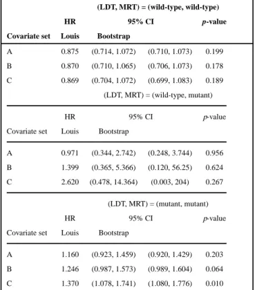
We then model the overall survival using the proposed pattern mixture model. Because we did not observe the combination of KRAS mutant per LDT and KRAS wild-type per MRT, we consider a modified version of pattern mixture model with three possible patterns. We consider three pattern mixture models with covariate sets A, B, or C, as defined in Section 5.1. The estimated hazard ratios for panitumumab plus FOLFOX in subjects with different combinations of test statuses under pattern mixture models are shown in Table IV. The confidence intervals for hazard ratios are estimated using both Louis’ formula and the bootstrap method [11], which is also a commonly used method in variance estimation. In all the models we considered, the treatments perform differently for subjects with different test statuses: panitumumab plus FOLFOX works better for subjects with test status (LDT, MRT) = (wild-type, wild-type), while FOLFOX alone is better for subjects with test statuses (LDT, MRT) = (mutant, mutant). For subjects with test statuses (LDT, MRT) = (wild-type, mutant), the estimated hazard ratios have wide confidence intervals, because of the small number of subjects in this category. Compared with the bootstrap confidence interval, the confidence intervals formulated using Louis’ formula are narrower and thus give more precision.
We plot the estimated survival curves for different treatment groups under model with covariate set C in Figure 1. Specifically, we plot different subgroups of subjects with
A
uthor Man
uscr
ipt
A
uthor Man
uscr
ipt
A
uthor Man
uscr
ipt
A
uthor Man
uscr
different statuses per LRT or MRT separately, where the dotted curves indicate the bootstrap 95% confidence interval. We estimated the difference in test-specific restricted mean survival time for different treatment groups, and the results are shown in Table V. The treatment differences in the restricted mean survival time are positive in wild-type by LDT and MRT, and are negative in mutant by LDT and MRT, indicating that panitumumab plus FOLFOX is beneficial for the wild-type subjects, and FOLFOX alone is preferred for the mutant subjects.
We assess the proportional hazards assumption for the pattern mixture model through the proportional hazards tests based on Schoenfeld residuals [12]. Prior to the proportional hazards tests, we impute the missing test statuses by the statuses with the largest estimated probability pkl(X). The global tests for proportional hazards assumption have p-values 0.290,
0.255, and 0.656 for pattern mixture models with covariate set A, B, and C, respectively, indicating that the proportional hazards assumptions for the pattern mixture models are adequate.
6. Discussion
In this paper, we consider a pattern mixture model to perform clinical validation of MRT when the ascertainment rate for biomarker status per MRT is relatively low. Even though the most common scenario is to handle two tests (MRT and LDT), we establish a general framework accommodating arbitrary number of tests. We use the EM algorithm to address the issue of missing data. We illustrate the method in a clinical study, compared with the proportional hazards model based on complete cases and bootstrapping with imputation. The results are similar in terms of the point estimates and p-values.
Compared with the bootstrapping with imputation method developed by Denne et al. [3], where subjects with non-missing LDT statuses are included, our method utilize the information from all the subjects in the clinical study. The missing LDT statuses are also regarded as missing values, and are taken into account in the EM algorithm. This avoids the potential issues when the subjects with non-missing LDT statuses are not representative of the whole study population. The inclusion of those subjects gives unbiased results when the LDT statuses is missing at random, and it gives statistically more efficient results.
The pattern mixture proportional hazards assumption may not be valid in practice. However, we showed in the simulation studies that even when the model is misspecified, the estimated treatment effects are close to the true values, and the confidence intervals for the treatment effects have coverage probabilities close to the nominal values. The proposed method thus gives valid approximation for the treatment effects.
In addition to the test-specific hazard ratios, we obtain the hazard ratios for subjects with combinations of test statuses using our method. The combination of test statuses intuitively gives more accurate characteristics on the biomarker status, and may also be preferable in identifying the population for the targeted therapies.
A
uthor Man
uscr
ipt
A
uthor Man
uscr
ipt
A
uthor Man
uscr
ipt
A
uthor Man
uscr
Supplementary Material
Refer to Web version on PubMed Central for supplementary material.
References
1. US Food and Drug Administration. Guidance for industry and Food and Drug Administration staff: in vitro companion diagnostic devices. 2014. Available at https://www.fda.gov/downloads/ medicaldevices/deviceregulationandguidance/guidancedocuments/ucm262327.pdf[Accessed on 25 April 2017]
2. Woodcock J. Assessing the clinical utility of diagnostics used in drug therapy. Clinical Pharmacology and Therapeutics. 2010; 88(6):765–773. [PubMed: 20981005]
3. Denne JS, Pennello G, Zhao L, Chang SC, Althouse S. Identifying a subpopulation for a tailored therapy: bridging clinical efficacy from a laboratory-developed assay to a validated in vitro diagnostic test kit. Statistics in Biopharmaceutical Research. 2014; 6(1):78–88.
4. Ibrahim JG. Incomplete data in generalized linear models. Journal of the American Statistical Association. 1990; 85(411):765–769.
5. Douillard JY, Siena S, Cassidy J, Tabernero J, Burkes R, Barugel M, Humblet Y, Bodoky G, Cunningham D, Jassem J, Rivera F, Kocakova I, Ruff P, Blasinska-Morawiec M, Smakal M, Canon JL, Rother M, Oliner KS, Wolf M, Gansert J. Randomized, phase III trial of panitumumab with infusional fluorouracil, leucovorin, and oxaliplatin (FOLFOX4) versus FOLFOX4 alone as first-line treatment in patients with previously untreated metastatic colorectal cancer: the PRIME study. Journal of Clinical Oncology. 2010; 28(31):4697–4705. [PubMed: 20921465]
6. QIAGEN Manchester Ltd. TherascreenⓇ KRAS RGQ PCR Kit. 2012. Available at https:// www.qiagen.com/us/shop/detection-solutions/personalized-healthcare/therascreen-kras-rgq-pcr-kit-us/#productdetails[Accessed on April 2017]
7. Kaplan EL, Meier P. Nonparametric estimation from incomplete observations. Journal of the American Statistical Association. 1958; 53(282):457–481.
8. Louis TA. Finding the observed information matrix when using the em algorithm. Journal of the Royal Statistical Society Series B (Statistical Methodology). 1982; 44(2):226–233.
9. Ibrahim JG, Chen MH, Lipstiz SR. Monte Carlo EM for missing covariates in parametric regression models. Biometrics. 1999; 55(2):591–596. [PubMed: 11318219]
10. Gail M, Simon R. Testing for qualitative interactions between treatment effects and patient subsets. Biometrics. 1985; 41(22):361–372. [PubMed: 4027319]
11. Davison, AC., Hinkley, DV. Bootstrap Methods and Their Application. Cambridge University Press; London: 1997.
12. Grambsch PM, Therneau TM. Proportional hazards tests and diagnostics based on weighted residuals. Biometrika. 1994; 81(3):515–526.
A
uthor Man
uscr
ipt
A
uthor Man
uscr
ipt
A
uthor Man
uscr
ipt
A
uthor Man
uscr
Figure 1.
Estimated survival curves of different treatment groups for subjects with different test statuses. [Colour figure can be viewed at wileyonlinelibrary.com]
A
uthor Man
uscr
ipt
A
uthor Man
uscr
ipt
A
uthor Man
uscr
ipt
A
uthor Man
uscr
A
uthor Man
uscr
ipt
A
uthor Man
uscr
ipt
A
uthor Man
uscr
ipt
A
uthor Man
uscr
T ab le ISummary statistics for simulation results.
n = 250 n = 500 n = 1000 P arameter Bias SE SEE CP Bias SE SEE CP Bias SE SEE CP η00 0.041 0.496 0.452 0.934 0.017 0.315 0.301 0.937 0.008 0.211 0.207 0.947 0.035 0.500 0.452 0.931 0.016 0.313 0.301 0.941 0.012 0.212 0.207 0.947 0.038 0.880 0.798 0.930 0.020 0.551 0.526 0.941 0.016 0.365 0.360 0.947 η01 −0.014 0.749 0.678 0.931 −0.001 0.475 0.456 0.943 0.001 0.320 0.315 0.947 0.030 0.264 0.252 0.940 0.013 0.180 0.175 0.941 0.007 0.123 0.122 0.948 0.024 0.277 0.258 0.932 0.012 0.182 0.178 0.948 0.005 0.126 0.125 0.950 0.003 0.467 0.438 0.935 −0.001 0.309 0.302 0.949 0.002 0.215 0.211 0.947 η10 0.027 0.832 0.753 0.933 0.015 0.527 0.502 0.938 0.014 0.352 0.346 0.947 −0.039 0.426 0.394 0.934 −0.017 0.277 0.266 0.946 −0.011 0.188 0.184 0.947 −0.009 0.428 0.397 0.934 −0.004 0.278 0.268 0.943 −0.002 0.190 0.186 0.945 0.047 0.757 0.690 0.936 0.021 0.480 0.463 0.946 0.007 0.324 0.319 0.949 η11 0.024 0.829 0.756 0.933 0.014 0.521 0.504 0.941 0.013 0.347 0.347 0.952 −0.030 0.434 0.397 0.934 −0.020 0.278 0.268 0.941 −0.011 0.187 0.186 0.951 0.041 0.426 0.397 0.936 0.020 0.276 0.268 0.942 0.008 0.190 0.185 0.945 −0.010 0.754 0.696 0.933 0.002 0.485 0.467 0.942 −0.003 0.322 0.322 0.952 θ01 0.023 0.499 0.482 0.950 0.007 0.338 0.335 0.949 0.004 0.234 0.235 0.953 0.005 0.440 0.432 0.952 0.002 0.306 0.300 0.948 0.003 0.212 0.211 0.952 0.018 0.779 0.750 0.948 0.015 0.527 0.521 0.951 0.004 0.366 0.366 0.951 θ10 0.005 0.550 0.532 0.951 −0.002 0.375 0.369 0.951 −0.002 0.259 0.259 0.956 0.011 0.494 0.483 0.951 0.002 0.342 0.336 0.950 0.008 0.237 0.235 0.947 0.006 0.863 0.836 0.946 0.012 0.587 0.580 0.949 0.002 0.409 0.407 0.949 θ11 0.003 0.545 0.531 0.950 −0.002 0.379 0.369 0.949 0.001 0.256 0.258 0.953 −0.008 0.492 0.483 0.951 0.000 0.341 0.335 0.948 −0.001 0.233 0.235 0.954 0.026 0.856 0.836 0.951 0.015 0.600 0.580 0.945 0.007 0.408 0.407 0.950
Note: Bias, SE, SEE, and CP denote the mean bias, standard de
viation, mean standard error estimates, and co
v
erage probability of 95% conf
idence interv
als, respecti
v
ely
A
uthor Man
uscr
ipt
A
uthor Man
uscr
ipt
A
uthor Man
uscr
ipt
A
uthor Man
uscr
ipt
T ab le IISummary statistics for simulation results in misspecif
ied model. n = 250 n = 500 n = 1000 P arameter Bias SE SEE CP Bias SE SEE CP Bias SE SEE CP η00 0.109 0.553 0.455 0.902 0.075 0.347 0.300 0.905 0.061 0.231 0.206 0.909 0.103 0.560 0.455 0.893 0.076 0.345 0.301 0.907 0.068 0.232 0.206 0.907 0.102 0.983 0.803 0.900 0.078 0.608 0.525 0.912 0.073 0.400 0.357 0.917 η01 0.594 0.791 0.669 0.826 0.593 0.487 0.447 0.726 0.590 0.323 0.308 0.518 −0.012 0.233 0.236 0.953 −0.031 0.155 0.164 0.958 −0.040 0.107 0.115 0.954 −0.018 0.240 0.240 0.949 −0.034 0.158 0.166 0.957 −0.042 0.108 0.116 0.954 0.002 0.407 0.410 0.952 −0.001 0.268 0.284 0.966 0.003 0.186 0.198 0.963 η10 0.923 0.898 0.732 0.717 0.872 0.563 0.486 0.559 0.848 0.375 0.334 0.302 −0.098 0.436 0.361 0.893 −0.077 0.282 0.244 0.903 −0.070 0.192 0.169 0.894 −0.017 0.435 0.364 0.904 −0.009 0.284 0.246 0.912 −0.005 0.194 0.170 0.915 0.108 0.768 0.633 0.897 0.078 0.491 0.425 0.910 0.070 0.330 0.293 0.913 η11 1.137 0.848 0.730 0.629 1.086 0.529 0.485 0.392 1.064 0.352 0.333 0.115 −0.017 0.384 0.354 0.932 −0.008 0.247 0.240 0.944 0.000 0.167 0.166 0.951 0.030 0.378 0.356 0.934 0.013 0.250 0.241 0.942 0.004 0.169 0.167 0.948 −0.014 0.669 0.622 0.935 −0.003 0.434 0.419 0.944 −0.009 0.287 0.290 0.953 θ01 0.028 0.497 0.480 0.950 0.009 0.337 0.334 0.949 0.005 0.233 0.235 0.952 0.003 0.441 0.431 0.952 0.001 0.306 0.300 0.948 0.003 0.212 0.211 0.951 0.015 0.778 0.748 0.947 0.013 0.527 0.520 0.951 0.004 0.366 0.365 0.950 θ10 0.007 0.549 0.530 0.949 −0.001 0.374 0.368 0.952 −0.002 0.258 0.258 0.955 0.010 0.494 0.482 0.950 0.002 0.341 0.335 0.949 0.008 0.237 0.235 0.948 0.005 0.862 0.834 0.947 0.012 0.586 0.579 0.949 0.002 0.408 0.406 0.949 θ11 0.008 0.543 0.529 0.950 0.001 0.377 0.367 0.948 0.002 0.255 0.257 0.953 −0.008 0.492 0.482 0.952 0.000 0.340 0.335 0.947 −0.001 0.233 0.235 0.953 0.022 0.854 0.833 0.950 0.012 0.598 0.579 0.946 0.005 0.407 0.406 0.950
Note: Bias, SE, SEE, and CP denote the mean bias, standard de
viation, mean standard error estimates, and co
v
erage probability of 95% conf
idence interv
als, respecti
v
ely
A
uthor Man
uscr
ipt
A
uthor Man
uscr
ipt
A
uthor Man
uscr
ipt
A
uthor Man
uscr
T ab le III T est-specific hazard ratio estimates from complete cases.
W
ild-type by LDT
Mutant by LDT
q-int test Co v ariate set HR 95% CI p -v alue HR 95% CI p -v alue p -v alue A 0.859 (0.701, 1.053) 0.144 1.150 (0.908, 1.455) 0.246 0.067 B 0.858 (0.700, 1.052) 0.142 1.256 (0.988, 1.595) 0.062 0.018 C 0.860 (0.699, 1.059) 0.157 1.368 (1.069, 1.751) 0.013 0.005 W
ild-type by MR
T
Mutant by MR
T q-int test Co v ariate set HR 95% CI p -v alue HR 95% CI p -v alue p -v alue A 0.865 (0.693, 1.079) 0.197 1.139 (0.906, 1.433) 0.266 0.090 B 0.870 (0.697, 1.086) 0.219 1.236 (0.980, 1.559) 0.074 0.032 C 0.913 (0.727, 1.146) 0.433 1.337 (1.052, 1.698) 0.018 0.024
Note: HR, 95% CI, and
p
-v
alue denote the estimate, 95% conf
idence interv
al, and
p
-v
alue for the test-specif
ic hazard ratio for panitumumab plus FOLFO
X compared with FOLFO
X alone, respecti
v ely . Q-int test p -v
alue denotes the
p
-v
alue for quantitati
v
e interaction test. LDT
, laboratory-de
v
eloped test; MR
T
, mark
A
uthor Man
uscr
ipt
A
uthor Man
uscr
ipt
A
uthor Man
uscr
ipt
A
uthor Man
uscr
ipt
Table IV
Hazard ratio estimates for combined tests from the pattern mixture model.
(LDT, MRT) = (wild-type, wild-type)
HR 95% CI p-value
Covariate set Louis Bootstrap
A 0.875 (0.714, 1.072) (0.710, 1.073) 0.199
B 0.870 (0.710, 1.065) (0.706, 1.073) 0.178
C 0.869 (0.704, 1.072) (0.699, 1.083) 0.189
(LDT, MRT) = (wild-type, mutant)
HR 95% CI p-value
Covariate set Louis Bootstrap
A 0.971 (0.344, 2.742) (0.248, 3.744) 0.956
B 1.399 (0.365, 5.366) (0.120, 56.25) 0.624
C 2.620 (0.478, 14.364) (0.003, 204) 0.267
(LDT, MRT) = (mutant, mutant)
HR 95% CI p-value
Covariate set Louis Bootstrap
A 1.160 (0.923, 1.459) (0.920, 1.429) 0.203
B 1.246 (0.987, 1.573) (0.989, 1.604) 0.064
C 1.370 (1.078, 1.741) (1.080, 1.776) 0.010
A
uthor Man
uscr
ipt
A
uthor Man
uscr
ipt
A
uthor Man
uscr
ipt
A
uthor Man
uscr
T
ab
le V
Estimated restricted mean survi
v
al time dif
ference from pattern mixture model.
W
ild-type by LDT
Mutant by LDT
Co
v
ariate set
Estimate
95% CI
p
-v
alue
Estimate
95% CI
p
-v
alue
A
45.6
(−24.4, 115.6)
0.201
−52.2
(−132.4, 28.1)
0.203
B
44.5
(−24.1, 113.1)
0.203
−70.2
(−147.1, 6.7)
0.074
C
49.8
(−18.6, 118.1)
0.153
−91.6
(−167.6, −15.5)
0.018
W
ild-type by MR
T
Mutant by MR
T
Co
v
ariate set
Estimate
95% CI
p
-v
alue
Estimate
95% CI
p
-v
alue
A
47.0
(−24.6, 118.6)
0.198
−48.7
(−127.0, 29.6)
0.223
B
49.3
(−21.5, 120.0)
0.172
−70.1
(−144.2, 4.0)
0.064
C
58.9
(−11.8, 129.6)
0.103
−94.8
(−167.5, −22.1)
0.011
Note: HR, 95% CI, and
p
-v
alue denote the estimate, bootstrap 95% conf
idence interv
al, and
p
-v
alue for the test-specif
ic hazard ratio for panitumumab plus FOLFO
X compared with FOLFO
X alone,
respecti
v
ely
. Q-int test
p
-v
alue denotes the
p
-v
alue for quantitati
v
e interaction test. LDT
, laboratory-de
v
eloped test; MR
T
, mark