Available online at www.cuijca.com
International Journal of Computational Analysis Vol (2), No. (2), pp. 16-21
* Corresponding author: E-mail address: [email protected]
Effect of roots and runners in Strawberry Algorithm for optimization Problems
Nudrat Aamir
1,*, Mehwish Mushtaq
1, Rosmeena Riaz
21Shaheed Benazir Bhutto Women University Peshawar, Pakistan 2Independent Researcher
Keywords:
Strawberry Algorithm Effect of Roots and Runners Optimization problem
ABSTRACT
It is usually difficult for humans to solve a real world problem. Although for millions of years nature has its own ways to look into these problems and solve them. Hence, now a days when man made methods do not work in these situations, they turn to Nature for problem solution. Therefore, the so called Nature inspired algorithms/ Heuristics are developing rapidly. Generally it is difficult to find the optimum solution of the problem by using Heuristic methods. On the other hand these methods are good in approximating the solution in justifiable time. One of such algorithm is known as Strawberry Algorithm (SBA). Here, we propose to investigate the effect of roots and runners in SBA
.
1. Introduction
Nature has played an important role for development of new optimization algorithms for the solution of complex engineering problems. Rechenberg was among first researchers who tried to develop a cybernetic (the science of communications and automatic control systems in both machines and living things) solution to a practical problem. However, Holland developed the genetic algorithm (GA), one of first of its kind, used for the solution of complicated problems. Till date a variety of nature inspired algorithms are available such as the GA, Particle Swarm Optimization (PSO) [1], [2], Ant Colony Optimization (ACO) [3], [4], Artificial Bee Colony (ABC) algorithm [5], [6], Simulated Annealing (SA) [7], [8], Firefly Algorithm (FA) [9], Bacterial Foraging Optimization (BFO) [10], Artificial Immune System (AIS) [11], [12], shuffled frog-leaping algorithm [13], Differential Evolution (DE) [14], [15], and Imperialist Competitive Algorithm (ICA) [16], have attracted more attentions. Enormous best approximation solutions in complicated engineering problems have been found through these techniques [17], [18], [19]. Though, these algorithms are different in nature but they have some similarities, usually in the form of application of random variable, how they deal with uncertain and non differentiable functions, use of more than one computational agent for finding the domain of problem except SA where only one agent is used, use of function values rather than using its derivatives. All these nature inspired algorithms uses the behaviour of a certain living thing or its colony or some physical activity by performing some type of optimization. In order to model such algorithm random variables are used for iteration, also in these procedures the algorithm remembers the good solution of previous steps and uses it as finest agent of the colony which will have more chances of survival and reproduction.
All above mentioned algorithms have some advantages and disadvantages, none of the above algorithm can be described as best due to the fact that every algorithm behaves well in certain conditions. As one of the main reason for an algorithm to be considered as best is the turning parameters, fewer the turning parameters better the algorithm. Keeping in mind the above mentioned fact, the intelligent water drops (IWD) algorithm is not considered as good algorithm as it uses too many tuning parameters without giving any general procedure. PSO is fast but some time when it is trapped in local minimum it’s hard for algorithm to escape it. SA has disadvantage of sensitivity to initial guess and have low chances of finding global solution Though GA has advantage over PSO that its solution is always within the region defined by boundaries defined by variables, on the other hand GA has disadvantage of being slow and having restricted accuracy due to coding [20], [21]. Hence it can be concluded from above discussion that any algorithm which uses less tuning parameters in trial and tuning process is more effective, have faster convergence rate and more possibility of escaping from local optimum. On the other hand
effectiveness of these algorithms depends on problem considered, as one algorithm may behave well in one type of problem and may behave worse in other problems. Strawberry algorithm (SBA) is also one such type of algorithm, inspired from strawberry plant, used for solution of multi variable problems [22]. The main difference between SBA and other natured inspired algorithms [23] is that here the number of computational agents (an important factor in each algorithm) differ from start till end. In this algorithm half of the weak agents are discarded and good agents are duplicated at each iteration [22]. Few other advantages of SBA are that the agents comprise of both large and small movements throughout hence making it possible to find the local and global optima at the same time. Another main difference among SBA and other algorithms is that in SBA the agents does not affect other agents. Therefore, to find the local and global search, at each iteration runners and roots both are developed through this algorithm. Another of this type of algorithm is known as seed based algorithm [24], where queuing process result in seed based search algorithm. Here researchers have used the idea of SBA but instead of using runners and roots they have considered strawberry seeds for propagation.
1.1 Strawberry Algorithm
Humans and animals have superiority over plants in many ways, as they have brain and muscles which help them to bear the ecological changes around them and help them to migrate to places with better environmental conditions. The migrants, both humans and animals, during war time and natural disasters, is one of the best example of one of their edge over plants. On the other hand plants (in most cases) cannot propagate freely, due to the fact that they are attached to the soil. However, propagation is possible in some types of pastures and plants (like strawberry) through, both, roots and runners. The roots and runners are produced by the parent plant (also known as mother plant), one side of the runner is attached to mother plant whereas the other side is free to move. The free side then produces another plant when landed to fertile land, otherwise, it dies. This new plant, produced by runner of mother plant, is also known as daughter plant. The runner has few unwarranted roots which grows when landed to fertile land. When the daughter plant, produced by the runner, has sufficient roots it can be separated by mother plant and can itself now behave like mother plant. It has been observed that the mother plant usually dies earlier than the daughter plant unless daughter plant lands on the land with bad conditions.
It has been observed by F. Merrikh-Bayat [22] that strawberry plants (or any other plants with runners) are very good examples of optimization, as both global and local search is being performed by these type of plants. Furthermore, it was also pointed out that development of runners and roots is purely random, but it does effect mother plant if runner or root hairs finds a fertile land with lot of water resources which basically helps the daughter plant to grow more roots and runners. F. Merrikh-Bayat had modelled the behaviour of these plants to find the optimization algorithm. The algorithm was modelled for global and local search by considering three facts:
1. Roots and its hairs are developed by mother strawberry plant randomly (to check the local search for fertile land). 2. Runners (generated randomly) propagate each strawberry plant (to find the global search for resources).
3. Survival of each strawberry daughter plant depends on its access, if landed to fertile area it will grow faster and will die if lands on poor resources. Hence, the SBA is developed by first generating few points (each of them considered as mother plant) in the domain of problem, called computational agents. Furthermore, single root and single runner (daughter plant) is generated by mother plant in each iteration, root will be in very near location and runner in farther locality. Hence, the computational agents contains the roots and runners who’s movement in domain of the problem is considered as small and large steps. Then the roots and runners in computational agents evaluates the objective function, among the points considered half are selected on basis of higher fitness level produced by the agents (points). In algorithm this procedure is repeated unless it satisfies the termination criteria given in algorithm.
1.2 Genetic Algorithm
Many researchers have worked on understanding the link between machine learning and nature’s system and finding the way how machine learning can perform better while borrowing from nature [25], [26]. One of such algorithm which inspired the researchers is Genetic Algorithm (GA). Charles Darwin’s theory of natural evaluation inspired researchers to develop the search investigation known as GA. In this algorithm natures process of selection is used to select the individuals (which have best fitness among them self) for reproduction to generate the descendants (off springs) of future generation.
In GA consists of five phases: 1. Early population (or initialization) 2. Fitness Value (or function) 3. Selection
4. Crossover 5. Mutation
In GA, basically iterative process is used in order to find the solution of considered optimization problem [27]. In this process, a set of individuals is considered known as Population set, here it is important to note that each individual is solution to the problem considered. Furthermore, each individual is categorized by number of factors called Genes. These genes are then connected to strings to formulate a Chromosome (known as solution to problem). These randomly chosen individuals are used at each iteration and are known as generation. In this process each individual has to pass through the fitness process (or function), which determines how fit each individual is when compared to other individual. This process provides a fitness point to every individual.
Hence, selection of individual for future generation depends on the point values given by these fitness functions. In third phase, selection process, the individuals (parents) with best fitness scores are selected authorizing them to pass on their genes to future generation. The crossover phase is the most important one, in this phase randomly a crossover point is chosen for every pair of parents. The parents exchanges the genes, unless the crossover point is reached, and produces the off springs. These newly produced off springs becomes part of the population. Among these new offspring some are subjected to the next phase, known as mutation, in this process some points or bits can be turned over in bit string. This process is mainly used to avoid the reproduction of same off-springs and avoid the convergence before time. This algorithm stops when termination criteria is fulfilled, means, the population does not produces next generation, which is different from previous one. The set obtained after termination criteria is satisfied is called the solution set to our problem.
2. Mathematical Description of Strawberry Algorithm
The Strawberry algorithm tries to finds the solution of unconstrained optimization problem defined as: min g(y), yl ≤ y ≤ yu ,
where
g : Rn → R,
is an n dimensional objective function (also known as cost function) to be minimized, y ∈ Rn is the solution vector and y
l,yu ∈ Rn are the upper and lower
limits of the variable. The SBA works on following points: for the solution of above problem in the domain of the above problem N points are considered, each known as mother plant. Then in next step, two arbitrary points (one very near to mother plant and other far away from it) are generated by each of these mother plants at each iteration, behaving like roots and runners (daughter plant) in case of strawberry plant. The points which are faraway, basically avoids the trapping in local minimum and hence results in helping the algorithm to find the global minimum. Where at j−th iteration the k−th mother plant is represented by the points yk(j)∈ Rn where k = 1,...,N, and Ylocat(j) represents the matrix which consists of runners and roots generated by N mother plants.
This matrix can be calculated by
Ylocat(j) = [Yroot(j)Yrun(j)] = [Y (j)Y (j)] + [prootr1prunr2], 1.1
Where
Y (j) = [y1(j)y2(j)....yN(j)], Yloct(j) = [y1,locat(j)y2,locat(j)...y2N,locat(j)], and Yroot(j),Yrun(j) ∈ Rn∗N defines the location of roots and runners in following manner:
Yroot(j) = [y1,root(j)y2,root(j)...yN,root(j)], 1.2
Yrun(j) = [y1,run(j)y2,run(j)...yN,run(j)], 1.3
where independent arbitrary values with uniform distribution is represented by matrices r1,r2 ∈ Rn∗N. On the other hand distance of roots and runners from
their respective mother plant is represented by scalars p1, p2, such that prun >> proot.
As mentioned above, each mother plant generates two points hence Ylocat(j) (which contain the expected solution) has 2N columns and Y (j) only N columns.
In order to select the N columns out of 2N columns calculated through Yloct(j), authors have used roulette wheel (or any such scheme can be used) depending
on which vector have higher chances for selection as a mother plant for the future. It has been observed by the researchers [22] that elite and random selection combined together produces the best result for selection of these N points Hence, in SBA, elite selection chooses half of the best N future mother plant and roulette wheel selects the other half from 2N columns of Yloct(j). However, in order to select the other half best N future mother plants among the 2N columns,
first the fitness of kth column of Yloct(j) is calculated in a similar method as in ABC, by using following equation,
, ,
,
, ,
1
( ) 0, 1, 2,... ( )
( )
( ) ( ) 0
k loct k loct
k loct
k loct k loct
g y j k N
a g y j
fit y j
a g y j g y j
1.4
where the function to be minimized is represented by g(x) and parameter a ≥ 0 (in SBA it is considered as 0). Furthermore, once the fitness value is calculated possibility of randomly choosing the kth column c
k is calculated by following formula:
ck = fracfit(yk,loct(j)) ∑𝑁𝑘=1𝑓𝑖𝑡(yk,loct(j)). 1.5
Hence, the selected values through above mentioned process will be considered as mother plants for next iteration.
2.1 The pseudo code of Strawberry Algorithm
1: Procedure Initialize proot,prun and N. 2: Set j := 0
3: From domain of the problem choose randomly the values of N mother plants, hence, each value resulting in as a column of Y (0). 4: WHILE (the termination criteria is not satisfied).
5: Duplication: From each mother plant calculate the daughter plant and root from eq(2) and each calculated value is considered as a column entry for Yloct(j).
6: Elimination: From 2.1.5 determine the root and runner fitness then selecting the N future mother plants from 2N values. These values will be considered as columns of Y (j + 1).
8: EndWhile
3. Test Functions
Any new approach for the solution of optimization problem have to be tested for validation through different test functions already present in literature, known as benchmark problems or functions. Hence the proposed idea is tested on Rastrign function (4 variables), Griewank function (2 variables) and Schwefel function (2 and 4 variables), which are considered as badly behaved functions [31] [32].
3.1 Rastrigin’s Function
The Rastrigin’s Function have few minima and its shape is flatter than some other testing functions, such as Ackley’s function which some time complicates the conver gence towards minima at xi = 0. The function is defined as:
𝑓(𝑥) = 10𝑑 + ∑ [𝑥2− 10 cos (2𝜋𝑥
𝑖)] 𝑑
𝑖=1 ,
where d is the dimension. It’s global minimum is f(x∗) = 0 at x∗ = (0,0,...,0). Dimension 4 will be tested for the proposed algorithm.
3.2 Griewank’s Function
To test the convergence of optimization algorithms Griewank function is widely used, and is defined by,
𝑓(𝑥1, 𝑥2, 𝑥3, … … 𝑥𝑛) = 1 +
1
4000∑ 𝑥
2 𝑛
𝑖=1
− ∏ cos [𝑥𝑖
√𝑖]
𝑛
𝑖=1
for xi ∈ [−600,600] with global minima at x = 0. Here dimension 2 will be taken in considration.
3.3 Schwefel’s Function
The Schwefel function is one of the complex functions and behaves badly in different algorithms due to the fact that it has many local minima.
𝑓(𝑥) = 418.9829 𝑑 − ∑ 𝑥𝑖sin (√|𝑥𝑖|)
𝑑
𝑖=1
It has global minimum f(x∗) = 0 at x∗ = (420.9687,...,420.9687). In this paper the function will be tested for two and four variable.
4. Numerical Results
The main purpose of this section is to report and analyze the numerical results of the idea proposed in this paper. Hence, to compare the numerical performance of Strawberry Algorithm by compairing the effect of roots and runners on badly behaved functions. The numerical performance of SBA with number of runners and roots are 500 and 20 / 300 and 20 will be compared and analyzed with standard SBA.
In order to compare the above mentioned methods following parameters are taken in account for testing: • Mother plants; N= 50, N ∈ E (even number).
• m = 20; number of variables.
• (ul,uh) = (−600,600) upper and lower bound of variables. • (drunner,droot) = (400,10) (length of runners and roots).
The numerical results for these functions are reported as:
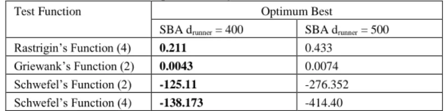
4.1 Comparison of SBA with drunner = 400 and 500 droot = 20
Here our focus is on comparison of SBA in case if different roots and runners are considered, for comparison here the number of runners selected are drunner
= 400 & 500 and droot = 20. The numerical results in Table 1 show that the performance is comparable in case of Rastrigin and Griewank Function. Otherwise,
if drunner = 400 Schwefel (with dimension 2 and 4) is performing much better.
Table 2: Comparative Analysis of drunner = 400 & 500
Test Function Optimum Best
SBA drunner = 400 SBA drunner = 500
Rastrigin’s Function (4) 0.211 0.433
Griewank’s Function (2) 0.0043 0.0074
Schwefel’s Function (2) -125.11 -276.352
4.2 Comparison of SBA with drunner = 400 and 300 droot = 20
In this subsection we focus on comparison of SBA in case if different roots and runners, for comparison here the number of runners selected are drunner =
400 & 300 and droot = 20. It is evident from Table 2 that SBA is again winning when drunner = 400 in case of Rastrigin and Schwefel (dimension 2 and 4)
functions, where on the other hand it is comparable in case of Griewank Function when drunner = 300
Table 1: Comparative Analysis of drunner = 400 & 300
Test Function Optimum Best
SBA drunner = 400 SBA drunner = 500
Rastrigin’s Function (4) 0.211 18.147
Griewank’s Function (2) 0.0043 0.0036
Schwefel’s Function (2) -125.11 -276.352
Schwefel’s Function (4) -138.173 -414.40
5. Conclusion
In plants or seeds, location search can be considered as search process in optimization algorithms. In this work , strawberry algorithm is considered and is numerically experimented. Furthermore, it was highlighted that roots and runners can be considered as local and global search. Therefore, in this work we considered different values of roots and runners and observed the effect of them on finding the search direction. It has been observed that,
Change in value of runner does not give any promising results.
On the other hand it has been observed that change in the value of runners does effect the search differently for different situations. Hence, it has been observed by experimental results that SBA can have different values of runners depending on problem under consideration. Furthermore, numerical results reveal that, generally, any number of roots contribute good result if considered with d_runner = 400.
5.1 Future Plan
This idea will further be explored with new scheme where the parameters in SBA be taken with different values.
REFERENCES
[1] Y. Shi et al (2001)., “Particle swarm optimization: developments, applications and resources,” in CE. [2] R. Eberhart and J. Kennedy (1995), “A new optimizer using particle swarm theory,” in MHS’95.
[3] M. Dorigo and M. Birattari (2011), “Ant colony optimization,” in Encyclopedia of Machine Learning, pp. 36–39, Springer.
[4] M. Dorigo, M. Birattari, and T. Stu¨tzle (2006), “Ant colony optimization-artificial ants as a computational intelligence technique,” IEEE Computational Intelligence Magazine, vol. 1, no. 4, pp. 28–39.
[5] D. Karaboga and B. Basturk (2008), “On the performance of artificial bee colony (abc) algorithm,” Appl. Soft Comput, vol. 8, no. 1, pp. 687– 697.
[6] D. Karaboga and B. Basturk (2007), “A powerful and efficient algorithm for numerical function optimization: artificial bee colony (abc) algorithm,” J. Global Optim, vol. 39, no. 3, pp. 459–471.
[7] V. ˇCerny` (1985), “Thermodynamical approach to the traveling salesman problem: An efficient simulation algorithm,” J. Optim. Theory and Appl, vol. 45, no. 1, pp. 41–51.
[8] S. Kirkpatrick, C. D. Gelatt, and M. P. Vecchi (1983), “Optimization by simulated annealing,” Science, vol. 220, no. 4598, pp. 671–680. [9] X.-S. Yang (2010), “Firefly algorithm, stochastic test functions and design optimisation,” Inter. J. Bio-Inspired Comput, vol. 2, no. 2, pp. 78–
84.
[10] K. M. Passino (2002), “Biomimicry of bacterial foraging for distributed optimization and control,” IEEE Control Systems, vol. 22, no. 3, pp. 52–67.
[11] J. O. Kephart et al. (1994), “A biologically inspired immune system for computers,” in Artificial Life IV: Proceedings of the Fourth International Workshop on the Synthesis and Simulation of Living Systems, pp. 130–139.
[12] L. N. De Castro and J. Timmis (2002), Artificial immune systems: a new computational intelligence approach. Springer Science & Business Media.
[13] M. M. Eusuff and K. E. Lansey (2003), “Optimization of water distribution network design using the shuffled frog leaping algorithm,” J. Water Resources Planning and Management, vol. 129, no. 3, pp. 210–225.
[14] R. Storn and K. Price (1997), “Differential evolution–a simple and efficient heuristic for global optimization over continuous spaces,” J. Global Optim, vol. 11, no. 4,pp. 341–359.
[15] R. Mallipeddi, P. N. Suganthan, Q.-K. Pan, and M. F. Tasgetiren (2011), “Differential evolution algorithm with ensemble of parameters and mutation strategies,” Appl. Soft Comput, vol. 11, no. 2, pp. 1679–1696.
[16] E. Atashpaz-Gargari and C. Lucas (2007), “Imperialist competitive algorithm: an algorithm for optimization inspired by imperialistic competition,” in IEEE CEC2007., pp. 4661–4667, IEEE.
[17] Y. Del Valle, G. K. Venayagamoorthy, S. Mohagheghi, J.-C. Hernandez, and R. G. Harley (2008), “Particle swarm optimization: basic concepts, variants and applications in power systems,” IEEE Transactions on Evolutionary Computation, vol. 12, no. 2, pp. 171–195. [18] M. R. AlRashidi and M. E. El-Hawary (2009), “A survey of particle swarm optimization applications in electric power systems,” IEEE
Transactions on Evolutionary Computation, vol. 13, no. 4, pp. 913–918.
[19] P. J. Fleming and R. C. Purshouse (2002), “Evolutionary algorithms in control systems engineering: a survey,” Control Engineering Practice, vol. 10, no. 11, pp. 1223–1241.
[20] K. Ma, T. Yao, J. Yang, and X. Guan (2016), “Residential power scheduling for demand response in smart grid,” International Journal of Electrical Power & Energy Systems, vol. 78, pp. 320–325.
[21] A. Zafar, S. Shah, R. Khalid, S. M. Hussain, H. Rahim, and N. Javaid (2017), “A meta-heuristic home energy management system,” in 31st WAINA, pp. 244–250, IEEE.
[22] F. Merrikh-Bayat (2014), “A numerical optimization algorithm inspired by the strawberry plant,” arXiv preprint arXiv:1407.7399, 2014. [23] M. S. Asvini and T. Amudha (2016), “An efficient methodology for reservoir release optimization using plant propagation algorithm,”
Procedia Computer Science, vol. 93, pp. 1061–1069.
[24] [24] M. Sulaiman and A. Salhi (2015), “A seed-based plant propagation algorithm: the feeding station model,” The Scientific World Journal, vol. 2015.
[25] L. Davis and S. Coombs (1987), “Genetic algorithms and communication link speed design: theoretical considerations,” in Genetic algorithms and their applications: proceedings of the second International Conference on Genetic Algorithms: July 28-31, 1987 at the Massachusetts Institute of Technology, Cambridge, MA, Hills dale, NJ: L. Erlhaum Associates.
[26] D. E. Goldberg and J. H. Holland (1988), “Genetic algorithms and machine learning,” Machine learning, vol. 3, no. 2, pp. 95–99. [27] A. E. Eiben, J. E. Smith, et al. (1999), Introduction to evolutionary computing, vol. 53.Springer, 2003.
[28] C. A. C. Coello, “A comprehensive survey of evolutionary-based multiobjective optimization techniques,” Knowledge and Information systems, vol. 1, no. 3,pp. 269–308.
[29] I. Fister Jr, X.-S. Yang, I. Fister, J. Brest, and D. Fister (2013), “A brief review of nature-inspired algorithms for optimization,” arXiv preprint arXiv:1307.4186.
[30] X.-S. Yang and N.-I. M. Algorithms (2008), “Luniver press,” Beckington, UK, pp. 242–246.
[31] H. Mu¨hlenbein, M. Schomisch, and J. Born (1991), “The parallel genetic algorithm as function optimizer,” Parallel computing, vol. 17, no. 6-7, pp. 619–632.