Winter 2011
Model and Solution Approach for Multi objective-multi commodity
Capacitated Arc Routing Problem with Fuzzy Demand
Alireza Eydi1*, Leila Javazi2
1Department of Engineering, University of Kurdistan, Sanandaj, Iran [email protected]
2University of Kurdistan, Sanandaj, Iran [email protected]
ABSTRACT
The capacitated arc routing problem (CARP) is one of the most important routing problems with many applications in real world situations. In some real applications such as urban waste collection and etc., decision makers have to consider more than one objective and investigate the problem under uncertain situations where required edges have demand for more than one type of commodity. So, in this research, a new fuzzy chance constrained programming model based on credibility measure for CARP with two objectives: minimizing the number of vehicle and minimizing the total travel cost is formulated. In this model each required edge has demand for more than one type of commodity and also all demands for each commodity are supposed to be triangular fuzzy numbers. Then we develop a multi-objective genetic algorithm using the Pareto ranking technique and hybrid it with stochastic simulation to design an intelligent algorithm to solve the fuzzy chance constrained model. In order to improve the quality of final solutions, we also propose a new heuristic method to generate a good initial solution in initial population of genetic algorithm. Some data sets with fuzzy demand generated randomly are used to evaluate and investigate key characteristics of the new proposed model and solution approach.
Keywords: Multi objective capacitated arc routing problem; Fuzzy chance constrained
programming; Stochastic simulation; Genetic algorithm; Pareto ranking; Heuristic. 1. INTRODUCTION
The capacitated arc routing problem (CARP) is one of the most important routing problems in literature, and attracted interest of many researchers. It has numerous applications in real world situations such as urban waste collection (Dijkgraaf and Gradus, 2007), winter gritting (Eglese and Li, 1992), snow removing (Labelle et al., 2002), inspection of gas pipeline (Han et al., 2004), street sweeping (Tobin and Brinkmann, 2002), and electric meter reading (Dror and Stern, 1979). The CARP was first introduced by Golden and Wong (1981) and deals with connected and undirected graph G= (V, E), where “V” is the set of vertices (nodes) and “E” is the set of edges. Each edge of “E” has a definite travel cost and some edges have positive demand, called required edges (
*Corresponding Author
), which must be serviced by some vehicles with limited capacity. All vehicles are identical and located at a single depot. The aim of CARP is to design a set of vehicle tours of minimum total routing cost such that each tour starts and ends at the depot, each required edge is serviced by exactly one vehicle, and the total demand serviced by any vehicle most not exceed the vehicle’s capacity. Some instances (in small and medium size) of CARP can be solved by exact methods. But CARP is a NP-hard problem (Golden and Wong, 1981) and exact methods are not able to solve the large-scale instances in reasonable time. So, due to the computational complexity of the problem, the remarkable attempts have been done by researchers in developing heuristics and metahueristics algorithms to solve it. Among known heuristics, one can refer to Augment-Merge (Golden and Wong, 1981), Path-Scanning (Golden et al., 1983), Double Outer Scan (Wøhlk, 2005), and Ulusoy’s splitting heuristic (Ulusoy, 1985). Some of metaheuristics are also proposed such as tabu search (Hertz et al., 2000), guided local search (Beullens et al., 2003), variable neighborhood search (Hertz and Mittaz, 2001), tabu scatter search (Greistorfer, 2003), and memetic algorithms (Lacommeet al., 2004).
The multi-objective CARP (MOCARP) has received spars attention in the literature compare to the single-objective. In some real world applications, more than one objective must be taken into account. For example, a wastes collection company interest in to minimize the number of vehicles used to service the required edges, moreover minimizing the total distance cost. Minimizing the number of vehicles affects vehicle and manpower costs, while minimizing distance affects time and fuel resource. Therefore, CARP is a multi-objective problem naturally. The multi-objective CARP was first studied by Lacomme et al. (2006). While considering two objectives, minimizing the total distance cost and minimizing the makespan, they combine nondominated sorting genetic algorithm II (NSGA-II) (Deb et al., 2002), and their proposed approach in Lacomme et al. (2004) to solve the problem. Mei et al. (2009) investigated MOCARP for same objectives in Lacomme et al. (2006), and proposed a hybrid algorithm by combining the memetic algorithm with extended neighborhood search (MAENS) (Tang et al., 2009) with a decomposition-based method. Minimizing three objectives including the total distance cost, the longest route (makespan) and the number of vehicles simultaneously, were studied by Grandinettiet al. (2010), and they also provided an optimization-based heuristic procedure. Fleuryet al. (2005) proposed a memetic algorithm for the MOCARP with two objectives (minimizing total travel cost and minimizing makespan) and stochastic demands. In most of previous researches about CARP, all of the problem information including demand values, travel times, etc were assumed deterministic. But in real world situations such as urban waste collection, some of parameters are often non-deterministic and not precise enough. The non- deterministic parameters can be stated as either stochastic or fuzzy. A stochastic case occurs whenever some parameters are random and have a known distribution while fuzzy case occurs whenever some parameters are uncertain, subjective and ambiguous and do not have known distribution. Stochastic CARP was considered in few literatures but to the author’s knowledge, fuzzy CARP (FCARP) not has yet been studied. Fleury et al. (2004) considered stochastic CARP with Normal distributed demands. Their solution approach is based on hybrid genetic algorithm that is modified version of the memetic algorithm earlier studied in Lacomme et al. (2004). Stochastic CARP with Poisson distribution was studied by Christian et al. (2009). They developed an exact method for solving the problem and formulated the stochastic CARP as a Set Partitioning Problem and developed a Branch-and-Price algorithm, in which the pricing is done by dynamic programming. Also, Mei et al. (2010) investigated uncertain CARP with stochastic demands. They design robust solutions for uncertain environments.
routing problem where the required edges have a demand for different products, and multi-compartment vehicles are available to co-distribute these commodities. They developed a guided local search algorithm to solve it.
In this paper in order to handle more realistic situations, we investigate the multi-objective capacitated arc routing problem with multi- commodities in assumption that the demands are uncertain and cannot be determined specifically and are regarded as fuzzy variables. The assumed objectives are minimizing the total distance cost and minimizing the number of vehicles. We will present a fuzzy chance constrained program (fuzzy CCP) based on credibility measure and then for building efficient solution method, we will provide a multi-objective genetic algorithm (a powerful algorithm) solution using the Pareto ranking technique, and hybrid it with stochastic simulation to design an intelligent algorithm to solve the fuzzy chance constrained model. Finally, the designed model is a generic and applicable in refuse collection, snow removal, etc.
The remainder of this paper is organized as follows: In section 2, we will give an overview of multi-objective optimization search, and some basic concept on fuzzy set theory. In section 3, we will present a fuzzy CCP model to deal with the problem and develop a mathematical model of multi objective-multi commodity CARP with fuzzy demands (MOMC-CARPFD). The stochastic simulation and integrating it with genetic algorithm to design an intelligent algorithm to solve the proposed model is described in section 4. The computational results are devoted in section 5 and followed by concluding remarks and directions for future research in section 6.
2. BACKGROUND
2.1. Multi-objective optimization and Pareto ranking
A multi-objective optimization problem (MOP) is one in which two or more objectives contribute to the overall result. These objectives are conflict with each other, and optimizing a particular solution concerning a single objective can result in unacceptable results concerning the other objectives. The challenge is to find a set of solutions for them, which yield an optimization of the overall problem close at hand. Without loss of commonality, a multi-objective optimization problem can be briefly described as a minimization problem with n decision variables and objectives of the form:
, , … , , … , , , … ,
s.t.
, , … ,
, , … ,
Here is decision vector, is decision space, is objective vector, and is objective space. A decision vector is said to dominate a decision vector , if and only if:
1,2, … ,
1,2, … ,Also, the decision vector is said to be nondominated, if and only if: .
A decision vector is Pareto-optimal if there is no other decision vector that dominate . The set of all Pareto-optimal solutions is called the Pareto-optimal front. Many optimization techniques such as evolutionary algorithm (EA) have been proposed in the literature to solve MOP (Veldhuizen, 1999; Coello, 1999;Veldhuizen and Lamont, 2000). To find Pareto optimal front,
often has been used Pareto ranking technique based genetic algorithm. This technique was first proposed by Goldberg (1989), as a means of assigning equal probability of procreation to all non-dominated individuals (solutions) in the population. The method comprise of assigning rank 1 to the dominated individuals and removing them from competition, then finding a new set of non-dominated individuals, ranked 2, and so on. The individuals within rank 1 are the best in the current population. The individuals in each rank set represent solutions that are in some sense incomparable with one another. Individuals that are clearly superior to others in all dimensions of the problem are characterized by Pareto ranking. Note that the objective function itself no more qualifies as fitness function since it is vector valued and fitness has to be a scalar value. Thus, Pareto ranking scheme is combined into a genetic algorithm by replacing the chromosome fitnesses with Pareto ranks.
2.2. Fuzzy sets and credibility measure
The concept of fuzzy set was introduced by Zadeh (1965), and then it has been well developed and applied in a wide variety of real problems. Fuzzy set theory generalizes 0 and 1 membership values of a crisp set to a membership function of a fuzzy set. In order to measure a fuzzy event, possibility measure theory of fuzzy variable was suggested by Zadeh (1978). Lately, Liu (2006) developed credibility theory.
Definition: Let be a fuzzy variable with membership function
, and let and be real numbers. The possibility of a fuzzy event, characterized by , is defined byr u
sup
, (1)While the necessity of is defined as follow:
1 1
r u
sup . (2)
Then, the credibility measure is an average of the possibility measure and the necessity measure (see Liu (2006)), i.e.
(3) Clearly, the fuzzy event must hold if its credibility is 1, and fail if its credibility is 0. Credibility
measure is self-dual while possibility measure is not. However, for a measure, the self-dual property is very important. When the credibility value of a fuzzy event obtains 1, the fuzzy event will certainly happen; but when the possibility value of a fuzzy event obtains 1, the fuzzy event can fail to happen.
For example, consider with triangular fuzzy variable , , as edge demand whose membership function is given as follow:
0
From the definitions of possibility, necessity and credibility it is easy to obtain:
0
1
(5)
0
1
(6)
0 1
(7)
3. MODELING
3.1. Fuzzy CCP (FCCP) model
In fuzzy mathematical programming, an optimization problem is defined as follows:
min ,
s.t.
, , 1,2, … , (8)
Where x is the decision variable set, is the set of uncertain fuzzy parameters, is ith constraint of the model and f is the objective function. Similarly, a chance constrained optimization problem can be defined here as
min
s.t.
Pr , 0 ,
1,2, … , (9)
Where is the objective function, x is the set of decision variables, is the set of random parameters, Pr is the probability measure of the given probability space of the uncertain parameter and 0, 1 is the probability level with which each of the p constraints , 0 of the entire constraint set , 0 needs to be satisfied.
The development of the chance constrained programming in a fuzzy environment can be defined as follows:
min
s.t.
1,2, … , (10) Where are premeditated confidence levels to the respective constraints, {·} denotes the
credibility of the event in {·}. This means a point x is feasible if and only if the credibility measure of the set | , 0 is at least . (Mitra, 2009)
3.2. Assumptions and mathematical model of MOMC-CARPFD
Let , be a connected and undirected graph, where 1,2, … , is the set of nodes and
, | , , is the set of edges. Each edge is represented in two directions; positive (from i to j) and negative (from j to i) directions that so called arcs. Each edge (i,j) has a nonnegative cost or length , and a fuzzy demand represented by triangular fuzzy number
, , for each commodity 1,2, … , M . The edges with positive demand (for at least one commodity) are called the required edges or tasks, . Node 1 denotes the depot. A fleet of identical vehicles are located at the depot, also each vehicle has a dedicated compartments with limited and fixed capacity for each commodity . Each vehicle tour starts and ends at the depot, and each required edge is serviced exactly once i.e. just in one of its directions. The total vehicle load for commodity m at any time should not exceed the definite capacity . The objective of MOMC-CARPFD is to determine a set of tours of all required edges such that the following objectives linked to economic consideration are met:
Minimize the total distance cost
Minimize the total number of vehicles used to service
The capacity of vehicle k can also be represented as a triangular fuzzy number = ( , , ). Let the fuzzy number presenting demand at the rth required edge for commodity m, denoted by . After serving the first l tasks (required edges), the available capacity of the vehicle k for each commodity, will equal:
∑ (11)
Using the rules of fuzzy arithmetic proposed by Kaufmann and Gupta (1985) we can easily show that is also a triangular fuzzy number, i.e.
∑ , ∑ , ∑ , , (12)
Therefore, the credibility or chance that the next required edge demand does not superpass the remaining capacity of the vehicle is founded as following:
, , 0
0
, , 1
It is obvious that 0,1 .
The vehicle tours are designed in advance by using the proposed algorithm and the actual demand becomes known upon arrival at the edge. In ordering to formulation (13), deciding whether the vehicle services the next edge or not, depends on dispatcher preference size, denoted by . Parameter states the dispatcher’s policy toward risk. Lower values of show the dispatcher preference to use vehicle’s capacity as much as possible, consequently the number of cases in which the vehicle fails to service the next required edge due to small remaining capacity (for at least one commodity), are increased. But then if dispatcher be risk averse, he/she chooses a greater , hence the failure risk decreases; however the vehicle’s loading becomes smaller. Hence, according to the credibility value, a decision must be made as to whether to send vehicle to service the next required edge or comeback it to depot. In other words if ,then the vehicle should be dispatch to the next edge; else, it should be comeback to the depot, and dispatch other vehicle to the next edge. In this paper we assume that once the vehicle arrives at the required edge and its remaining capacity is not enough to service that edge (even for one commodity), it should makes a back trip to the depot to deplete and returns to the edge where it had failure and continues service along the rest of its planned tour. It is obvious there is additional cost (distance) due to tour failure. Let and be two decision variables that can be described as following:
1 If vehicle services arc , 0 Otherwise
1 If arc , is deadheaded by vehicle 0 Otherwise
It is supposing that there is no limitation on the number of vehicles that can be used, but to facilitate the model formulation, the maximum possible size of the fleet is symbolized by K. The actual number of vehicles will be found after solving the model that it would be equal to the number of routes.
The related fuzzy chance constrained model of MOMC-CARPFD based on credibility measure can be mathematically formulated as shown below:
min ∑ ∑ , ∑ , (14)
min (15)
s.t.
∑ 1, , (16)
∑ ∑ , , (17)
∑ | |, , (18)
∑ ∑ , , (19)
∑ ∑ 2, (20)
0, 1 , , , (22)
, , , (23)
The objective function (14) states that total routing costs and total fail cost should be minimized. The objective function (15) shows that the number of vehicles or routes should be minimized. Constraints (16) ensure that each task is served only by one vehicle. Chance constraints (17) assure that all required edges are visited within vehicle capacity for each commodity with a predefined confidence level. All required edges must be serviced. This constraint is met by (18). Constraints (19) are balance constraints. Constraints (20) assure that each vehicle tour start from and end at the depot. Sub-tours elimination, is satisfied by constraints (21), where δ , , ,
, : , and ER , : , . Constraints (22) and (23)
define the domain of the decision variables.
4. DESCRIPTION OR THE SOLUTION METHODOLOGY
Because of uncertainty extension in constraints of the proposed model, it would be difficult to solve this challenging problem in traditional ways. In this section, we design a hybrid intelligent algorithm integrating stochastic simulation and genetic algorithm (GA) to solve the above proposed fuzzy CCP model. GA has been discussed in many literatures, such as Gen and Cheng (2000). It is a stochastic search method based on the principle of survival of the fittest. Also GA is highly robust and avoids getting stuck at a local optimal solution. In this study, the technique of stochastic simulation is applied to simulate the actual value of demand of required edges for each commodity in order to compute the planned route costs and additional costs due to tour failure. Then stochastic simulation and genetic algorithm based on Pareto ranking are integrated to produce a hybrid intelligent algorithm for solving the model. In continuance we will describe the proposed solution methodology for solving the MOMC-CARPFD, and present a new heuristic for generating the initial good solution and a solution similarity measure that enables the algorithm to provide a better estimation to the full Pareto front.
4.1. Design of stochastic simulation
As mentioned before, the demands of the required edges are considered as triangular fuzzy number, and the actual demand of each edge becomes known upon arrival at it. Therefore we use a stochastic simulation algorithm for each feasible planned tour in order to simulate the actual demand of each required edge and to compute approximate additional costs ( ) due to tour failure. The stochastic simulation algorithm can be summarized as follows:
Step 1: the actual demand of each required edge for each commodity is generated by following
processes: (a) randomly generate a real number in the interval between the left and right bounds of the triangular fuzzy number representing demand of the edge, and calculate its membership by eq.(4); (b) generate a random number , 0,1 and compare with , if , then actual demand of the edge is equal to ;otherwise, if , is not accepted as the demand of edge. In this case, repeat the generating random numbers and until random number and are found that satisfy relation ; (c) check and repeat (a) and (b), and terminate the process when the actual demand quantity of all required edges for each commodity is simulated.
Step 2: Move forward the route designed by credibility measure, cumulate the amounts picked up
the actual demand.
Step 3: Repeat Step 1 and Step 2, M times.
Step 4: Calculate the average value of additional costs by M times simulation, and report it as the additional costs .
4.2. Genetic algorithm procedure
The general process of the proposed GA is introduced in figure 1, and the particular components are represented below.
Figure 1 Flowchart of the proposed GA 4.2.1. Solution representation
Like Lacomme et al. (2006), we represent a model solution as a chromosome, including ordered list of the tasks (required edges), denoted by , , … , . Figure 2 shows an example of solution representation. Thick arrows show the required edges and dotted arrows show the edges with least cost. There are two numbers beside each required edge. Those outside of the parentheses indicate the positive direction and those in the parentheses indicate the negative direction of each required edge. This solution (in figure 2) includes two routes, and each starts from and ends at the depot. In this representation each gene with index 0 represents in the chromosome a separator between two different routes. The corresponding routing plan can be achieved by connecting every two succeeding edges with the shortest path between them (i.e., finding a shortest path from the tail
Start
Initial population (new heuristic)
Pareto fitness evaluation and controlling diversity of
population
Tournament selection
Crossover (SBX)
Local search Stoppin
g criterion
No
Yes
node of the former edge to the head node of the succeeding edge), which can be obtained by Dijkstra’s algorithm (Dijkstra, 1959).
Figure 2 Illustration of solution representation 4.2.2. Initial population
Generating permutations randomly is a classical technique, but adding high-quality solutions always accelerates the convergence of the algorithm. For this mean while checking the capacity chance constraint (17), we used two classical CARP heuristic, namely Path-Scanning (Golden et al., 1983) and Ulusoy’s heuristic (Ulusoy, 1985) and a new proposed heuristic that is presented in the next subsection. The rest of the population is generated randomly. Note that the population size is kept constant overall the algorithm.
4.2.2.1. The new heuristic algorithm
In this section we present our new heuristic algorithm. By employing some features of “Double Outer Scan heuristic (DOS)” (Wøhlk, 2005), and “Ellipse Rule based Path-Scanning (RSE-ER)” (see Santos et al., 2009) with some differences, we present a new robust heuristic. Like DOS, we extend the current partial tour by its both of ends, but here, we use four new criteria, and like RSE-ER, we force the vehicle back to the depot when its load is near its capacity, but without servicing any edge between the last serviced edge and the depot. Finally, we merge the obtained tours in order to reduce the total cost. Our algorithm can be described as follows:
As mentioned before, we represent each edge in two directions; positive (from to ) and negative (from to ) directions that so called arcs. In order to facilitate, the arcs with positive direction and negative direction is denoted by and , respectively. Each arc has a tail node and a head node . Further, the opposite direction of arc is denoted by . Hence, the following features are notable:
; ; ; ; ; ;
Let ∑| | be the total demand of right boundary of triangular fuzzy number , be the number of required edges, and be a real parameter.
Step 1. Select one unserviced arc at random, and remove its inverse from unserviced arc set. This arc forms the current partial tour.
Suppose that the selected arc is in positive direction and is shown as , so let and be
0 1 2 0 5 4 3 0
(7)2
(9)4
(6)1
(8)3
(10)5
the first and last arcs of the current partial tour, respectively.
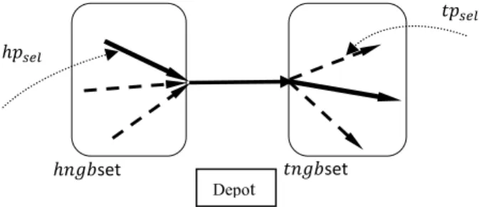
Step 2. Set as those tail-neighbor and head-neighbor required edges with such that
head-neighbor | 1 and tail-neighbor | 1 (1
denotes the depot). In order to convenience, we abbreviate tail-neighbor and head-neighbor by tngb and , respectively. Figure 3.a shows this step of the algorithm.
Step 3. Randomly choose one of following four criteria with equal probability. Then based on the result, sort the arcs in and sets.
1) Minimum distance from , to depot and Minimum distance from ,
to depot;
2) Maximum distance from , to depot and Maximum distance from ,
to depot;
3) Minimum distance from , to depot and Maximum distance from ,
to depot;
4) Maximum distance from , to depot and Minimum distance from , p
tngb to depot;
Step 4. If both set and set are not empty, choose the first arc with smaller demand to service and add it to current partial tour, and then if the remaining left boundary capacity of vehicle, , is greater than / , add another arc in another set with greater demand to current partial tour, else back to the depot (see figure 3.b). By this idea, we force the vehicle to services just those unserviced edges that are incident to the current partial tour. Consequently, more of the required edges are serviced by the vehicle in its tour. Note that when one arc is selected to service, its inverse must be deleted from unserviced arcs. If ( ) set is empty, in other words, there are no unserved edges incident to current partial tour by its head, and the remaining capacity of vehicle, , is greater than
/ , vehicle services the first arc in obtained ( ) set in step 2, otherwise it should return to the depot.
Step 5. Update set and set.
Step 6. Repeat step 2 to step 4 until vehicle load approaches its capacity or both and , becoming empty. Then connect the and to the depot by using the shortest path.
Step 7. Repeat step 1 to step 5 until all required edges to be serviced.
Step 8. Merge the constructed tours into less cost tours Subject to vehicle capacity.
Step 9. Repeat steps 1 to 8 for maximum iteration (stopping criterion) that is determine by decision maker; finally the best solution is selected.
This algorithm is same as explained before if the selected arc in step 1 be in negative direction, and just in all notations is replaced with (e.g, is replaced with ).
,
Depot
Figure 3a Illustration of forming the set and set
Figure 3b Illustration of determining the and 4.2.3. Pareto fitness evaluation and objective tradeoffs
In a multi-objective GA (MOGA), however, because of the Pareto optimality of a multi-objective optimization problem, the fitness of each chromosome is not as simple as that of a conventional GA for a single-objective problem. When solving a single-objective problem, fitness is easily assigned to an individual according to its single- objective function evaluation. In the multi-objective case, there is naturally more than one possible objective that is conflict with each other, and need to be minimized (or maximized) simultaneously. In other words a whole set of solutions is required that reflects the trade-offs between objectives. Non-dominance sorting criterion of Deb et al. (2002) is an efficient approach to assigning fitness to solutions that fulfills the current requirements. All non-dominated individuals in the current population are assigned rank one, while individuals non-dominated by one or more others are assigned rank two or higher. These ranks are then used by the GA as finesses for generating the next population. In this case the lower the front, the fitter the solution. Also here in all objectives are assumed to be minimized.
4.2.4. Controlling the diversity of population
One of the important issues in MOGA is population diversity in order to obtained solutions uniformly distributed over Pareto front. There are several methods such as crowding distance method and niching technique, for diversity preservation. The basic idea behind them is preventing the appearance of multiple solutions that are close to each other in the population. Here we use Jaccard’s similarity coefficient, which measures the similarity between two sets as ratio intersection and union of them. Garcia-Najera and Bullinaria (2009, 2011) applied this criterion for vehicle routing problem.
The Jaccard’s similarity between two sets and are measured using follow relation:
, || || (24)
set set
Depot
Subject to equation (24), the similarity is 1, if all elements in both sets are same and the similarity is 0, if both sets have no same elements. We can adapt the equation (24) in order to apply it for the MOMC-CARPFD. For this purpose we consider each solution A as a set including required edges. And so the similarity of two solutions equals the ratio between the number of two successive connections of required edges that are common to both solutions and the total number connections used by them. Let 1, if arc (i,j) is serviced by any vehicle in solution A, and 0 otherwise. Arcs (i,j) and (j,i) are considered to be different, even if their cost is the same. So the similarity between solutions A and B is
, ∑, , . . .
∑ . ∑ . ∑ . . . (25)
Suppose P is the population of solutions, D is the population size; the similarity of solution with the rest of the GA population will be given by the average similarity of A with every other solution , that is
∑ \ ,
(26) Thus the population diversity is given by equation (27):
1 ∑ (27)
4.2.5. Parent selection
In order to mating or reproduction, it is necessary to select parents to create an offspring. For this mean, we choose randomly two solutions among the intermediate population by using a binary tournament selection strategy (Goldberg and Deb, 1991). A solution i is preferred to a solution j and is selected as first parent if it has a better rank or if they have the same rank and . The second parent is selected by the same way.
4.2.6. Crossover (Recombination) operation
One of the unique and important operators in genetic algorithm is crossover. After selection, the sequence based crossover (SBX) operator with specified crossover rate is applied to parents to generate a single offspring. SBX Originally proposed for VRP (Potvin and Bengio, 1996) to work on a sequence of vertices. But this operator is adaptable to work on sequence of edges, too (Tang et al., 2009). SBX can be summarized as follow: considering two selected parents P and P , randomly two routes and are chosen from them, respectively. Then, by randomly splitting both and
into two sub routes, say , and , , a new route is obtained by replacing
with . The next step is repair the resulted offspring. Because it may that some tasks appear more than once in the new solution, or some tasks in r are removed from the new route. In the former case, the duplicated tasks are removed from the new solution and in the latter case, the best possible locations should be found to locate the removed tasks in the new solution. Hence, we delete delimiters in the obtained offspring, and evaluate it by split method.
4.2.7. Local search
local search with a given probability is applied to improve the new solution generated during the crossover phase. It is note that in this paper, we replace mutation operator with a local search scheme because the proposed Jaccard’s similarity coefficient satisfies the diversification requirement. Frequently, local search is directed by move operators. Hence, we use three traditional move operators that originally used in vehicle routing problem (VRP) (Dror and Levy,1986) and then were developed in CARP by researchers. These move operators are single relocation, double relocation and exchange. In the single relocation move, a required edge from its current position is transferred to another position of the current solution or a new empty route. Both directions of the selected edge should be considered when transferring the edge. In the double relocation move, two consecutive edges are moved instead of a single edge. Similar to the single insertion, both directions are considered for selected edges.In the exchange move, an edge exchanges position with another edge in another position. Here, also both directions are considered for selected edges.
There is no preference made among the local heuristics, and one of three aforementioned will be randomly executed at each generation for the offspring obtained by crossover to search for better local routing solutions.
4.2.8. Creating the next generation
In this stage to form the next generation, the individuals from combined population (parent and offspring population) are compared using their pareto ranks. The individuals with higher rank are selected to enter the next generation. If the pareto ranks fastens, the Jaccard’s similarity coefficient is compared to complete the population of next generation.
4.2.9. Stopping criteria
The proposed GA can be stopped after a fixed number of generations without improving the current best solutions.
5. COMPUTATIONAL RESULTS
Since no standard benchmarks are available for evaluating the performance of the proposed model, two sets of problems are generated. The first set includes 23 two-commodity instances derived as follows from the 23 classical instances (gdb files) proposed by DeArmon (1981): the network is kept, with the same required edges and costs. It is assumed that all required edges have demand for both commodities, and all demands for each commodity is a triangular fuzzy number that generated in the interval 0.3 and 0.4 from the original demand in the corresponding gdb files, for commodity type one and two, respectively. All vehicles have two compartments, each compartment with a capacity equal to the original vehicle capacity in the corresponding gdb files.
The second set of problems contains 2 instances that randomly generated in a 7 7, square grid network including 112 total number of edges. In the first instance in this set, all edges are required and in the second instance 50% of edges are required. We named these two instances A and B, respectively. Each required edge has demand for each commodity. The cost for each edge is randomly generated in [1,10]; the triangular fuzzy demands for commodity type one and commodity type two are randomly generated in [1,5] and [6,10], respectively. In both instances the depot located at the lower left corner point in the 7 7 square grid network. Vehicles have two compartments that the capacity of the compartment for commodity type two is double the capacity of the compartment for commodity type one.
To show our computational results, the MOMC-CARPFD algorithm has been coded in C# language and run on a laptop computer with CPU clock frequency 2.66 GHz and 4Gbyte of RAM. The value of dispatcher preference index Cr* varied with the interval of 0 to 1 with a step of 0.1. Using one single setting of parameters, the best combination of evolutionary parameters has been found during the preliminary testing. These settings are as follow:
Population size = 60;
Number of generation = 150; Crossover rate = 1;
Local search rate = 0.1;
Number of iteration of new heuristic = 1000; The real parameter = 3, and
Number of iteration of stochastic simulation = 100;
As mentioned earlier, this paper considers MOMC-CARP with two objectives including minimizing the number of vehicles and total traveling cost (forming of routing cost plus failure cost), concurrently. The results from experiments were analyzed from three aspects: First, to analyze the influence of the initial solution on the final solution quality by implementing the proposed multi-objective genetic algorithm on gdb files with proposed new heuristic (Alg1) and without the proposed new heuristic (Alg2). Second, to analyze the effect of dispatcher preference index Cr* on the number of vehicles, routing cost, failure cost and total cost, and to provide an approximation value of Cr* in which the total cost is minimum and the total vehicle used is acceptable. To show that the better results are obtained when the vehicles service the required edges by collecting both type of commodity simultaneously with when they service the required edges by collecting each commodity separately.
In order to evaluate the first and second aspects, we use the problem set 1(gdb files) and to evaluate the third aspect, we use the problem set 2.
5.1. Results for the data set1
In this section for each instance in gdb files, two of the best solutions in the resulting non-dominated set rank1, and for each value of Cr*in [0, 1] with step 0.1, are taken over 10 runs. One solution has the minimal total cost and another solution has the minimal number of vehicle. Then, the average for each objective and also the average for routing cost and failure cost are calculated. Finally these are averaged over gdb files category.
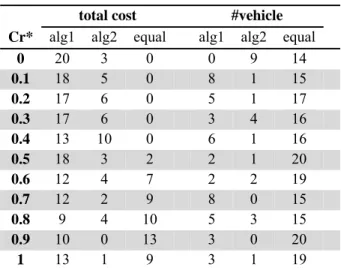
Table 1 presents a comparison between the results found by Alg1 and Alg2 for gdb files. In this table the column labeled “Cr*” shows the dispatcher preference index, column total cost is divided to three columns “alg1”, “alg2” and “equal”. The column named “alg1” gives the number of instances in which the obtained total cost by Alg1is less than the obtained total cost by Alg2. The column named “alg2” gives the number of instances in which the obtained total cost by Alg2 is less than the obtained total cost by Alg1. The column named “equal” gives the number of instances in which the total cost obtained by both Alg1 and Alg2 is equal. These three columns below the column headed “#vehicle” have the same definition but for the number of vehicle obtained by Alg1 and Alg2. As shown in table 1, the Alg1 outperforms the alg2 with respect to total cost for all dispatcher preference index values. Note that in most of instances, both Alg1 and Alg2 have equal performance with respect to the number of vehicle. However the number of instances in which the number of vehicles obtained by Alg1 is less than the number of vehicles obtained by Alg2, is more. Fig 4.a and Fig 4.b respectively illustrate both the average of total cost and the average of number
of vehicles, Alg1 is superior to Alg2. So one can conclude that the proposed new heuristic has an important effect on the final solution quality and especially on the decreasing the total cost.
Table 1 Comparison between Alg1 and Alg2 on gdb files
total cost #vehicle
Cr* alg1 alg2 equal alg1 alg2 equal
0 20 3 0 0 9 14
0.1 18 5 0 8 1 15
0.2 17 6 0 5 1 17
0.3 17 6 0 3 4 16
0.4 13 10 0 6 1 16
0.5 18 3 2 2 1 20
0.6 12 4 7 2 2 19
0.7 12 2 9 8 0 15
0.8 9 4 10 5 3 15
0.9 10 0 13 3 0 20
1 13 1 9 3 1 19
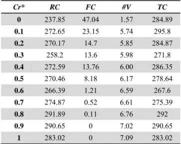
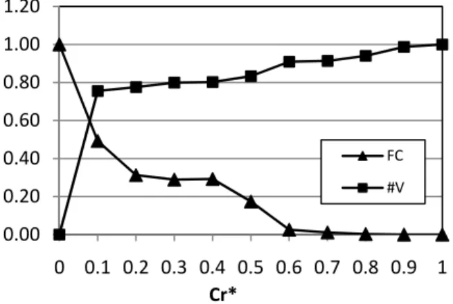
The MOMC-CARPFD before in this paper, the total cost may be reduced as the number of vehicles is increased or the total cost may be increased if the more vehicles are involved. However, the total cost includes the routing cost and the failure cost and increment or reduction of the number of vehicles effects on failure costs and consequently on routing cost. Varying values of Cr* also influences failure cost. It is prospective that the failure costs are decreased and the number of vehicles are increased as Cr*increased. It is clearly shown in table 2, that gives the results for the average of routing cost (RC), the average of failure cost (FC), the average of total cost (TC) and the average of the number of vehicles (#V) for two of the best non-dominated solutions on gdb files when the dispatcher preference index varied.The correlation between these results and Cr*are illustrated in figure 5 to figure 7. Since the values of RC, FC, TC and #V in table 2 are not of the same scale, each of them has been normalized by equation (28):
(28) Where Nr is the normalized value, is the before value, min and max are minimum and
maximum values, respectively for per RC, FC, TC and #V. Regarding compression results in table 2 and due to figure 4.a. and figure 4.b, we propose two values for dispatcher preference index:
Cr 0.3 and 0.6 because the total cost for these values is less than other values. In order to determine the final value of Cr*, the decision maker should consider some points. The lower values of Cr* conduce to the use of a less vehicle and best utilization of vehicle capacity. On the other hand, the lower values of Cr* increases the number of vehicles failing to service. Higher values of Cr* decrease the utilization of vehicle capacity along the planned route and decrease the failure cost and on the other hand the number of vehicles is increased as Cr* is increased. So the decision maker must evaluate and compare the vehicle and labor cost, vehicle capacity utilization, failure cost and total cost, then determine the value of Cr*.
Figure 4a The average total cost obtained by Alg1 and Alg2 on gdb files
Figure 4b The average number of vehicle obtained by Alg1 and Alg2 on gdb files
Table 2 The results for average RC, FC, TC and #V for different values of Cr* on gdb files
Cr* RC FC #V TC
0 237.85 47.04 1.57 284.89
0.1 272.65 23.15 5.74 295.8
0.2 270.17 14.7 5.85 284.87
0.3 258.2 13.6 5.98 271.8
0.4 272.59 13.76 6.00 286.35
0.5 270.46 8.18 6.17 278.64
0.6 266.39 1.21 6.59 267.6
0.7 274.87 0.52 6.61 275.39
0.8 291.89 0.11 6.76 292
0.9 290.65 0 7.02 290.65
1 283.02 0 7.09 283.02
265 270 275 280 285 290 295 300 305
0 0.1 0.2 0.3 0.4 0.5 0.6 0.7 0.8 0.9 1
total
cost
Cr*
Alg1 Alg2
0 2 4 6 8
0 0.1 0.2 0.3 0.4 0.5 0.6 0.7 0.8 0.9 1
Number
of
vehicles
Cr*
alg1 alg2
Figure 5 The correlation between Cr*, FC and #V
Figure 6 The correlation between Cr* and TC
Figure 7 The correlation between Cr* and RC 5.2. Results for the data set 2
In this section, we use data set 2 to investigate and compare the MOMC-CARPFD for servicing the required edges for both commodity concurrently using multi-compartment vehicles and MOMC-CARPFD for servicing the required edges for each commodity separately with single-compartment vehicles. We suppose the total vehicle capacity in both routing conditions is equal to and for concurrent servicing policy, is divided into and such that 2 and . We solve both A and B instances 10 times by Alg2 for different values of Cr* in [0,1] with step 0.2. At the end of 10 runs, two of the best solutions of non-dominated set rank 1 for each objective are
0.00 0.20 0.40 0.60 0.80 1.00 1.20
0 0.1 0.2 0.3 0.4 0.5 0.6 0.7 0.8 0.9 1 Cr*
FC #V
0.00 0.20 0.40 0.60 0.80 1.00 1.20 1.40
0 0.1 0.2 0.3 0.4 0.5 0.6 0.7 0.8 0.9 1
Norm
alized TC
Cr*
0.0 0.2 0.4 0.6 0.8 1.0 1.2
0 0.1 0.2 0.3 0.4 0.5 0.6 0.7 0.8 0.9 1
Normalized
routing
cost
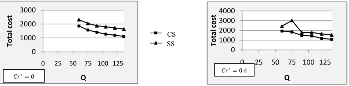
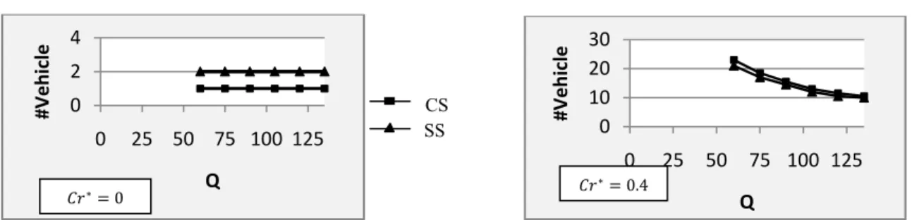
selected. Then the average for each objective is calculated. We analyze both routing policy for six values of : 60, 75, 90, 105, 120 and 135. Figure 8.a shows an example of the average total cost curves for concurrent-servicing (CS) and for separate-servicing (SS) for “A” instance and figure 8.b shows the same results for “B” instance. These figures denote that the total cost is less when two-compartment vehicles are used to serve the required edges for both commodities simultaneously beside when the unpartitioned vehicles serve the required edges per commodity separately. In general, the average of the number of vehicles obtained by separate-servicing policy is less than the average of the number of vehicles obtained by concurrent-servicing policy. However, for higher dispatcher preference index and also for higher vehicle capacity, the number of vehicles used for both routing policy is close to each other and even in some cases is equal. The figure 9.a and figure 9.b demonstrate this fact. As it can see in figure 9.b, When 0, two vehicles are used in separate-servicing policy, each vehicle services the required edges for each commodity. But in concurrent-servicing policy, since the required edges are served for both commodities simultaneously, so when 0, one vehicle is used, but on the other hand, the failure cost is more compared with separate-servicing policy.
Figure 8a Total cost for CS and SS for instance “A”
Figure 8b Total cost for CS and SS for instance “B”
Figure 9a Number of vehicle for CS and SS for instance “A”
0 1000 2000 3000 4000
0 25 50 75 100 125
Total cost Q SS CS
0 1000 2000 3000
0 25 50 75 100 125
Total
cost
Q
0 0.4
0 500 1000 1500
0 25 50 75 100 125
Total cost Q 0.4
0 500 1000 1500
0 25 50 75 100 125
Total cost Q 0 SS CS
0 1 2 3
0 25 50 75 100 125
#Vehicle Q 0
0 5 10 15
0 25 50 75 100 125
#Vehicle
Q 0.4
SS CS
Figure 9b Number of vehicle for CS and SS for instance “B” 6. CONCLUSION
In this paper, we present a new model and solution approach for more realistic CARP that is multi-objective multi-commodity capacitated arc routing problem with fuzzy demand (MOMC-CARPFD). A fuzzy chance constrained programming mathematical model was proposed based on credibility measure. In the proposed model, each required edge has demand for more than one type of commodity and also all demands for each commodity are supposed to be fuzzy numbers. Then a multi-objective genetic algorithm based on Pareto optimal set was developed to solve it, focusing on total travel cost minimization and total number of vehicle used minimization. Since the exact demand is unknown until vehicle reach to required edges, we use stochastic simulation and compute the total failure cost for planed routes. We also proposed a new heuristic to improve the initial solutions in initial population of genetic algorithm. To evaluate the new proposed model and solution approach, some data sets with fuzzy demand generated randomly are used. The computational results on date set 1 (gdb files) showed that the new heuristic has important influence on the quality of final solutions, especially on the total cost. Also the effectiveness of Cr* on final results was shown by varying its value in interval [0,1] by step 0.1. We proposed two values of dispatcher preference index; however, an advance research should be done to investigate whether these values are appropriate in other cases. In order to better analyze and compare the concurrent-servicing policy and separate-concurrent-servicing policy, we solve the MOMC-CARPFD on randomly generated instances in which the required edges have demand for two commodities (data set 2). The computational results showed that the total cost is less when two-compartment vehicle is used to servicing the required edges for two commodities concurrently. While applying separate-servicing, the number of vehicles in most cases is less compare with concurrent-servicing policy. Also the results showed that for both routing policies, the total cost and the number of vehicles is decreased as vehicle capacity increased.
In addition, four contributions of the paper can be highlighted: 1)To handle more realistic situations, we investigate the multi-objective capacitated arc routing with multi-commodities and demands uncertainty.2)We present fuzzy chance constrained model based on credibility with objectives: minimizing total travel cost and number of vehicles.3)We develop multi-objective genetic algorithm using Pareto ranking, and hybrid with stochastic simulation to design an efficient solution method.4)To improve quality of final solutions, we propose a new heuristic to generate a good initial solution for GA.
REFERENCES
[1] Beullens P., Muyldermans L., CattrysseD.,VanOudheusden D. (2003), A guided local search heuristic for the capacitated arc routing problem; European Journal of Operational Research 147(3); 629–643.
0 2 4
0 25 50 75 100 125
#Vehicle
Q 0
0 10 20 30
0 25 50 75 100 125
#Vehicle
Q 0.4
SS CS
[2] Christiansen C.H., Lysgaard J., Wøhlk S. (2009), A Branch-and-Price Algorithm for the Capacitated Arc Routing Problem with Stochastic Demands; Operations Research Letters 37; 392-398.
[3] Coello C.A.C. (1999), A Comprehensive Survey of Evolutionary-Based Multiobjective Optimization Techniques; Knowledge and Information Systems 1(3); 269–308.
[4] DeArmon J.S. (1981),A comparison of heuristics for the capacitated chinese postman problem; Dissertation, University of Maryland.
[5] Deb K., Pratap A., Agarwal S., Meyarivan T. (2002), A fast and elitist multiobjective genetic algorithm: NSGA-II; IEEE Transactions on Evolutionary Computation 6(2); 182–197.
[6] Dijkgraaf E., Gradus R. (2007), Fair competition in the refuse collection market; Applied Economic Letters 14(10); 701–704.
[7] Dijkstra E.W. (1959), A note on two problems in connection with graphs; NumerischeMathematik 1(1); 269–271.
[8] Dror M., Stern H.I. (1979), Routing Electric Meter Readers; Computers and Operations Research 6(4); 209–223.
[9] Dror M., Levy L. (1986), A vehicle routing improvement algorithm comparison of a greedy and a matching implementation for inventory routing; Computer and Operation Research 13(1); 33–45. [10] Eglese R.W., Li L. (1992), Efficient Routing for Winter Gritting; Journal of Operational Research
Society 43(11); 1031–1034.
[11] Fleury G., Lacomme,P., Prins C. (2004), Evolutionary algorithms for stochastic arc routing problems,.In: Raidl G.R., Rothlauf F., Smith G.D., Squillero G., Cagnoni S., Branke J., Corne D.W., Drechsler R., Jin Y., Johnson C.G. (Eds.), Applications of Evolutionary Computing, Springer-Verlag: Berlin; 501-512.
[12] Fleury G., Lacomme P., Prins C., Sevaux M. (2005), A memetic algorithm for a bi-objective and stochastic CARP; Multi Objective Combinatorial Optimization, The 6th Metaheuristics International Conference; 22-26.
[13] Garcia-Najera A., Bullinaria J.A. (2009), Bi-objective optimization for the vehicle routing problem with time windows: using route similarity to enhance performance, In: Ehrgott M., Fonseca C., Gandibleux X., Hao J.K., Sevaux M., editors; Proceedings of fifth international conference on evolutionary multi- criterion optimization, Lecture Notes in Computer Science 5467; 275–89.
[14] Garcia-Najera A.,Bullinaria J.A. (2011), An improved multi-objective evolutionary algorithm for the vehicle routing problem with time windows; Computers and Operation Research 38(1); 287-300. [15] Gen M., Cheng R.W. (2000), Genetic algorithms and engineering optimization; John wiley&Sons;
NewYourk.
[16] Goldberg D.E. (1989), Genetic Algorithms in Search, Optimization and Machine Learning; Addison Wesley.
[17] Goldberg D.E., Deb K. (1991), A comparative analysis of selection schemes used in genetic algorithms; In: Foundations of genetic algorithms, Morgan Kaufmann publisher; 69–93.
[18] Golden B.L., Wong R.T. (1981), Capacitated arc routing problems; Networks 11; 305–315.
[19] Golden B.L., DeArmon J.S., Baker E.K. (1983), Computational experiments with algorithms for a class of routing problems; Computers and Operations Research 10; 47–59.
[20] Grandinetti1 L., Guerriero F., Lagana D., Pisacane O. (2010), An approximate e-constraint method for the Multi-objective Undirected Capacitated Arc Routing Problem; Lecture Notes in Computer Science6049; 214-255.
[21] Greistorfer P. (2003), A Tabu Scatter Search Metaheuristic for the Arc Routing Problem; Computers and Industrial Engineering 44(2); 249–266.
[22] Han H.S., Yu J.J., Park C.G., Lee J. G. (2004), Development of inspection gauge system for gas pipeline; Korean Society Mechanical Engineering International Journal 18(3); 370–378.
[23] Hertz A., Laporte G., Mittaz M. (2000), Atabu search heuristic for the capacitated arc routing problem; Operations Research 48(1); 129–135.
[24] Hertz A., Mittaz M. (2001), A variable neighborhood descent algorithm for the undirected capacitated arc routing problem; Transportation Science 35(4); 425–434.
[25] Kaufmann A., Gupta M.M. (1985), Introduction to Fuzzy Arithmetic, Theory and Applications; Van Nostrand Reinhold, New York.
[26] Labelle A., Langevin A., Campbell J.F. (2002), Sector design for snow removal and disposal in urban areas; Socio-Economic Planning Sciences 36(3); 183–202.
[27] Lacomme P., Prins C., Ramdane-CherifW. (2004), Competitive memetic algorithms for arc routing problems; Annals of Operation Research 131; 159–185.
[28] Lacomme P., Prins C., Sevaux M. (2006), A genetic algorithm for a biobjective capacitated arc routing problem; Computers and Operations Research 33(12); 3473–3493.
[29] Liu B. (2006), A survey of credibility theory; Fuzzy Optimization and Decision Making 5(4); 387-408. [30] Mei Y., Tang K., Yao X. (2010), Capacitated arc routing problem in uncertain environments; IEEE
world congress on Computational Intelligence; Spain, 1400-1407.
[31] Mei Y., Tang K., Yao X. (2011), Decomposition-Based Memetic Algorithm for Multi-Objective Capacitated Arc Routing Problem; IEEE Transactions on Evolutionary Computation15(2);151-16. [32] Mitra K. (2009), Multiobjective optimization of an industrial grinding operation under uncertainty;
Chemical Engineering Science 64; 5043-5056.
[33] Muyldermans L., Pang G. (2010), A guided local search procedure for the multi-compartment capacitated arc routing problem, Computers and Operations Research 37; 1662–1673.
[34] Potvin J.Y., Bengio S. (1996), The vehicle routing problem with time windows, part II: Genetic search;Informs Journal of Computing 8(2); 165–172.
[35] Santos L., Coutinho-Rodrigues J.R., Current J.R. (2009), An improved heuristic for the capacitated arc routing problem; Computers and OperationsResearch 36(9); 2632–2637.
[36] Tang K., Mei Y., Yao X. (2009), Memetic Algorithm with Extended Neighborhood Search for Capacitated Arc Routing Problems; IEEE Transactions on Evolutionary Computation 13(5); 1151-1166.
[37] Tobin G.A., Brinkmann R. (2002), The effectiveness of street sweepers in removing pollutants from road surfaces in Florida; Journal of Environmental Science and Health (Part A) 37(9); 1687–1700. [38] Ulusoy G. (1985), The fleet size and mix problem for capacitated arc routing; European Journal of
Operational Research 22; 329–37.
[39] Van Veldhuizen D.A. (1999), Multiobjective Evolutionary Algorithms: Classifications, Analyses, and New Innovations; Ph.D. thesis, AFIT/DS/ENG/99-01, Air Force Institute of Technology, Wright-Patterson AFB, Ohio.
[40] Van Veldhuizen D.A., Lamont G.B. (2000), Multiobjective evolutionary algorithms: Analyzing the state-of-the-art; Evolutionary Computation 8(2); 125-147.
[41] Wøhlk S. (2005), Contributins to arc routing; PhD thesis, University of Southern Denmark. [42] Zadeh L.A. (1965), Fuzzy Sets; Information and Control 8; 338-353.