Dose distribution evaluation of various dose
calculation algorithms in inhomogeneous media
INTRODUCTION
In radiation therapy, the accuracy of dose calculations is important and of great interest to many researchers because of the presence of heterogeneous media in the human body, such
calculation algorithms are used to process and correct primary and secondary energy transfers. Radiation treatment planning (RTP) systems can be used to calculate the dose distribution and volume because tumors and normal tissue are irradiated by high-energy photons. The software
Y.L. Kim
1,2, T.S. Suh
1,2*, B.Y. Choe
1,2, B.O. Choi
3, J.B. Chung
4, J.W. Lee
5,
Y.K. Bae
5, B.M. Park
5, J.Y. Jung
6, Y.J. Shin
6, J.Y. Kim
7, S.K. Moon
11Department of Radiology, Choonhae College of Health Science, Ulsan 689-784, South Korea 2Deparement of Biomedical Engineering, The Catholic University, Seoul 137-701, South Korea
3Department of Radiation Oncology, Seoul St. Mary’s Hospital, The Catholic University, Seoul 137-701, South Korea 4Department of Radiadion Oncology, Seoul National University Bundang Hospital, Seongnam 463-707, South
Korea
5Department of Radiation Oncology, Konkuk University Medical Center, Seoul 143-729, South Korea 6Department of Radiation Oncology, Inje University Sanggye Paik Hospital, Seoul 139-707, South Korea 7Department of Radiation Oncology, Inje University Haeundae Paik Hospital, Busan 612-896, South Korea
ABSTRACT
Background: Dose calcula on algorithms play a very important role in predic ng the explicit dose distribu on. We evaluated the percent depth dose (PDD), lateral depth dose profile, and surface dose volume histogram in inhomogeneous media using calcula on algorithms and inhomogeneity correc on methods. Materials and Methods: The homogeneous and inhomogeneous virtual slab phantoms used in this study were manufactured in the radia on treatment planning system to represent the air, lung, and bone density with planned radia on treatment of 6 MV photons, a field size of 10 × 10 cm2, and a source-to-surface distance of 100 cm.Results: The PDD of air density slab for the Acuros XB (AXB) algorithm was differed by an average of 20% in comparison with other algorithms. Rebuild up occurred in the region below the air density slab (10–10.6 cm) for the AXB algorithm. The lateral dose profiles for the air density slab showed rela vely large differences (over 30%) in the field. There were large differences (20.0%–26.1%) at the second homogeneous–inhomogeneous junc on (depth of 10 cm) in the field for all calcula on methods. The surface dose volume histogram for the pencil beam algorithm showed a response that was approximately 4% lower than that for the AXB algorithm. Conclusion: The dose calcula on uncertain es were shown to change at the interface between different densi es and in varied densi es using the dose calcula on methods. In par cular, the AXB algorithm showed large differences in and out of the field in inhomogeneous media.
Keywords: Inhomogeneous media, calculation algorithms, correction methods, PDD, dose profiles.
*Corresponding author: Dr. Tae-Suk Suh,
Fax:+ 82 2 2258 7232 E-mail: [email protected] Revised: Aug. 2015
Accepted: Sept. 2015
Int. J. Radiat. Res., October 2016; 14(4): 269-278
► Original article
DOI: 10.18869/acadpub.ijrr.14.4.269
system have rapidly improved over the last few decades because of the development of computer processing. The most recently developed dose calculation algorithm in the RTP system was developed to be able to accurately and rapidly calculate the irradiated dose and scattered irradiated volume. In particular, it can adapt to inhomogeneous areas to take into account variations in primary and secondary radiation. Dose calculation algorithms play a very important role because dose distribution in treatment planning should not only predict but also correspond with the dose distribution in the irradiated volume (1). The dose distributions and calculations in the RTP system should demonstrate high accuracy and speed because the irradiated dose distribution in patients approximately corresponds to the dose calculated by the algorithms. The accuracy and speed of the RTP system are dependent on the dose calculation algorithms.
The limitations of dose calculation algorithms include dif$iculties in predicting electron transport in tissues with different densities. The dose calculations for inhomogeneous media also showed differences between the treatment planning dose and the irradiation dose because of the electron disequilibrium in different densities (2, 3). The reason for the dose calculation inaccuracies in inhomogeneous media was not considered the primary and scatter corrections, lateral scatter equilibrium, and rebuild up (4–6). Thus, the weak points of the conventional RTP system accurately predict the dose distribution for inhomogeneous tissue in the treatment volume (7, 8). The exact absorbed primary photon dose may be calculated, but it does not accurately consider scatter; in particular, the dose calculation accuracy is often reduced in the presence of inhomogeneous media. The dose calculation and distribution in inhomogeneous media are not accurate, because the photons interacting with the inhomogeneous media could not correctly account for the lack or excess of electron transport. The presently used dose correction and calculation methods in inhomogeneous regions have been improved by the developed dose calculation algorithms (9–12).
The pencil beam algorithm, which is a
previously used RTP algorithm, can be used to integrate the dose distribution. The dose distribution is composed the energy spread or dose kernel at a point by summing along a line in a phantom to obtain a pencil type beam over the patient surface (13). Conventional algorithms, such as the pencil beam convolution algorithm, have limitations, in that they represent the dose distribution with a lack of scatter correction in inhomogeneous media (14, 15). The pencil beam convolution algorithm uses the Batho power law (BPL), modi$ied Batho power law (MBPL), and equivalent tissue–air ratio (ETAR) to correct the inhomogeneous region in the irradiation volume. The collapsed cone convolution (CCC) algorithm supposes that the dose kernel composed the cone direction to transport, attenuation, and deposits on the axis (16, 17). With this algorithm, a deposited dose is calculated by the accumulated energy on the line passing through the center of the cone. The CCC algorithm is a three-dimensional (3D) model that is able to estimate the primary radiation and scatter in inhomogeneous media. The analytical anisotropic algorithm (AAA) was
developed to calculate the dose for inhomogeneous media more accurately than the
pencil beam algorithm (18, 19). The AAA can be evaluated more accurately for dose calculation in inhomogeneous regions (20). However, AAA calculations do not account for tissue properties and chemical combinations, and the algorithm does not accurately represent surface doses. A new algorithm was thus necessary to resolve the problems of the pencil beam algorithm and the AAA. The latest dose calculation algorithm is called the Acuros XB (AXB) algorithm, and it has been implemented in Eclipse treatment planning (Varian, Palo Alto, USA). Although the AXB algorithm has a slower calculation speed than the abovementioned conventional algorithms, it increased not only the surface dose accuracy but also dose correction in inhomogeneous media, such as the lung, bone, and air (21–23).
Several studies have compared the dose calculation accuracy of superposition convolution algorithms, such as the AAA and
CCC methods, against the pencil beam algorithm in homogeneous water and inhomogeneous
media. In this study, a deterministic dose algorithm, the AXB advanced dose calculation algorithm, is included to validate the accuracy of different dose calculation algorithms. Thus, the purpose of this study is to compare the percent depth dose (PDD) for homogeneous soft tissue density and inhomogeneous air, lung, and bone densities using the pencil beam algorithm (which uses the BPL, MBPL, and ETAR), the AAA, and the AXB algorithm. We also compared the lateral dose pro$iles at several depths to evaluate the primary and lateral scatter equilibriums. We used the surface dose (0–1 cm in depth) to evaluate the dose volume histogram using various algorithms and compare relative calculation differences on the surface.
MATERIALS
AND METHODS
Virtual phantom manufacture by radiation treatment planning system
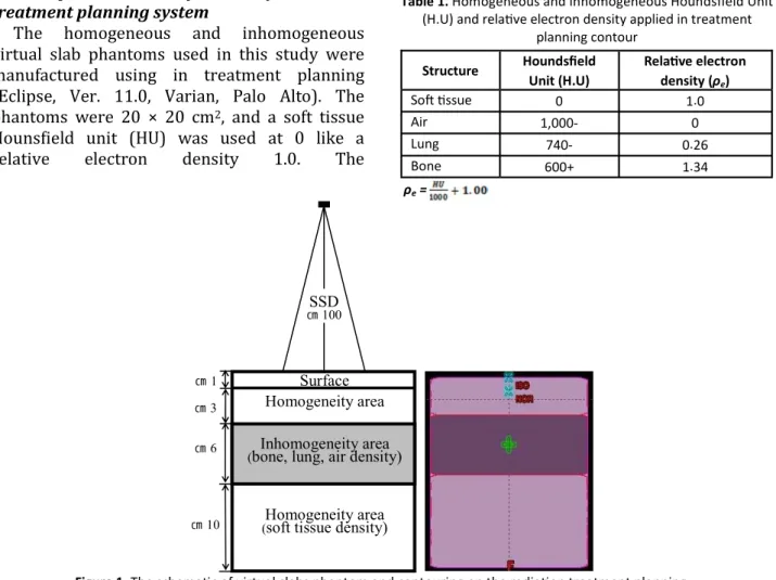
The homogeneous and inhomogeneous virtual slab phantoms used in this study were manufactured using in treatment planning (Eclipse, Ver. 11.0, Varian, Palo Alto). The phantoms were 20 × 20 cm2, and a soft tissue Houns$ield unit (HU) was used at 0 like a relative electron density 1.0. The
inhomogeneous regions were 6 cm thick with 4– 10 cm with the densities of air, lung, and bone. A soft tissue density region of 10 cm in thickness was located under the inhomogeneous region ($igure 1). The inhomogeneous density setup included layers of air (electron density 0, –1000 HU), lung (electron density 0.26, –740 HU), and bone (electron density 1.34, +600 HU) (table 1) (24). The surface area used to estimate the surface volume dose was between the surface and a depth of 1 cm.
Radiation treatment planning by various algorithms
The contoured phantoms underwent RTP with 6 MV photons, a source surface distance (SSD) of 100 cm, a $ield size of 10 × 10 cm2, and a single anterior $ield direction. The normalization point was located at Dmax, and the fraction dose was 180 cGy. The change in the tissue electron
SSD 100 ㎝
3 ㎝
6 ㎝
10 ㎝
1 ㎝
Inhomogeneity area (bone, lung, air density)
Homogeneity area
Homogeneity area (soft tissue density)
Surface
Figure 1. The schema c of virtual slabs phantom and contouring on the radia on treatment planning.
Table 1. Homogeneous and inhomogeneous Houndsfield Unit (H.U) and rela ve electron density applied in treatment
planning contour Structure Houndsfield
Unit (H.U)
Rela ve electron density (ρe)
So9 ssue 0 1.0
Air 1,000 - 0
Lung 740 - 0.26
Bone 600 + 1.34
ρe =
density in the irradiated volume resulted in a change in the PDD and the lateral depth dose pro$ile because of the photon transmission and scatter. Therefore, we compared and analyzed the differences in the electron densities in the PDD and lateral depth dose pro$ile after RTP was implemented in the homogeneous and inhomogeneous phantoms using the calculation algorithms and inhomogeneity correction methods. The pencil beam algorithm uses the
BPL, MBPL, and ETAR to correct for inhomogeneous media. The BPL method was
used for the manual calculation of one-dimensional inhomogeneity correction
before computed tomography based RTP. The MBPL formula quotes from the BPL as a 1D correction method. The BPL and MBPL under-correct for substances with densities lower than that of water and over-correct for substances with densities higher than that of water. The ETAR, which is a two-dimensional
algorithm, was the $irst practical dose calculation method using all CT data. The ETAR
includes the 3D tissue density information for accurate calculations of the dose scatter; however, the scatter decreases in densities lower than that of soft tissue and increases in
higher densities. The AAA, which is a convolution method, may offer more accurate
calculations than the pencil beam algorithm for inhomogeneous areas. The AAA calculates the beam and allows energy $luency that is composed of three separate sources: primary photons, extra focal photons, and contamination electrons (25). The AXB calculation implements the latest version of the Eclipse planning system and is similar to the Monte Carlo method. The
AXB algorithm can calculate 3D dose distributions by using the primary photon
source, scattered photon $luency, and scattered electrons.
Statistical analysis
The PDDs determined by various algorithms were compared from the surface to a depth of 18 cm to analyze the dose distribution by the
primary photons and the scatter in homogeneous and inhomogeneous media. The
average dose differences and standard deviation
were calculated by the statistical software (SPSS, Ver. 21.0, IBM). We compared the PDD at the surface (0–1 cm), the $irst homogeneous area (0–4 cm), the inhomogeneous area (4–10 cm), and the inhomogeneous and second homogeneous area (10–20 cm). The comparison of primary photons, secondary scatter, and lateral scatter due to the electron density was evaluated using the lateral depth dose pro$ile at
Dmax, the $irst homogeneous–inhomogeneous
junction (4 cm), the center of the inhomogeneous area (7 cm), and the second
homogeneous–inhomogeneous junction (10 cm). The pencil beam algorithm and AAA did not accurately re$lect the surface dose because of the lack of primary and scatter corrections. Thus, we evaluated the dose volume histogram (DVH) to analyze the surface (0–1 cm).
RESULTS
Percent depth dose comparison
The represented PDDs were calculated using the pencil beam algorithm, AAA, and AXB algorithm with 6 MV photons and a $ield size of 10 × 10 cm2 in the virtual slab phantoms at a central axis ($igure 2). The pencil beam algorithm uses the BPL, MBPL, and ETAR for inhomogeneity correction.
Table 2 shows the average and standard deviation of the PDD in the virtual slab phantoms. All PDDs in the soft tissue density were in good agreement (within 2.3%) from Dmax to a depth of 18 cm in the virtual slab phantoms when comparing the AXB algorithm with the AAA, BPL, MBPL, and ETAR. However, the surface PDD (0–1 cm) showed a relative maximum average and a standard deviation of 8.1 cGy ± 7.9 when using the ETAR. For a homogeneous phantom, the difference in PDD was largest when using the ETAR and AAA, both of which showed good agreement with the AXB algorithm (within 2.0 cGy ± 1.9). The PDD of the $irst homogeneous area (0–4 cm) yielded the maximum difference of within 2.3%. The maximum difference in the PDD of the inhomogeneous air was 22.0 cGy ± 7.0 when comparing ETAR with AXB. The average
differences in the air density were approximately 20% for other calculation methods. The PDDs for the lung and bone density slabs (4–10 cm) were showed differences within 3%. The PDD difference for the lung slab had a maximum of 2.77% for AAA and minimum of 0.5% for ETAR. It was rebuilt in the region below the air density area (10–10.6 cm) for AXB calculations ($igure 2b). However, other calculation methods did not demonstrate this rebuild up. The rebuild up region had a maximum difference of 38.1% below the air slab for ETAR, and the average difference was
approximately 10% in the second homogeneous area (10–20 cm) for all methods. The bone density slab yielded the lowest difference in the PDD in the second homogeneous area for all calculation algorithms.
Lateral depth dose pro"ile and surface dose volume histogram
The lateral depth dose pro$iles for the AXB algorithm, AAA, BPL, ETAR, and MBPL are given at Dmax, the $irst homogeneous–inhomogeneous junction (4 cm), the center of the inhomogeneous region (7 cm), and the second
Figure 2. Percent depth dose in (a) so9 ssue, (b) air, (c) lung, and (d) bone density slab phantom for Acuros XB algorithm, analy cal anisotropic algorithm, and Pencil beam algorithm (Batho Power, Modified Batho power, equivalent ssue air ra o).
surface
(0~1 cm)
Homogeneity area (0~4 cm)
Inhomogeneity area (4~10 cm)
Homogeneity area (10~20 cm) Inhomogeneity
media
Calcula on
method Avg.±SD (cGy) Avg.±SD (cGy) Avg.±SD (cGy) Avg.±SD (cGy) Air
density (ρe=0)
AAA 0.8 ± 0.7 0.4 ± 0.5 20.1 ± 6.8 11.9 ± 14.6
M.Batho 6.3 ± 8.4 1.8 ± 4.8 20.7 ± 6.2 10.9 ± 15.0
ETAR 8.0 ± 8.0 2.1 ± 5.1 22.0 ± 7.0 12.1 ± 16.1
Batho 6.3 ± 8.4 1.8 ± 4.8 20.0 ± 5.1 10.2 ± 13.3
Lung density (ρe=0.26)
AAA 1.3 ± 0.9 0.5 ± 0.6 2.8 ± 0.6 1.7 ± 1.1
M.Batho 5.9 ± 8.8 1.6 ± 4.8 0.7 ± 0.2 0.6 ± 0.2
ETAR 7.4 ± 8.4 1.9 ± 5.1 0.5 ± 0.4 1.2 ± 0.5
Batho 5.9 ± 8.8 1.6 ± 4.8 1.3 ± 1.1 1.9 ± 0.8
Table 2. Percent depth dose difference between Acuros XB and various calcula on methods (analy cal anisotropic algorithm, Batho Power law, Modified Batho Power law, equivalent ssue air ra o) in the virtual slabs inhomogeneous phantom
(a) (b)
(c) (d)
homogeneous–inhomogeneous junction (10 cm) ($igure 3). All depth dose pro$iles were in good agreement (within 1.5%) in the 10 × 10 cm2 $ield at Dmax. However, the dose pro$iles in out of the $ield showed relatively large differences in their maximum averages and standard deviations (13.6 cGy ± 23.9) for the BPL. The AAA calculations were in good agreement with the AXB algorithm (within 1.9 cGy ± 6.4) in and out of the $ield at Dmax.
Tables 3 and 4 give the averages and standard deviations for the lateral depth dose pro$iles in the virtual slab phantoms at several depths. The
results for the soft tissue density slab were within 1% at all depths in the $ield region for all calculation algorithms. The dose pro$iles out of the $ield showed a relatively large discrepancy to the process sequence BPL, ETAR, and MBPL in the soft tissue density phantom, but that of the AAA was in good agreement with the AXB algorithm (within 1.2 cGy ± 3.2). The results of the $irst junction in the $ield were within 1.3 cGy ± 1.13 and 1.2 cGy ± 1.93 in the bone and lung density slabs, respectively. For the air density slab, the dose pro$iles in the $ield showed slightly higher differences (2.1%–4.3%), with a
(a) (b)
(c) (d)
Figure 3. Lateral depth dose profiles (a) so9 ssue, (b) air, (c) lung, and (d) bone density slab phantom for Acuros XB algorithm, analy cal anisotropic algorithm, and Pencil beam algorithm (Batho Power, Modified Batho power, equivalent.
Table 3. Infield lateral dose profile difference between Acuros XB and various calcula on methods (analy cal anisotropic algorithm, Batho Power law, Modified Batho Power law, equivalent ssue air ra o) in the virtual slabs inhomogeneous phantom
Dmax 4 cm 7 cm 10 cm
Inhomogeneity media Calcula on method Avg.±SD (cGy) Avg.±SD (cGy) Avg.±SD (cGy) Avg.±SD (cGy) Air density
(ρe=0)
AAA 0.5 ± 2.0 2.1 ± 0.6 33.8 ± 4.2 24.1 ± 5.6
M.Batho 1.4 ± 4.1 4.3 ± 1.8 34.1 ± 4.6 23.6 ± 5.7
ETAR 0.4 ± 1.1 3.2 ± 0.3 35.8 ± 3.9 26.1 ± 5.3
Batho 1.2 ± 3.8 4.3 ± 1.6 30.9 ± 4.5 20.0 ± 5.7
Lung density (ρe=0.26)
AAA 1.5 ± 5.0 1.0 ± 1.4 2.6 ± 1.0 1.6 ± 0.5
M.Batho 0.4 ± 1.2 1.2 ± 1.5 2.1 ± 3.2 1.2 ± 1.8
ETAR 0.8 ± 2.6 1.0 ± 2.1 3.7 ± 3.8 3.6 ± 2.0
Batho 0.6 ± 2.2 1.2 ± 1.9 2.8 ± 2.5 1.9 ± 1.0
maximum difference of 8.7% out of the $ield for the MBPL. The results for the center of the inhomogeneous density slab in the $ield showed slight differences (2.1%–3.7%) for the bone and lung densities for all calculation methods. However, the dose pro$iles for the air density slab showed a relatively large difference of over 30%, and the maximum discrepancy was 35.8 ± 3.88 for the ETAR. The differences out of the $ield were relatively small (within 9.4%) in comparison to those in the $ield. There were large differences (20.0%–26.1%) at the second homogeneous–inhomogeneous junction (10 cm)
in the $ield for all calculation methods. The results of the second junction for the bone and lung density slabs showed small differences (within about 3.6%) in the $ield. All lateral dose pro$iles in and out of the $ield represented over-calculated doses in comparison with those calculated using the AXB algorithm.
For the pencil beam algorithm, the surface dose volume histogram showed approximately 4% lower responses than the AXB algorithm. The surface dose volume histogram of the AAA was in good agreement with the AXB algorithm (within –0.3%) ($igure 4).
Table 4. Out of field lateral dose profile difference between Acuros XB and various calcula on methods (analy cal anisotropic algorithm, Batho Power law, Modified Batho Power law, equivalent ssue air ra o) in the virtual slabs inhomogeneous phantom.
Dmax 4 cm 7 cm 10 cm
Inhomogeneity media
Calcula on
method Avg.±SD (cGy) Avg.±SD (cGy) Avg.±SD (cGy) Avg.±SD (cGy)
Air density (ρe=0)
AAA 1.5 ± 3.3 1.3 ± 3.3 9.6 ± 8.2 9.4 ± 7.8
M.Batho 9.5 ± 18.6 8.6 ± 16.2 11.3 ± 13.1 9.1 ± 10.8
ETAR 3.4 ± 6.4 2.9 ± 4.9 9.3 ± 8.5 7.7 ± 7.6
Batho 8.0 ± 16.0 7.3 ± 14.0 10.4 ± 11.3 8.3 ± 8.9
Lung density (ρe=0.26)
AAA 1.9 ± 6.4 0.9 ± 2.4 0.9 ± 1.1 0.4 ± 0.6
M.Batho 4.4 ± 8.3 4.9 ± 9.5 4.0 ± 6.4 3.0 ± 5.7
ETAR 8.4 ± 16.1 8.5 ± 16.0 6.8 ± 12.0 6.8 ± 11.2
Batho 6.8 ± 13.1 7.2 ± 13.9 5.4 ± 9.2 4.8 ± 8.6
Figure 4. Dose volume histogram (DVH) at surface region (0~1 cm) for Acuros XB algorithm, analy cal anisotropic algorithm, and Pencil beam algorithm (Batho Power, Modified Batho power, equivalent ssue air ra o).
DISCUSSION
The accuracy of the dose calculation and distribution in RTP plays a very important role because it must be consistent with the dose distribution in the irradiated volume. If the accuracy of the dose in the patient can be improved by 1%, the cure rate would increase by 2% for early-stage tumors. If the tumor control dose is within 95%–107% of the dose distribution, it may be treated without complications. If changes in the tumor control dose of 5% occur, the local tumor control probability changes by 10%–20%, or the normal tissue complication probability (NTCP) changes by up to 30% (26). Therefore, the dose accuracy is very important in determining the success or failure of the treatment, and the choice of dose calculation algorithm is very important to improve the dose distribution accuracy of planning and irradiation. In particular, dose calculations vary according to the employed dose calculation algorithms, as well as the inhomogeneity correction methods if the tumor is located in an inhomogeneous region. The dose calculation algorithms and inhomogeneity correction methods used for RTP systems include the pencil beam algorithm, AAA, AXB algorithm, BPL, MBPL, and ETAR, among others. In several studies, the AXB algorithm has shown improvement in the conformity of measurements and Monte Carlo simulations during dose calculation in inhomogeneous media (5, 6).
In this study, we used the AXB algorithm, AAA, and pencil beam algorithm to evaluate the dose distribution (speci$ically, the PDD and lateral depth dose pro$ile) in homogeneous and inhomogeneous media. The virtual slab phantoms used in this study were manufactured to describe the inhomogeneous regions that can be represented by air, lung, and bone density slabs (22).
The surface PDDs (depths of 0–1 cm) were slightly higher for the AXB algorithm than those for other algorithms. Whereas the conventional calculation algorithms demonstrate low dose accuracy because of the lack of dose correction on the surface, the AXB algorithm improved the
dose correction on the surface. Thus, the surface PDD could be increased using the AXB algorithm. The PDD in the air density slab was
decreased to reduce interaction with lower-density slabs for measurements. The PDD
in the air density slab represented a similar dose distribution to that represented by measurements using the AXB algorithm due to the lack of interactions. The junction between the air and soft tissue density slabs increased the secondary electrons due to the increased interaction below the soft tissue density slab (8). The PDDs showed differences in the dose distribution within approximately 3% for the lung and bone density slabs due to the discrepancy of the corrections for primary and secondary radiation (22, 23).
The lateral depth dose pro$iles demonstrated a large difference out of the $ield (penumbra region) resulting from the increase in the lateral scatter disequilibrium between the AXB and pencil beam algorithms. The AAA yielded results similar to those of the AXB algorithm for lateral depth dose pro$iles out of the $ield. Differences in the depth dose pro$iles depending on the dose calculation methods arose because of the lack of interaction between primary and secondary radiation in the air slab phantom. There were signi$icant differences in the dose distributions determined by the AXB algorithm and conventional calculation methods at the air density center and the junction between the air and soft tissue densities. The depth dose pro$ile at the center of the air density slab showed a lower dose than at the junction between the air and soft tissue density slabs at a depth of 10 cm in the $ield because it decreased the interactions at low densities. The lateral depth dose pro$ile at the junction of the lung and soft tissue density slabs (second homogeneous–inhomogeneous junction) was higher than that at the same position in the bone or soft tissue density phantoms because it decreased the dose attenuation in the lung density slab. The AXB algorithm could improve the dose correction in the surface region, so the surface dose volume was 1%–3% higher for the AXB algorithm than the pencil beam algorithm and the AAA (27).
In general, it was determined that dose
calculation uncertainties change at the interface between different densities and in varied densities when using the dose calculation methods. The advanced dose calculation algorithm should be used in treatment planning systems for high dose calculation accuracy and dose prediction because the irradiated volumes are composed of different electron densities. In comparison with the pencil beam algorithm and the AAA, the AXB algorithm requires substantial calculation time because of the $ield size and volume density. Therefore, the dose calculation algorithm should now be further developed considering its accuracy and calculation speed.
ACKNOWLEDGMENT
This work was supported by Radiation Technology R&D program through the National Research Foundation of Korea funded by the Ministry of Science, ICT&Future Planning (No. 2013M2A2A7043498) and this research was supported by Choonhae College of Health Sciences Con"lict of interest: Declared none.
REFERENCES
1. Podgorsak EB (2005) Radia on Oncology Physics: a handbook for teachers and students. IAEA, Vienna
2. Engelsman M, Damen EMF, Koken PW, Koken, Veld AA, Ingen KM, Mijnheer BJ (2001) Imfact of simple ssue inhomogeneity correc on algorithms on conformal radiotherapy of lung tumors. Radiother Oncol, 60: 299-309.
3. Shahine B, Al-Ghazi M, El-Kha b E (1999) Experimental evalua on of interface doses in the presence of air cavi es compared with treatment planning algorithms. Med Phys,
26: 350-355.
4. Gete E, Teke T, Kwa W (2012) Evalua on of AAA treatment planning algorithm for SBRT lung treatment: comparison with Monte Carlo and homogeneous pencil beam dose calcula on. Journal of Medical Imaging and Radia on Sciences, 43: 26-33.
5. Han T, Mikell JK, Salehpour M, Mourtada F (2011) Dosimetric comparison of Acuros XB determinis c radia on transport method with Monte Carlo and model-based convolu on methods in heterogeneous media. Med
Phys, 38: 2651-2664.
6. Bush K, Gagne IM, Zavgorodni S, Ansbacher W, Beckham W (2011) Dosimetric valida on of Acuros XB with Monte Carlo methods for photon dose calcula ons. Med Phys,
38: 2208-2221.
7. Papanikolaou N and Stathakis S (2009) Dose-calcula on algorithms in the context of inhomogeneity correc ons for high energy beams. Med Phys, 36: 4765-4775.
8. Kim YL, Suh TS, Ko SG, Lee JW (2010) Comparison of experimental and radia on therapy planning dose distribu on on air cavity. Journal of Radiological Science
and Technology, 33: 261-268.
9. Mohan R, Chui C, Lidofsky L (1986) Differen al pencil beam dose computa on model for photons calcula ons. Med Phys, 13: 64-73.
10. Boyer AL, Zhu YP, Wang L, Francois P (1989) Fast Fourier transform convolu on calcula ons of x-ray dose distribu ons inhomogeneous media. Med Phys, 16: 248-253.
11. Ahnesjo A (1989) Collapsed cone convolu on of radiant energy for photon dose calcula on in heterogeneous media. Med Phys, 16: 577-592.
12. Hansenbalg F, Neuenschwander H, Mini R, Born EJ (2007) Collapsed cone convolu on and analy cal anisotropic algorithm dose calcula ons compared to VMC++ Monte Carlo simula ons in clinical cases. Phys Med Biol, 52: 3679-3691.
13. Buzdar SA, Afzal M, Pokropek A (2010) Comparison of pencil beam ad collapsed cone algorithms, in radiotherapy treatment planning for 6 and 10 MV photon. J Ayub Med
Coll Abbo-abad, 22: 152-154.
14. Papanikolaou N, BaOsta J, Boyer AL (2004) Tissue inhomogeneity correc on for megavoltage photon beams. The report of Task Group No. 65 of the Radia on Therapy commiPee of the AAPM.
15. Kang SK, Ahn SH, Kim CY (2011) A study on photon dose calcula on in 6MV linear accelerator based on Monte Carlo method. Journal of Radiological Science and
Technology, 34: 43-50.
16. Jung JY, W Cho, Kim MJ, Lee JW (2012) Evalua on of beam modeling using collapsed cone convolu on algorithm for dose calcula on in radia on therapy planning system.
Progress in Medical Physics, 33:188-198.
17. Baghani. HR, Aghamiri SMR, Gharaa H, Mahdavi SR, Hosseini Daghigh SM (2011) Comparing the results of 3D treatment planning and prac cal dosimetry in craniospinal radiotherapy using Rando phantom. Int J Radiat Res, 9:
151-158.
18. Robinson D (2008) Inhomogeneity correc on and the analy c anisotropic algorithm. JACMP, 9: 112-122.
19. Breitman K, Rathee S, Fallone G (2007) Experimental valida on of the Eclipse AAA algorithm. JACMP, 8: 76-92. 20. Sterpin E, Tomsej M, De Smedt B, Reynaert N, Vynckier S
(2007) Monte Carlo evalua on of the AAA treatment planning algorithm in a heterogeneous mul layer phantom and IMRT clinical treatments for an Elekta SL 25 linear accelerator. Med Phys, 34: 1665-1677.
21. Failla GA, Wareing T, Archambault Y (2010) Acuros XB
advanced dose calcula on for the Eclipse treatment planning system. Varian Medical System Palo Alto.
22. Fogiata A, Nicolini G, Clivio A, VaneO E, Cozzi L (2011) Dosimetric evalua on of Acuros XB advanced dose calcula on algorithm in heterogeneous media. Radia on Oncology, 6: 82.
23. Rana S and Rogers K (2013) Dosimetric evalua on of Acuros XB dose calcula on algorithm with measurements in predic ng doses beyond different air gap thickness for smaller and larger field sizes. Med Phys, 38: 9-14.
24. Thomas SJ (1999) Rela ve electron density calibra on of CT scanners for radiotherapy treatment planning. The
Bri sh Journal of Radiology, 72:781-786.
25. Sievinen J, Ulmer W, Kaissl W (2005) AAA photon dose calcula on model in Eclipse. Varian Medical System. Palo Alto.
26. ChePy IJ, Curran B, Cygler JE, EdMarco JJ, Ezzell G (2007) Report of the AAPM Task Group No. 105: Issues associated with clinical implementa on of Monte Carlo-based photon and electron external beam treatment planning. Med Phys,
34: 4818-4853.
27. Jarkko O (2014) The accuracy of the Acuros XB algorithm in external beam radiotherapy. Int J cancer therapy and oncology, 2: 83-87.