EVALUATION OF GAUSSIAN PROCESSES AND OTHER METHODS FOR NON-LINEAR REGRESSION. Carl Edward Rasmussen

(1)

EVALUATION OF GAUSSIAN PROCESSES AND

OTHER METHODS FOR NON-LINEAR REGRESSION

Carl Edward Rasmussen

A thesis submitted in conformity with the requirements for the degree of Doctor of Philosophy,

Graduate Department of Computer Science, in the University of Toronto

c

(2)

Evaluation of Gaussian Processes and

other Methods for Non-Linear Regression

Carl Edward Rasmussen

A thesis submitted in conformity with the requirements for the degree of Doctor of Philosophy,

Graduate Department of Computer Science, in the University of Toronto

Convocation of March 1997

Abstract

This thesis develops two Bayesian learning methods relying on Gaussian processes and a rigorous statistical approach for evaluating such methods. In these experimental designs the sources of uncertainty in the estimated generalisation performances due to both vari-ation in training and test sets are accounted for. The framework allows for estimvari-ation of generalisation performance as well as statistical tests of significance for pairwise compar-isons. Two experimental designs are recommended and supported by the DELVE software environment.

Two new non-parametric Bayesian learning methods relying on Gaussian process priors over functions are developed. These priors are controlled by hyperparameters which set the characteristic length scale for each input dimension. In the simplest method, these parameters are fit from the data using optimization. In the second, fully Bayesian method, a Markov chain Monte Carlo technique is used to integrate over the hyperparameters. One advantage of these Gaussian process methods is that the priors and hyperparameters of the trained models are easy to interpret.

The Gaussian process methods are benchmarked against several other methods, on regres-sion tasks using both real data and data generated from realistic simulations. The ex-periments show that small datasets are unsuitable for benchmarking purposes because the uncertainties in performance measurements are large. A second set of experiments provide strong evidence that the bagging procedure is advantageous for the Multivariate Adaptive Regression Splines (MARS) method.

The simulated datasets have controlled characteristics which make them useful for under-standing the relationship between properties of the dataset and the performance of different methods. The dependency of the performance on available computation time is also inves-tigated. It is shown that a Bayesian approach to learning in multi-layer perceptron neural networks achieves better performance than the commonly used early stopping procedure, even for reasonably short amounts of computation time. The Gaussian process methods are shown to consistently outperform the more conventional methods.

(3)

Acknowledgments

Many thanks to Radford Neal and Geoffrey Hinton for sharing their insights and enthusiasm throughout my Ph.D. work. I hope that one day I will similarly be able to inspire people around me.

I also wish to thank past and present members and visitors to the neuron and DELVE groups as well as my committee, in particular Drew van Camp, Peter Dayan, Brendan Frey, Zoubin Ghahramani, David MacKay, Mike Revow, Rob Tibshirani and Chris Williams. Thanks to the Freys and the Hardings for providing me with excellent meals at times when my domestic life was at an ebb. Lastly, I wish to thank Agnes Heydtmann for her continued encouragement and confidence.

During my studies in Toronto, I was supported by the Danish Research Academy, by the University of Toronto Open Fellowship and through grants to Geoffrey Hinton from the Na-tional Sciences and Engineering Research Council of Canada and the Institute for Robotics and Intelligent Systems.

(4)

Introduction

The ability to learn relationships from examples is compelling and has attracted interest in many parts of science. Biologists and psychologists study learning in the context of animals interacting with their environment; mathematicians, statisticians and computer scientists often take a more theoretical approach, studying learning in more artificial contexts; people in artificial intelligence and engineering are often driven by the requirements of technolog-ical applications. The aim of this thesis is to contribute to the principles of measuring performance of learning methods and to demonstrate the effectiveness of a particular class of methods.

Traditionally, methods that learn from examples have been studied in the statistics commu-nity under the names of model fitting and parameter estimation. Recently there has been a huge interest in neural networks. The approaches taken in these two communities have differed substantially, as have the models that are studied. Statisticians are usually con-cerned primarily with interpretability of the models. This emphasis has led to a diminished interest in very complicated models. On the other hand, workers in the neural network field have embraced ever more complicated models and it is not unusual to find applications with very computation intensive models containing hundreds or thousands of parameters. These complex models are often designed entirely with predictive performance in mind.

Recently, these two approaches to learning have begun to converge. Workers in neural networks have “rediscovered” statistical principles and interest in non-parametric modeling has risen in the statistics community. This intensified focus on statistical aspects of non-parametric modeling has brought an explosive growth of available algorithms. Many of

(8)

2 Introduction

these new flexible models are not designed with particular learning tasks in mind, which introduces the problem of how to choose the best method for a particular task. All of these general purpose methods rely on various assumptions and approximations, and in many cases it is hard to know how well these are met in particular applications and how severe the consequences of breaking them are. There is an urgent need to provide an evaluation of these methods, both from a practical applicational point of view and in order to guide further research.

An interesting example of this kind of question is the long-standing debate as to whether Bayesian or frequentist methods are most desirable. Frequentists are often unhappy about the setting of priors, which is sometimes claimed to be “arbitrary”. Even if the Bayesian theory is accepted, it may be considered computationally impractical for real learning prob-lems. On the other hand, Bayesians claim that their models may be superior and may avoid the computational burden involved in the use of cross-validation to set model complexity. It seems doubtful that these disputes will be settled by continued theoretical debate. Empirical assessment of learning methods seems to be the most appealing way of choosing between them. If one method has been shown to outperform another on a series of learning problems that are judged to be representative, in some sense, of the applications that we are interested in, then this should be sufficient to settle the matter. However, measuring predictive performance in a realistic context is not a trivial task. Surprisingly, this is a tremendously neglected field. Only very seldom are conclusions from experimental work backed up by statistically compelling evidence from performance measurements.

This thesis is concerned with measuring and comparing the predictive performance of learn-ing methods, and contains three main contributions: a theoretical discussion of how to perform statistically meaningful comparisons of learning methods in a practical way, the introduction of two novel methods relying on Gaussian processes, and a demonstration of the assessment framework through empirical comparison of the performance of Gaussian process methods with other methods. An elaboration of each of these topics will follow here.

I give a detailed theoretical discussion of issues involved in practical measurement of pre-dictive performance. For example, many statisticians have been uneasy about the fact that many neural network methods involve random initializations, such that the result of learn-ing is not a unique set of parameter values. However, once these issues are faced it is not difficult to give them a proper treatment. The discussion involves assessing the statistical significance of comparisons, developing a practical framework for doing comparisons and

(9)

3

measures ensuring that results are reproducible. The focus of Chapter 2 is to make the goal of comparisons precise and to understand the uncertainties involved in empirical evalua-tions. The objective is to obtain a good tradeoff between the conflicting aims of statistical reliability and practical applicability of the framework to computationally intensive learning algorithms. These considerations lead to some guidelines for how to measure performance. A software environment which implements these guidelines called DELVE — Data for Eval-uating Learning in Valid Experiments — has been written by our research group headed by Geoffrey Hinton. DELVE is freely available on the world wide web1. DELVE contains the software necessary to perform statistical tests, datasets for evaluations, results of ap-plying methods to these datasets, and precise descriptions of methods. Using DELVE one can make statistically well founded simulation experiments comparing the performance of learning methods. Chapter 2 contains a discussion of the design of DELVE, but implemen-tational details are provided elsewhere [Rasmussen et al. 1996].

DELVE provides an environment within which methods can be compared. DELVE in-cludes a number of standardisations that allow for easier comparisons with earlier work and attempts to provide a realistic setting for the methods. Most other attempts at mak-ing benchmark collections provide the data in an already preprocessed format in order to heighten reproducibility. However, this approach seems misguided, if one is attempting to measure the performance that could be achieved in a realistic setting, where the prepro-cessing could be tailored to the particular method. To allow for this, definitions of methods in DELVE must include descriptions of preprocessing. DELVE provides facilities for some common types of preprocessing, and also a “default” attribute encoding to be used by researchers who are not primarily interested in such issues.

In Chapter 3 detailed descriptions of several learning methods that emphasize reproducibil-ity are given. The implementations of many of the more complicated methods involve choices that may not be easily justifiable from a theoretical point of view. For example, many neural networks are trained using iterative methods, which raises the question of how many iterations one should apply. Sometimes convergence cannot be reached within rea-sonable amount of computational effort, for example, and sometimes it may be preferable to stop training before convergence. Often these issues are not discussed very thoroughly in the articles describing new methods. Furthermore authors may have used preliminary simulations to set such parameters, thereby inadvertently opening up the possibility of bias in simulation results.

(10)

4 Introduction

In order to avoid these problems, the learning methods must be specified precisely. Methods that contain many parameters that are difficult to set should be recognized as having this handicap, and heuristic rules for setting their parameters must be developed. If these rules don’t work well in practice, this may show up in the comparative studies, indicating that this learning method would not be expected to do well in an actual application. Naturally, some parameters may be set by some initial trials on the training data, in which case this would be considered a part of the training procedure. This precise level of specification is most easily met for “automatic” algorithms, which do not require human intervention in their application. In this thesis only such automatic methods will be considered.

The methods described in Chapter 3 include methods originating in the statistics com-munity as well as neural network methods. Ideally, I had hoped to find descriptions and implementations of these methods in the literature, so that I could concentrate on testing and comparing them. Unfortunately, the descriptions found in the literature were rarely detailed enough to allow direct application. Most frequently details of the implementations are not mentioned, and in the rare cases where they are given they are often of an un-satisfactory nature. As an example, it may be mentioned that networks were trained for 100 epochs, but this hardly seems like a principle that should be applied universally. On the other hand it has proven extremely difficult to design heuristic rules that incorporate a researcher’s “common sense”. The methods described in Chapter 3 have been selected par-tially from considerations of how difficult it may be to invent such rules. The descriptions contain precise specifications as well as a commentary.

In Chapter 4 I develop a novel Bayesian method for learning relying on Gaussian processes. This model is especially suitable for learning on small data sets, since the computational requirements grow rapidly with the amount of available training data. The Gaussian process model is inspired by Neal’s work [1996] on priors for infinite neural networks and provides a unifying framework for many models. The actual model is quite like a weighted nearest neighbor model with an adaptive distance metric.

A large body of experimental results has been generated using DELVE. Several neural net-work techniques and some statistical methods are evaluated and compared using several sources of data. In particular, it is shown that it is difficult to get statistically significant comparisons on datasets containing only a few hundred cases. This finding suggests that many previously published comparisons may not be statistically well-founded. Unfortu-nately, it seems hard to find suitable real datasets containing several thousand cases that could be used for assessments.

(11)

5

In an attempt to overcome this difficulty in DELVE we have generated large datasets from simulators of realistic phenomena. The large size of these simulated datasets provides a high degree of statistical significance. We hope that they are realistic enough that researchers will find performance on these data interesting. The simulators allow for generation of datasets with controlled attributes such as degree of non-linearity, input dimensionality and noise-level, which may help in determining which aspects of the datasets are important to various algorithms. In Chapter 5 I perform extensive simulations on large simulated datasets in DELVE. These simulations show that the Gaussian process methods consistently outperform the other methods.

(12)

(13)

Chapter 2

Evaluation and Comparison

In this chapter I discuss the design of experiments that test the predictive performance of learning methods. A large number of such learning methods have been proposed in the literature, but in practice the choice of method is often governed by tradition, familiarity and personal preference rather than comparative studies of performance. Naturally, pre-dictive performance is only one aspect of a learning method; other characteristics such as interpretability and ease of use are also of concern. However, for predictive performance a well developed set of directly applicable statistical techniques exist that enable comparisons. Despite this, it is very rare to find any compelling empirical performance comparisons in the literature on learning methods [Prechelt 1996]. I will begin this chapter by defining generalisation, which is the measure of predictive performance, then discuss possible exper-imental designs, and finally give details of the two most promising designs for comparing learning methods, both of which have been implemented in the DELVE environment.

2.1 Generalisation

Usually, learning methods are trained with one of two goals: either to identify an inter-pretation of the data, or to make predictions about some unmeasured events. The present study is concerned only with accuracy of this latter use. In statistical terminology, this is sometimes called the expected out-of-sample predictive loss; in the neural network literature it is referred to as generalisation error. Informally, we can define this as the expected loss for a particular method trained on data from some particular distribution on a novel (test)

(14)

8 Evaluation and Comparison

case from that same distribution.

In the formalism alluded to above and used throughout this thesis the objective of learning will be to minimize this expected loss. Some commonly used loss functions are squared error loss for regression problems and 0/1-loss for classification; others will be considered as well. It should be noted that this formalism is not fully general, since it requires that losses can be evaluated on a case by case basis. We will also disallow methods that use the inputs of multiple test cases to make predictions. This confinement to fixed training sets and single test cases rules out scenarios which involve active data selection, incremental learning where the distribution of data drifts, and situations where more than one test case is needed to evaluate losses. However, a very broad class of learning problems can naturally be cast in the present framework.

In order to give a formal definition of generalisation we need to consider the sources of variation in the basic experimental unit, which consists of training a method on a particular set of training cases and measuring the loss on a test case. These sources of variation are

1. Random selection of test case. 2. Random selection of training set.

3. Random initialisation of learning method; e.g. random initial weights in neural net-works.

4. Stochastic elements in the training algorithm used in the method; e.g. stochastic hill-climbing.

5. Stochastic elements in the predictions from a trained method; e.g. Monte Carlo esti-mates from the posterior predictive distribution.

Some of these sources are inherent to the experiments while others are specific to certain methods such as neural networks. Our definition of generalisation error involves the expec-tation over all these effects

GF(n) =

Z

L

Fri,rt,rp(Dn, x), tp(x, t)p(Dn)p(ri)p(rt)p(rp)dx dt dDndridrtdrp. (2.1) This is the generalisation error for a method that implements the functionF, when trained on training sets of size n. The loss functionL measures the loss of making the prediction Fri,rt,rp(Dn, x) using training setDnof sizenand test inputxwhen the true target ist. The

(15)

2.1 Generalisation 9

loss is averaged over the distribution of training sets p(_Dn), test points p(x, t) and random effects of initialisation p(ri), trainingp(rt) and prediction p(tp).

Here it has been assumed that the training examples and the test examples are drawn independently from the same (unknown) distribution. This is a simplifying assumption that holds well for many prediction tasks; one important exception is time series prediction, where the training cases are usually not drawn independently. Without this assumption, empirical evaluation of generalisation error becomes problematic.

The definition of generalisation error given here involves averaging over training sets of a particular size. It may be argued that this is unnecessary in applications where we have a particular training set at our disposal. However, in the current study, we do empirical evaluations in order to get an idea of how well methods will perform on other data sets with similar characteristics. It seems unreasonable to assume that these new tasks will contain the same peculiarities as particular training sets from the empirical study. Therefore, it seems essential to take the effects of this variation into account, especially when estimating confidence intervals for G.

Evaluation of G is difficult for several reasons. The function to be integrated is typically too complicated to allow analytical treatment, even if the data distribution were known. For real applications the distribution of the data is unknown and we only have a sample from the distribution available. Sometimes this sample is large compared to thenfor which we wish to estimate G(n), but for real datasets we often find ourselves in the more difficult situation of trying to estimate G(n) for values of n not too far from the available sample size.

The goal of the discussion in the following sections is the design of experiments which allow the generalisation error to be estimated together with the uncertainties of this estimate, and which allow the performance of methods to be compared. The ability to estimate un-certainties is crucial in a comparative study, since it allows quantification of the probability that the observed differences in performance can be attributed to chance, and may thus not reflect any real difference in performance.

In addition to estimating the overall uncertainty associated with the estimated generalisa-tion error it may sometimes be of interest to know the sizes of the individual effects giving rise to this uncertainty. As an example, it may be of interest to know how much variability there is in performance due to random initialisation of weights in a neural network method. However, there are potentially a large number of effects which could be estimated — and

(16)

to estimate them all would be rather a lot of work. In the present study I will focus on one or two types of effects that are directly related to the sensitivity of the experiments. These effects will in general be combinations of the basic effects from eq. (2.1). The same general principles can be used in slightly modified experimental designs if one attempts to isolate other effects.

2.2 Previous approaches to experimental design

This section briefly describes some previous approaches to empirical evaluation in the neural network community. These have severe shortcomings, which the methodologies discussed in the remainder of this chapter will attempt to address.

Perhaps the most common approach is to use a single training set _Dn, where n is chosen to be some fraction of the total number of cases available. The remaining fraction of the cases are devoted to a test set. In some cases an additional validation set is also provided; this set is also used for fitting model parameters (such as weight-decay constants) and is therefore in the present discussion considered to be part of the training set. The empirical mean loss on the test set is reported, which is an unbiased and consistent estimate of the generalisation loss. It is possible (but not common practice) to estimate the uncertainty introduced by the finite test set. In particular, the standard error due to this uncertainty on the generalisation estimate falls with the number of test cases as n−_test1/2. Unfortunately the uncertainty associated with variability in the training set cannot be estimated — a fact which is usually silently ignored.

The above simple approach is often extended using n-way cross-testing. Here the data is divided intonequally sized subsets, and the method is trained onn−1 of these and tested on the cases in the last subset. The procedure is repeatedntimes with each subset left out for testing. This procedure is frequently employed withn= 10 [Quinlan 1993]. The advantage that is won at the expense of having to train 10 methods is primarily that the number of test cases is now increased to be the size of the entire data set. We may also suspect that since we have now trained on 10 (slightly) differing training sets, we may be able to estimate the uncertainty in the estimated GF(n). However, this kind of analysis is complicated by the fact that the training sets are dependent (since several training sets include the same training examples). In particular, one would need to model how the overlapping training sets introduce correlations in the performance estimates, which seems very difficult.

(17)

2.3 General experimental design considerations 11

Recently, a book on the StatLog project appeared [Michie et al. 1994]. This is a large study using many sources of data and evaluating 20 methods for classification. In this study, either single training and test sets orn-way cross-testing was used. The authors also discuss the possible use of bootstrapping for estimating performance. However, they do not attempt to evaluate uncertainties in their performance estimates, and ignore the statistical difficulties which their proposals entail.

In the ELENA project [Gu´erin-Dugu´e et al. 1995] simple (non-paired) analysis of categor-ical losses is considered. Although a scheme resembling 5-way cross-testing was used, the subsequent analysis failed to take the dependence between the training sets into account. In the conclusions it is remarked: “. . . [W]e evaluated this robustness by using a Holdout method on five trials and we considered the minimum and maximum error by comput-ing confidence intervals on these extrema. We obtained large confidence intervals and this measure hasn’t been so helpful for the comparisons.”

In conclusion, these approaches do not seem applicable to addressing fundamental questions such as whether one method generalises better that another on data from a particular task, since they do not provide ways of estimating the relevant uncertainties. Occasionally, a t-test for significance of difference has been used [Larsen and Hansen 1995; Prechelt 1995], again using a particular training set and using pairing of losses of different methods on test examples.

2.3 General experimental design considerations

The essence of a good experimental design is finding a suitable tradeoff between practicality and statistical power. By practicality of the approach I am referring to the number of experiments required and the complexity of these in terms of both computation time and memory. By statistical power, I mean the ability of the tests to (correctly) identify trends of small magnitude in the experiments. It should be obvious that these two effects can be traded off against each other, since in general we may gain more confidence in conclusions with more repetitions, but this becomes progressively less practical.

The practicality of an approach can be subdivided into three issues: computational time complexity of the experiments, memory and data requirements, and computational require-ments for the statistical test. Many learning algorithms require a large amount of compu-tation time for training. In many cases there is a fairly strong (super-linear) dependency

(18)

between the available number of training cases and the required amount of computation time. However, we are not free to determine the number of training cases in the experi-mental design, since this is regarded as being externally fixed according to our particular interests. Thus, the main objective is to keep the number of training sessions as low as possible. The time needed for making predictions from the method for test cases may occa-sionally be of concern, however this requirement will scale linearly with the number of test cases.

The data and memory considerations have different causes but give rise to similar restric-tions in the tests. The data requirement is the total number of cases available for construct-ing trainconstruct-ing and test sets. For real datasets this will always be a limited number, and in many cases this limitation is of major concern. In cases where artificial data is generated from a simulator, one may be able to generate as many test cases as desired, but for very large sets it may become impractical to store all the individual losses from these tests (which will be necessary when performing paired tests, discussed later in this chapter).

Finally we may wish to limit ourselves to tests whose results are easily computed from the outcomes of the learning experiments. The analysis of some otherwise interesting experi-mental designs cannot be treated analytically, and approximate or stochastic computation may be needed in order to draw the desired conclusions. Such situations are probably undesirable for the present applications, since it is often difficult to ensure accuracy or convergence with such methods. In such cases people may find the required computational mechanics suspect, and the conclusions will not in general be convincing.

The statistical power of the tests depends on the details of the experimental design. In general, the more training sets and test cases, the smaller the effects that can be detected reliably. But also the distributional assumptions about the losses are of importance. These issues are most easily clarified through some examples. From a purely statistical point of view, the situation is simplest when one can assume independence between experimental observations. As an extreme case, we may consider an experimental design where a method is trained several times using disjoint training sets, and single independently drawn test cases. The analysis of the losses in this case is simple because the observed losses are independent and the Central Limit theorem guarantees that the empirical mean will follow an unbiased Gaussian distribution with a standard deviation scaling asn−₁_/₂

. However, for most learning methods that we may wish to consider this approach will be computationally prohibitively expensive, and for real problems where the total amount of data is limited, such an approach is much too wasteful of data: the amount of information extracted from each case is far too small.

(19)

2.3 General experimental design considerations 13

In order to attempt to overcome the impracticality of this previous design example, we may use the same training set for multiple test cases, thereby bringing down the total number of required training sessions. This corresponds to using (disjoint) test sets instead of individual test cases. Computationally, this is a lot more attractive, since many fewer training sessions are required. We extract more information per training run about the performance of the method by using several test cases. However, the losses are no longer independent, since the common training sets introduce dependencies, which must be accounted for in the analysis of the design. A persistent concern with this design is that it requires several disjoint training and test sets, which may be a problem when dealing with real data sets of limited size. For artificially generated (and very large real) datasets, this design may be the most attractive and its properties are discussed in the following section under the name “hierarchical ANOVA design”.

To further increase the effectiveness of the use of data for real learning tasks, we can test all the trained methods on all the available testing data, instead of carving up the test data into several disjoint sets. By doing more testing, we are able to extract more information about the performance of the method. Again, this comes at an expense of having to deal with a more complicated analysis. Now the losses are not only dependent through common training sets but also through common test cases. This design will be discussed in a later section under the title “2-way ANOVA design”. This will be the preferred design for real data sets.

The different requirement for disk-storage for the hierarchical and 2-way designs may also be of importance. When methods have been tested, we need to store all the individual losses in order to perform paired comparisons (discussed in detail in the next section). Although disk storage is cheap, this requirement does become a concern when testing numerous methods on large test sets. In this respect the hierarchical design is superior, since losses for more test cases can be stored with the same disk requirements.

Attempts can be made to further increase the effectiveness (in terms of data) of the tests. Instead of using disjoint training sets, one may reuse cases in several training and test sets. The widely used n-way cross-testing mentioned in the previous section is an example of such a design. There are no longer any independencies in these designs, and it becomes hard to find reasonable and justifiable assumptions about how the performance depends on the composition of the training sets. In traditional n-way cross-testing the data is split inton subsets, and one could attempt to model the effects of the subsets individually and neglecting their interactions, but this may not be a good approximation, since one may expect the training cases to interact quite strongly. These difficulties deterred us from

(20)

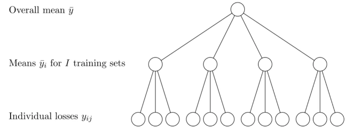
Overall mean ¯y

Means ¯yi forI training sets

Individual losses yij

Figure 2.1: Schematic diagram of the hierarchical design. In this case there are I = 4 disjoint

training sets and I= 4 disjoint test sets each containingJ = 3 cases. Since both training and test

sets are disjoint, the average losses for each training set ¯yiare independent estimates of the expected

lossµ.

using these designs. It is possible that there is some way of overcoming the difficulties and this would certainly be of importance if one hopes to be able to use small datasets for benchmarking. It should be noted that when n-way cross-testing is usually used in the literature, one does not attempt to estimate uncertainties associated with the performance estimates. In such cases it is not easy to justify the conclusions of the experiments.

2.4 Hierarchical ANOVA design

The simplest loss model that we will consider is the analysis of variance (ANOVA) in the hierarchical design. In this loss model, the learning algorithm is trained on I different training sets. These training sets are disjoint, i.e., a specific training case appears only in a single training set. Associated with each of the training sets there is a test set withJ cases. These test sets are also disjoint from one another and disjoint from the training sets. We train the method on each of theI training sets and for each training set we evaluate the loss on each case in the corresponding test set. A particular training set and the associated test cases will be referred to as an instance of the task in the following. We assume that the losses can be modeled by

yij =µ+ai+εij. (2.2)

(21)

2.4 Hierarchical ANOVA design 15

set i. The ai and εij are assumed Normally and independently distributed with

ai∼ N(0, σa2) εij ∼ N(0, σe2). (2.3) Theµ parameter models the mean loss which we are interested in estimating. Theai vari-ables are called the effects due to training set, and can model the variability in the losses that is caused by varying the training set. Note, that the training set effects include all sources of variability between the different training sessions: the different training examples and stochastic effects in training, e.g., random initialisations. Theεij variables model the residuals; these include the effects of the test cases, interactions between training and test cases and stochastic elements in the prediction procedure. For some loss functions, these Normality assumptions may not seem appropriate; refer to section 2.6 for a further discus-sion. In the following analysis, we will not attempt to evaluate the individual contributions to theai and εij effects.

Using eq. (2.2) and (2.3) we can obtain the estimated expected loss and one standard deviation error bars on this estimate

ˆ

µ= ¯y SD(ˆµ) =σ

2 a

I +

σ2 ε

IJ

1/2

, (2.4)

where a hat indicates an estimated value, and a bar indicates an average. This estimated standard error is for fixed values of the σ’s, which we can estimate from the losses. We introduce the following means

¯ yi=

1 J

X

j

yij y¯=

1 IJ

X

i

X

j

yij, (2.5)

and the “mean squared error” for aand εand their expectations MSa =

J I₋1

X

i

(¯yi−y¯)2 E[MSa] = Jσa2+σε2 MSε =

1 I(J₋1)

X

i

X

j

(yij−y¯i)2 E[MSε] = σ2ε.

(2.6)

In ANOVA models it is common to use the following minimum variance unbiased estimators for theσ2 values which follow directly from eq. (2.6)

ˆ

σ_ε2= MSε σˆa2=

MSa−MSε

J . (2.7)

Unfortunately the estimate ˆσ2

amay sometimes be negative. This behaviour can be explained by referring to fig. 2.1. There are two sources of variation in ¯yi; firstly the variation due to the differences in the training sets used and secondly the uncertainty due to the finitely

(22)

many test cases evaluated for that training set. This second contribution may be much greater than the former, and empirically eq. (2.7) may produce negative estimates if the variation in ¯yi values is less than expected from the variation over test cases. It is customary to truncate negative estimates at zero (although this introduces bias).

In order to compare two learning algorithms the same model can be applied to thedifferences

between the losses from two learning methods kand k′

yij =yijk−yijk′ =µ+a_i+ε_ij, (2.8)

with similar Normal and independence assumptions as before, given in eq. (2.3). In this case µ is the expected difference in performance and ai is the training set effect on the difference. Similarly,εij are residuals for the difference loss model. It should be noted that the tests derived from this model are known aspaired tests, since the losses have been paired according to training sets and test cases. Generally paired tests are more powerful than non-paired tests, since random variation which is irrelevant to the difference in performance is filtered out. Pairing requires that the same training and test sets are used for every method. Pairing is readily achieved in DELVE, since losses for methods are kept on disk. A central objective in a comparative loss study is to get a measure of how confident we can be that the observed difference between the two methods reflects a real difference in performance rather than a random fluctuation. Two different approaches will be outlined to this problem: the standard t-test and a Bayesian analysis.

The idea underlying the t-test is to assume anull hypothesis, and compute how probable the observed data or more extreme data is under the sampling distribution given the hypothesis. In the current application, the null hypothesis is H0: µ = 0, that the two models have identical average performances. It may seem odd to focus on this null hypothesis, when it would seem more natural to draw our conclusions based on p(µ <0_|{yij}) and p(µ > 0|{yij}). The reasoning underlying the frequentist test of H0 is the following: if we can show that we are unlikely to get the observed losses given the null hypothesis, then we can presumably have confidence in the sign of the difference. Technically, the treatment of composite hypothesis, such asH′

0:µ <0 is much more complicated than a simple hypothesis. Thus, since H0 can be treated as a simple hypothesis (through exact analytical treatment of the unknown σ_a2 and σ_ε2), this is often preferred although it may at first sight seem less appropriate.

(23)

partial means can be obtained from eq. (2.8), giving

yij ∼ N(0, σ2a+σε2), y¯i ∼ N(0, σ2a+σ2ε/J) (2.9) for which the variances are unknown in a practical application. The different partial means ¯

yi are independent observations from the above Gaussian distribution. A standard result (dating back to Student and Fisher) from the theory of sampling distributions states if ¯yi is independently and Normally distributed with unknown variance, then the t-statistic

t= ¯y 1

I(I−1)

X

i

(¯yi−y¯)2

−₁_/₂

(2.10) has a sampling distribution given by the t-distribution withI₋1 degrees of freedom

p(t)∝1 + t 2 I−1

−_I/₂

. (2.11)

To perform a t-test, we compute the t-statistic, and measure how unlikely it would be (under the null hypothesis) to obtain the observed t-value or something more extreme. More precisely, the p-value is

p= 1−

Z t −_t

p(t′

)dt′

, (2.12)

for which there does not exist a closed form expression; numerically it is easily evaluated via the incomplete beta distribution for which rapidly converging continued fractions are known, [Abramowitz and Stegun 1964]. Notice, that the t-test is two-sided, i.e., that the limits of the integral are±t, reflecting our prior uncertainty as to which method is actually the better. If in contrast it was apriori inconceivable that the true value ofµwas negative we could use a one-sided test, extending the integral to −∞ and getting a p-value which was only half as large.

Very low p-values thus indicate that we can have confidence that the observed difference is not due to chance. Notice that failure to obtain small p-values does not necessarily imply that the performance of the methods are equal, but merely that the observed data does not rule out this possibility, or the possibility that the sign of the actual difference differs from that of the observed difference.

Fig. 2.2 shows an example of the output from DELVE when comparing two methods. Here the estimates of performances ¯yk and ¯yk′, their estimated difference ˆµ and the standard

error on this estimate SD(ˆµ) are given and below the two effects ˆσa and ˆσε. Finally, the p-value for a t-test is given for the significance of the observed difference.

At this point it may be useful to note that the standard error for the difference estimate SD(ˆµ) is computed using fixed estimates for the standard deviations, given by eq. (2.7),

(24)

Estimated expected loss for knn-cv-1: 357.909 Estimated expected loss for /lin-1: 397.82 Estimated expected difference: -39.9114 Standard error for difference estimate: 11.4546 SD from training sets and stochastic training: 15.3883 SD from test cases & stoch. pred. & interactions: 271.541

Significance of difference (T-test), p = 0.0399302

Based on 4 disjoint training sets, each containing 256 cases and 4 disjoint test sets, each containing 256 cases.

Figure 2.2: An example of applying this analysis to comparison of the two methods lin-1and knn-cv-1using the squared error loss function on the taskdemo/age/std.256in DELVE.

where the distribution of ˆµ is Gaussian. However, there is also uncertainty associated with the estimates for these standard deviations. This could potentially be used to obtain better estimates of the standard error for the difference (interpreted as a 68% confidence interval); computationally this may be cumbersome, since it requires evaluations oftfromp in eq. (2.12) which is a little less convenient. For reasonably large values ofI the differences will be small, and our primary interest is not in these intervals but rather in the p-values (which are computed correctly).

As an alternative to the frequentist hypothesis test, one can adopt a Bayesian viewpoint and attempt to compute the posterior distribution ofµfrom the observed data and a prior distribution. In the Bayesian setting the unknown parameters are the mean difference µ and the two variancesσ2_a and σ_ε2. Following Box and Tiao [1992] the likelihood is given by

p({yij}|µ, σa2, σ2ε)∝ (σ2_ε)−_I₍_J−₁₎_/₂

(σ2_ε+Jσ_a2)−_I/₂

exp₋J

P

i(¯yi−µ)2 2(σ2

ε+Jσ2a) −

P

i

P

j(yij−y¯i)2 2σ2

ε

.

(2.13)

We obtain the posterior distribution by multiplying the likelihood by a prior. It may not in general be easy to specify suitable priors for the three parameters. In such circumstances it is sometimes possible to dodge the need to specify subjective priors by using improper informative priors. The simplest choices for improper priors are the standard non-informative

p(µ)_∝1 p(σ_a2)_∝σ−₂

a p(σ2ε)∝σ

−₂

ε , (2.14)

since the variances are positive scale parameters. In many cases the resulting posterior is still proper, despite the use of these priors. However, in the present setting these priors do not lead to proper posteriors, since there is a singularity atσ2_a= 0; the data can be explained (i.e., acquire non-vanishing likelihood) by the σ2

(25)

will approach infinity as σ2_a goes to zero. This inability to use a non-informative improper prior reflects a real uncertainty in the analysis of the design. For small values of σ2_a the likelihood is almost independent of this parameter and the amount of mass placed in this region of the posterior is largely determined by the prior. In other words, the likelihood does not provide much information aboutσ2

ain this region. An alternative prior is proposed in Box and Tiao [1992], setting

p(µ)∝1 p(σ2_ε)∝σ−2

ε p(σε2+Jσ2a)∝(σε2+Jσ2a)

−1

. (2.15)

This prior has the somewhat unsatisfactory property that the effective prior distribution depends on J, the number of test cases per training set, which is an unrelated arbitrary choice by the experimenter. On the positive side, the simple form of the posterior allows us to express the marginal posterior forµ in closed form

p(µ_|{yij}) =

Z ∞

0

Z ∞

0

p(µ, σ_ε2, σ2_a)p(_{yij}|µ, σ2a, σε2)dσ2adσε2

∝a−p2

2 betaia2/(a1+a2)(p2, p1),

(2.16)

where betai is the incomplete beta distribution and a1 =

1 2

X

i

X

j

(yij−y¯i)2 a2= J

2

X

i

(¯yi−µ)2 p1 =

I(J ₋1)

2 p2 =

I

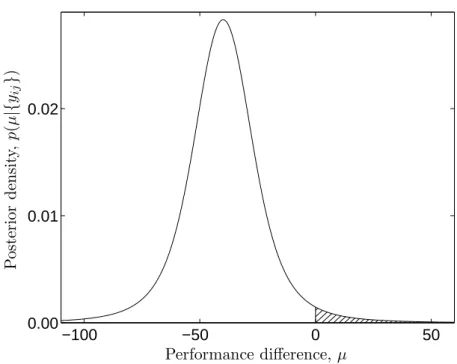
2. (2.17) In fig. 2.3 the posterior distribution ofµ is shown for a comparison between two learning methods. The p-value from the frequentist test in fig. 2.2 is p= 0.040 which is reasonably close to the posterior probability that µ has the opposite sign of the observed difference, which was calculated by numerical integration to be 2.3%. These two styles of analysis are making statements of a different nature, and there is no reason to suspect that they should produce identical values. Whereas the frequentist test assumes that µ = 0 and makes a statement about the probability of the observed data or something more extreme, the Bayesian analysis treats µas a random variable. However, it is reassuring that they do not differ to a great extent.

There are several reasons that I have not pursued the Bayesian analysis further. The most important reason is that my primary concern was to find a methodology which could be adopted in DELVE, for which the Bayesian method does not seem appropriate. Firstly, because the Bayesian viewpoint is often met with scepticism, and secondly because of analytical problems when attempting to use priors other than eq. (2.15). Perhaps the most promising approach would be to use proper priors and numerical integration to evaluate eq. (2.16) and then investigate how sensitive the conclusions are to a widening of the priors. Sampling approaches to the problem of estimating the posterior may be viable, and open

(26)

−100 −50 0 50

0.00 0.01 0.02

Performance difference, µ

P

os

te

ri

or

d

en

si

ty

,

p

(

µ

|{

yij

}

)

Figure 2.3: Posterior distribution ofµ when comparing thelin-1andknn-cv-1methods on the demo/age/std.256data for squared error loss, using eq. (2.16). By numerical integration it is found

that 2.3% of the mass lies at positive values forµ(indicated by hatched area).

up interesting possibilities of being able to relax some of the distributional assumptions underlying the frequentist t-test. However, extreme care must be taken when attempting to use sampling methods (such as simple Gibbs sampling) where it may be hard to ensure convergence, since this may leave the conclusions from experiments open to criticism.

2.5 The 2-way ANOVA design

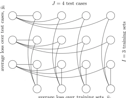
The experimental setup for a 2-way design differs from the hierarchical design in that we use all the test cases for every training session thereby gaining more information about the performances, fig. 2.4. This is more efficient (in terms of data) which may be important if the number of available cases is small. However, the analysis of this model is more complicated. The loss model is:

yij =µ+ai+bj+εij, (2.18)

withai being the effects for the training sets,bj the effects for the test cases, andεij their interactions and noise. As was the case for the hierarchical design, these effects may have several different components, but no attempt will be made to estimate these individually.

(27)

2.5 The 2-way ANOVA design 21

J = 4 test cases

average loss over training sets, ¯yj

av

er

ag

e

lo

ss

ov

er

te

st

ca

se

s,

¯

yi

I

=

3

tr

ai

n

in

g

se

ts

Figure 2.4: Schematic diagram of the 2-way design. There are I = 3 disjoint training sets and a

common test set containingJ= 4 cases giving a total of 12 losses. The partial average performances

are not independent.

We make the same assumptions of independence and normality as previously

ai∼ N(0, σa2) bj ∼ N(0, σb2) εij ∼ N(0, σε2). (2.19) In analogy with the hierarchical design, these assumptions give rise to the following expec-tation and standard error

ˆ

µ= ¯y SD(ˆµ) =σ

2 a

I +

σ_b2

J +

σ_ε2 IJ

1/2

. (2.20)

We introduce the following partial mean losses ¯

y = 1

IJ

X

i

X

j

yij y¯i= 1 J

X

j

yij y¯j = 1 I

X

i

yij, (2.21)

and the “mean squared error” for a,b and εand their expectations: MSa=

J I−1

X

i

(¯yi−y¯)2 E[MSa] =Jσa2+σε2

MSb =

I J₋1

X

j

(¯yj−y¯)2 E[MSb] =Iσb2+σε2

MSε=

1 (I₋1)(J ₋1)

X

i

X

j

(yij−y¯)−(¯yi−y¯)−(¯yj −y¯)

2

E[MSε] =σ2ε (2.22) Now we can use the empirical values of MSa, MSb and MSε to estimate values for the σ’s:

ˆ

σε2 = MSε σˆb2 =

MSb−MSε

I σˆa

2 ₌ MSa−MSε

(28)

These estimators are uniform minimum variance unbiased estimators. As before, the esti-mates for σ_a2 and σ_b2 are not guaranteed to be positive, so we set them to zero if they are negative. We can then substitute these variance estimates into eq. (2.20) to get an estimate for the standard error for the estimated mean performance.

Note that the estimated standard error ˆσdiverges if we only have a single training set (as is common practice!). This effect is caused by the hopeless task of estimating an uncertainty from a single observation. At least two training sets must be used and probably more if accurate estimates of uncertainty are to be achieved.

Another important question is whether the observed difference between two learning pro-cedures can be shown to be significantly different from each other. To settle this question we again use the model from eq. (2.18), only this time we model the difference between the losses of the two models,k andk′

:

yijk−yijk′ =µ+a_i+b_j+ε_ij, (2.24)

under the same assumptions as above. The question now is whether the estimated overall mean difference ˆµ is significantly different from zero. We can test this hypothesis using a quasi-F test [Lindman 1992], which uses the F statistic with degrees of freedom:

Fν1,ν2 = (SSm+ MSε)/(MSa+ MSb), where SSm =IJy¯

2

ν1 = (SSm+ MSε)2/(SS2m+ MS2ε/((I−1)(J −1))) (2.25)

ν2 = (MSa+ MSb)2/(MS2a/(I−1) + MS2b/(J−1)).

The result of the F-test is a p-value, which is the probability given the null-hypothesis (µ = 0) is true, that we would get the observed data or something more extreme. In general, low p-values indicates a high confidence in the difference between the performance of the learning procedures.

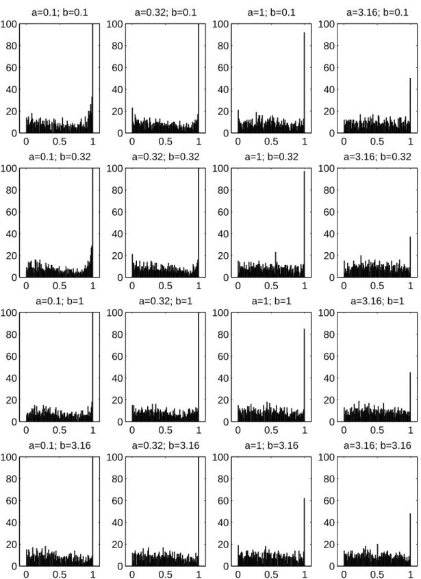
Unfortunately this quasi-F test is only approximate even if the assumptions of independence and Normality are met. I have conducted a set of experiments to clarify how accurate the test may be. For our purposes, the most serious mistake that can be made is what is nor-mally termed a type I error: concluding that the performances of two methods are different when in reality they are not. In our experiments, we would not normally anticipate that the performance of two different methods would be exactly the same, but if we ensure that the test only rarely strongly rejects the null hypothesis if it is really true, then presumably it will be even rarer for it to declare the observed difference significant if its sign is opposite to that of the true difference.

(29)

2.5 The 2-way ANOVA design 23

0 0.5 1 0 20 40 60 80 100 a=0.1; b=0.1

0 0.5 1 0 20 40 60 80 100 a=0.32; b=0.1

0 0.5 1 0 20 40 60 80 100 a=1; b=0.1

0 0.5 1 0 20 40 60 80 100 a=3.16; b=0.1

0 0.5 1 0 20 40 60 80 100 a=0.1; b=0.32

0 0.5 1 0 20 40 60 80 100 a=0.32; b=0.32

0 0.5 1 0 20 40 60 80 100 a=1; b=0.32

0 0.5 1 0 20 40 60 80 100 a=3.16; b=0.32

0 0.5 1 0 20 40 60 80 100 a=0.1; b=1

0 0.5 1 0 20 40 60 80 100 a=0.32; b=1

0 0.5 1 0 20 40 60 80 100 a=1; b=1

0 0.5 1 0 20 40 60 80 100 a=3.16; b=1

0 0.5 1 0 20 40 60 80 100 a=0.1; b=3.16

0 0.5 1 0 20 40 60 80 100 a=0.32; b=3.16

0 0.5 1 0 20 40 60 80 100 a=1; b=3.16

0 0.5 1 0 20 40 60 80 100 a=3.16; b=3.16

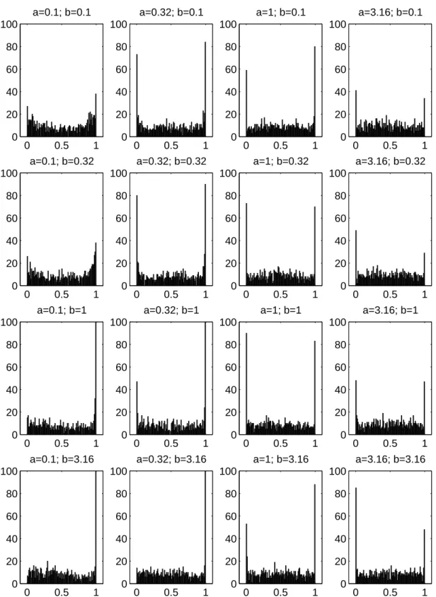
Figure 2.5: Experiments using 2 training instances, showing the empirical distribution of 1000

p-values in 100 bins obtained from fake observations from under the null hypothesis. Hereaand b

(30)

0 0.5 1 0 20 40 60 80 100 a=0.1; b=0.1

0 0.5 1 0 20 40 60 80 100 a=0.32; b=0.1

0 0.5 1 0 20 40 60 80 100 a=1; b=0.1

0 0.5 1 0 20 40 60 80 100 a=3.16; b=0.1

0 0.5 1 0 20 40 60 80 100 a=0.1; b=0.32

0 0.5 1 0 20 40 60 80 100 a=0.32; b=0.32

0 0.5 1 0 20 40 60 80 100 a=1; b=0.32

0 0.5 1 0 20 40 60 80 100 a=3.16; b=0.32

0 0.5 1 0 20 40 60 80 100 a=0.1; b=1

0 0.5 1 0 20 40 60 80 100 a=0.32; b=1

0 0.5 1 0 20 40 60 80 100 a=1; b=1

0 0.5 1 0 20 40 60 80 100 a=3.16; b=1

0 0.5 1 0 20 40 60 80 100 a=0.1; b=3.16

0 0.5 1 0 20 40 60 80 100 a=0.32; b=3.16

0 0.5 1 0 20 40 60 80 100 a=1; b=3.16

0 0.5 1 0 20 40 60 80 100 a=3.16; b=3.16

Figure 2.6: Experiments using 4 training instances, showing the empirical distribution of p-values

obtained from fake observations from under the null hypothesis. Here a and b give the standard

(31)

2.6 Discussion 25

I generated mock random losses under the null hypothesis, from eq. (2.18) and (2.19) with µ≡0 andσε= 1.0 for various values ofσa andσb. The unitσεsimply sets the overall scale without loss of generality. I then computed the p-value for the F-test for repeated trials. In fig. 2.5 and 2.6 are histograms of the resulting p-values. Ideally these histograms ought to show a uniform distribution — the reason why these do not (apart from finite sample effects) is due to the approximation in the F-test. The most prominent effects are the spikes in the histograms around p = 0 and p = 1. The spikes at p = 1 are not of great concern since the test here is strongly in favor of the (true) null hypothesis. This may lead to a reduced power of the test, but not to type I errors. The spikes that occur around p = 0 are directly of concern. Here the test is strongly rejecting the null hypothesis, leading us to infer that the methods have differing performance when in fact they do not. This effect is only strong in the case where there are only 2 instances and where the training set effect is large. With 4 instances (and 8, not shown) these problems have more or less vanished. To avoid interpretative mistakes whenever there are fewer than 4 instances and the computed p-value is less than 0.05, the result is reported by DELVE as p <0.05.

2.6 Discussion

One may wonder what happens to the tests described in earlier sections when the assump-tions upon which they rely are violated. The independence assumpassump-tions should be fairly safe, since we are carefully designing the training and test sets with independence in mind. The Normality assumptions however, may not be met very well. For example, it is well known that when using squared error loss, one often sees a few outliers accounting for a large fraction of the total loss over the test set. In such cases one may wonder whether squared error loss is really the most interesting loss measure. Given that we insist on pursuing this loss function, we need to consider violations of Normality.

The Normality assumptions of the experimental designs are obviously violated in the case of loss estimation for squared error loss functions, which are guaranteed positive. This ob-jection disappears for the comparative designs where only the loss differences are assumed Normal. However, it is well known that extreme losses may occour — so Gaussian assump-tions may be inappropriate. As a solution to this problem, Prechelt [1994] suggests using the log of the losses in t-tests after removing up to 10% “outliers”. I do not advocate this approach. The loss function should reflect the function that one is interested in minimising. If one isn’t concerned by outliers then one should choose a loss function that reflects this. Removing outlying losses does not appear defensible in a general application. Also, method

(32)

A having a smaller expected log loss than method B does not imply anything about the relation of their expected losses.

Generally, both the t-test and F-test are said to be fairly robust to small deviations from Normality. Large deviations in the form of huge losses from occasional outliers turn out to have interesting effects. For the comparative loss models described in the previous sections, the central figure determining the significance of an observed difference is the ratio of the mean difference to the uncertainty in this estimate ¯y/σˆ, as in eq. (2.10). If this ratio is large, we can be confident that the observed difference in not due to chance. Now, imagine a situation where ¯y/σˆ is fairly large; we select a loss difference y′

at random and perturb it by an amountξ, and observe the behaviour of the ratio as we increaseξ

¯ y ˆ

σ =

P

yi+ξ

q

n(P

y2

i +ξ2+y′ξ)−(

P

yi+ξ)2

→ √ 1

n−1 when ξ → ∞. (2.26) Thus, for large values ofnthe tests will tend to become less significant, as the magnitude of the outliers increase. Here we seem to be lucky that outliers will not tend to produce results that appear significant but merely reduce the power of the test. However, this tendency may in some cases have worrying proportions. In fact, let’s say we are testing two methods against each other, and one seems to be doing significantly better than the other. Then the losing method can avoid losing face in terms of significance by increasing its loss on a single test case drastically. Because the impact on the mean is smaller than the impact on ˆ

σ for such behaviour, the end result for large ξ is a slightly worse performance for the bad method, but insignificant test results. This scenario is not contrived; I have seen its effects on many occasions and we shall see it in Chapter 5.

This somewhat unsatisfactory behaviour arises from the symmetry assumptions in the loss model. If the losses for one model can have occasional huge values, and the distribution of loss differences is assumed symmetric, it could also happen (although it didn’t) that the other model would have a huge loss, hence the insignificant result. Clearly, this is not exactly what we had in mind. There may be cases where these assumptions are reasonable, but there are situations where some methods may tend to make wild predictions while others are more conservative.

It is possible that these deficiencies could be overcome in a Bayesian setting that allowed for non-Gaussian and skew distributional assumptions. It seems obvious that great care must be taken when designing such a scheme, both with respect to its theoretical properties as well as provisions for a satisfactory implementation of the required computations.

(33)

2.6 Discussion 27

Another idea as to how this situation could be remedied is to allow the “winning” method to perturb the losses of the “losing” method, subject to the constraint that losses of the losing method may only be lowered. This may in many cases alleviate the problems of insignificance in situations plagued by extreme losses in a competing method. Several questions remain open in respect to this approach. What is the sampling distribution for the obtained p-values under the null hypothesis? Is there a unique (and simple) way of figuring out which losses to perturb and by how much? I have not pursued these ideas further, but this may well be worthwhile. For the time being, it underlines that one should always consider both the mean difference in performance as well as the p-value for the test. This will also help reduce the importance of very small p-values when they are associated with negligible reductions in loss.

The loss models considered in this chapter have mainly been developed with continuous loss functions in mind. Continuous loss functions are used when the outputs are continuous, and tasks of classification can similarly be handled if one has access to the output class probabilities (which are continuous). However, it is also quite common to use the binary 0/1-loss function for classification. It is not quite obvious how well the present loss models will work for binary losses. Clearly, the assumptions about Normality are not appropriate — but they will probably not lead to ridiculous conclusions. It does not seem straightforward to design more appropriate models for discrete losses that allow for the necessary components of variability. An empirical study of tests of difference in performance of learning methods for binary classification has appeared in [Dietterich 1996].

(34)

(35)

Chapter 3

Learning Methods

3.1 Algorithms, heuristics and methods

A prerequisite of measuring the performance of a learning method is defining exactly what the method is. This may seem like a trivial statement, but a detailed investigation reveals that it is uncommon in the neural network literature to find a description of an algorithm that is detailed enough to allow replication of the experiments — see [Quinlan 1993; Thod-berg 1996] for examples of unusually detailed descriptions. For example, an article may propose to use part of the training data for a neural network as a validation set to mon-itor performance while training and to stop training when a minimum in validation error is encountered (this is known as early stopping). I will refer to such a description as an

algorithm. This algorithm must be accompanied by details of the implementation, which I will call heuristics in order to produce a method which is applicable to practical learn-ing problems. In this example, the heuristics would include details such as the network architecture, the minimization procedure, the size of the validation set, rules for how to determine whether a minimum in validation error was reached, etc.

It is often appealing to think of performance comparisons in terms of algorithms and not heuristics. For example, one may wish to make statements like: “Linear models are su-perior to neural networks on data from this domain”. In this case we are clearly talking about algorithms, but as I have argued above, the empirical assessments supporting such statements necessarily involve the methods — including heuristics. We hope that in most cases the exact details of the heuristics are not crucial to the performance of the method, so

(36)

30 Learning Methods

that it will be reasonable to generalise the results of the methods to the algorithm itself. It should be stressed that the experimental results involving methods are the objective basis of the more subjective (but more useful) generalisations about algorithms. A more principled approach of investigating several sets of heuristics for each algorithm would be extremely arduous and would still not address the central issue of attempting to project experimental results to novel applications.

I focus my attention on automatic methods, i.e., methods that can be applied without human intervention. The reason for this choice is primarily a concern about reproducibility. It may be argued that for practical problems one should allow a human expert to design special models that take the particular characteristics of the learning problem into account. This does not rule out the usefulness of automatic procedures as aids to an expert. Also, it may be possible to invent heuristics which embody some of the “common sense” of the expert — however, it turns out that this can be an extremely difficult endeavor. My approach is to try to develop methods with sufficiently elaborate heuristics that the method cannot be improved upon by a simple (well documented) modification. I require the methods to be automatic, but I monitor the progress of the algorithm and take note of the cases where the heuristics seem to break down, in order to be able to identify the reasons for poor performance.

The primary target of comparisons is the predictive performance of the methods. However, it does not seem reasonable to completely ignore computational issues, such as cpu time and memory requirements. For many algorithms one may expect there to be a tradeoff between predictive accuracy and cpu time — for example when training an ensemble of networks, we may expect the performance to improve as the ensemble gets larger. I wish to study algorithms that have a reasonably large amount of cpu time at their disposal. For many practical learning problems a few days of cpu time on a fast computer would typically not seem excessive. However, for practical reasons I will limit the computational resources to a few hours per task.

It turns out that it is convenient from a practical point of view to develop heuristics for a particular amount of cpu time, so that the algorithm itself can make choices based on the amount of time spent so far, etc. As an example, consider the case of training an ensemble of 10 networks. In general, reasonable heuristics for this problem are difficult to devise because it may be very hard to determine how long it is necessary to train the individual nets for. If we have a fixed time to run the algorithm, we may circumvent this problem by simply training all nets for an equal amount of time. Naturally, it may turn out that none of the nets were trained well in this time; indeed, it may turn out to have been better to

(37)

3.2 The choice of methods 31

train a single net for the entire allowed period of time, instead of trying an ensemble of 10 nets. I have used this convenient notion of a cpu time constraint for many of the methods, although this may not correspond well to realistic applications. In the experiments, the algorithms will be tested for different amounts of allowed time, and from these performance measures it is usually possible to judge whether the algorithm could perform better given more time.

3.2 The choice of methods

In this thesis, experiments are carried out using eight different methods. Six of these methods will be described in the remainder of this chapter and the two methods relying on Gaussian processes will be developed in the following chapter.

Two of the methods, a linear method called lin-1 and a nearest neighbor method using cross-validation to choose the neighborhood size calledknn-cv-1, rely on simple ideas that are often used for data modeling. These methods are included as a “base-line” of per-formance, to give a feel for how well simple methods can be expected to perform on the tasks.

Two versions of the MARS (Multivariate Regression Splines) method have been included. This method was developed by Friedman [1991], who has also supplied the software. This method is not described in detail in this thesis, since it has been published by Friedman. The primary goal of including these methods is to provide some insight into how neural network methods compare to methods developed in the statistics community with similar aims.

Themlp-ese-1method relies on ensembles of neural networks trained with early stopping. This method is included as an attempt at a thorough implementation of the commonly used early stopping paradigm. The intention of including this method is to get an impression of the accuracy that can be expected from this widely-used technique.

The mlp-mc-1method implements Bayesian learning in neural networks. The software for this method was developed by Neal [1996]. This method uses Monte Carlo techniques to fit the model and may be fairly computer intensive. Given enough time, one may expect this method to have very good predictive performance. It should thus be a strong competitor.