How Boosting the Margin Can Also Boost Classifier Complexity

(1)

Yale University, Department of Computer Science, 51 Prospect Street, New Haven, CT 06520, USA

Princeton University, Department of Computer Science, 35 Olden Street, Princeton, NJ 08540, USA

Abstract

Boosting methods are known not to usu-ally overfit training data even as the size of the generated classifiers becomes large. Schapire et al. attempted to explain this phe-nomenon in terms of the margins the clas-sifier achieves on training examples. Later, however, Breiman cast serious doubt on this explanation by introducing a boosting algo-rithm, arc-gv, that can generate a higher margins distribution than AdaBoost and yet

performs worse. In this paper, we take a

close look at Breiman’s compelling but puz-zling results. Although we can reproduce his main finding, we find that the poorer per-formance of arc-gv can be explained by the increased complexity of the base classifiers it uses, an explanation supported by our exper-iments and entirely consistent with the mar-gins theory. Thus, we find maximizing the margins is desirable, but not necessarily at the expense of other factors, especially base-classifier complexity.

1. Introduction

The AdaBoost boosting algorithm (Freund &

Schapire, 1997) and most of its relatives produce clas-sifiers that classify by voting the weighted predictions of a set of base classifiers which are generated in a se-ries of rounds. Thus, the size — and hence, naively, the apparent complexity — of the final combined clas-sifier used by such algorithms increases with each new round of boosting. Therefore, according to Occam’s razor (Blumer et al., 1987), the principle that less com-plex classifiers should perform better, boosting should

Appearing in Proceedings of the 23rd International Con-ference on Machine Learning, Pittsburgh, PA, 2006. Copy-right 2006 by the author(s)/owner(s).

suffer from overfitting; that is, with many rounds of boosting, the test error should increase as the final

classifier becomes overly complex. Nevertheless, it

has been observed by various authors (Breiman, 1998; Drucker & Cortes, 1996; Quinlan, 1996) that boosting often tends to be resistant to this kind of overfitting, apparently in defiance of Occam’s razor. That is, the test error of AdaBoost often tends to decrease well af-ter the training error is zero, and does not increase

even after a very large number of rounds.1

Schapire et al. (1998) attempted to explain AdaBoost’s tendency not to overfit in terms of the margins of the

training examples, where themarginis a quantity that

can be interpreted as measuring the confidence in the prediction of the combined classifier. Giving both the-oretical and empirical evidence, they argued that with more rounds of boosting, AdaBoost is able to increase the margins, and hence the confidence, in the predic-tions that are made on the training examples, and that this increase in confidence translates into better per-formance on test data, even if the boosting algorithm is run for many rounds.

Although Schapire et al. backed up their arguments with both theory and experiments, Breiman (1999) soon thereafter presented experiments that raised im-portant questions about the margins explanation. Fol-lowing the logic of the margins theory, Breiman at-tempted to design a better boosting algorithm, called arc-gv, that would provably maximize the minimum margin of any training example. He then ran experi-ments comparing the performance of arc-gv and Ada-Boost using CART decision trees pruned to a fixed number of nodes as base classifiers. He found that arc-gv did indeed produce uniformly higher margins than AdaBoost. However, contrary to what was apparently predicted by the margins theory, he found that his new

1

However, in some of these cases, the test error has been observed to increase slightly after anextremelylarge number of rounds (Grove & Schuurmans, 1998).

(2)

algorithm arc-gv performed worse on test data than AdaBoost in almost every case. Breiman concluded rather convincingly that his experiments put the mar-gins explanation into serious doubt and that a new understanding is needed.

In this paper, we take a close look at these compelling experiments to try to determine if they do in fact con-tradict the margins theory. In fact, the theory that was presented by Schapire et al. states that the gen-eralization error of the final combined classifier can be upper bounded by a function that depends not only on the margins of the training examples, but also on the number of training examples and the complexity of the base classifiers (where complexity might, for in-stance, be measured by VC-dimension or description length). Breiman was well aware of this dependence on the complexity of the base classifiers and attempted to control for this factor in his experiments by always choosing decision trees of a fixed size. However, in our experiments, we find that there still remain important differences between the trees chosen by AdaBoost and arc-gv. Specifically, we find that the trees produced using arc-gv are considerably deeper, both in terms of maximum and average depth of the leaves. Intuitively, such deep trees are more prone to overfitting, and in-deed, it is clear that the space of decision trees of a given size is much more greatly constrained when a bound is placed on the depth of the leaves. Further-more, we find experimentally that the deeper trees gen-erated by arc-gv are measurably more prone to over-fitting than those of AdaBoost. The use of depth as a measure of tree complexity was also suggested in the work of Mason, Bartlett and Golea (2002) who worked on finding more refined ways of measuring the complexity of a decision tree besides its overall size. Thus, we argue that the trees found by arc-gv have topologies that are more complex in terms of their ten-dency to lead to overfitting, and that this increase in complexity accounts for arc-gv’s inferior performance on test data, an argument that is consistent with the margins theory.

We then consider the use of other base classifiers, such as decision stumps, whose complexity can be more tightly controlled. We again compare the performance of AdaBoost and arc-gv, and again find that Ada-Boost is superior, despite the fact that base classi-fiers of equivalent complexity are being used, and de-spite the fact that arc-gv tends to obtain a higher minimum margin than AdaBoost. Nevertheless, on close inspection, we see that the bounds presented by

Schapire et al. are in terms of the entire distribution

of margins, not just theminimum margin. When this

overall margin distribution is examined, we find that although arc-gv obtains a higher minimum margin, the margin distribution as a whole is very much higher for AdaBoost. Thus, again, these experiments do not ap-pear to contradict the margins theory.

In sum, our experiments explore the complex interplay between margins, base classifier complexity and sam-ple size that helps to determine how well a classifier performs. We believe that understanding this interac-tion better might help us to design better algorithms. In a sense, our results confirm Breiman’s point that maximizing margins is not enough; we also need to think about the other factors, especially base classi-fier complexity, and how that can be driven up by an over-aggressive attempt to increase the margins. Our results also explore the interplay between minimum margin and the overall margins distribution as seen in the way that arc-gv only increases the minimum mar-gin, but AdaBoost sometimes seems to do a better job with the overall distribution.

Our paper focuses only on Breiman’s arc-gv algo-rithm for maximizing margins although others have

been proposed, for instance, by R¨atsch and

War-muth (2002), Grove and Schuurmans (1998) and Rudin, Schapire and Daubechies (2004). Moreover, Mason, Bartlett and Golea (2004) were able to show how the direct optimization of margins could indeed lead to improved performance. We also focus only on the theoretical bounds of Schapire et al., although these have been greatly improved, for instance, by

Koltchinskii and Panchenko (2002). Overviews on

boosting are given by Schapire (2002) and Meir and

R¨atsch (2003).

After reviewing the margins theory in Section 2, we be-gin our study in Section 3 with experiments intended to replicate those of Breiman. In Section 4, we then present evidence that arc-gv produces higher margins by using more complex base classifiers and that its poorer performance is consistent with the margins the-ory. In Section 5, we try to control the complexity of the base classifiers but find that this prevents arc-gv from having a uniformly higher margins distribution.

2. Algorithms and Theory

Boosting algorithms combine moderately inaccurate prediction rules and take their weighted majority vote to form a single classifier. On each round, a boost-ing algorithm generates a new prediction rule to use and then places more weight on the examples classi-fied incorrectly. Hence, boosting constantly focuses on classifying correctly the examples that are the hardest

(3)

Given: (x1, y1), . . . ,(xm, ym)

wherexi∈X,yi∈Y ={−1,+1}

InitializeD1(i) = 1/m.

Fort= 1, . . . , T:

• Train base learner using distributionDt.

• Get base classifierht:X → {−1,+1}.

• Chooseαt∈R.

• Update:

Dt+1(i) =

Dt(i) exp(−αtyiht(xi))

Zt

whereZtis a normalization factor (chosen so that

Dt+1 will be a distribution).

Output the final classifier:

H(x) = sign

T X

t=1

αtht(x) !

Figure 1.A generic algorithm equivalent to both AdaBoost and arc-gv, depending on howαt is selected.

to classify.

Figure 1 presents a generic algorithm that is equivalent to both AdaBoost and arc-gv, depending on the choice

ofαt. Specifically, AdaBoost setsαto be

αt=

1

2ln

1 +γt

1−γt

whereγtis the so-called edgeofht:

γt= X

i

Dt(i)yiht(xi)

which is linearly related toht’s weighted error.

AdaBoost greedily minimizes a bound on the training error of the final classifier. In particular, as shown by Schapire and Singer (1999), its training error is

bounded by Q

tZt, so, on each round, it chooses ht

and setsαto minimizeZt, the normalizing factor.

Freund and Schapire (1997) derived an early bound on the generalization error of boosting, showing that

Pr [H(x)6=y]≤Pr[ˆ H(x)6=y] + ˜O

r

T d m

!

where Pr [·] denotes probability over the distribution

that was assumed to have generated the training

ex-amples, ˆPr[·] denotes the empirical probability on the

training sample, and d is the VC-dimension of the

space of all possible base classifiers. However, this bound becomes very weak as the number of rounds

T increases, and predicts that AdaBoost will quickly

overfit with only a moderate number of rounds. Early experiments (Breiman, 1998; Drucker & Cortes, 1996; Quinlan, 1996), however, showed just the opposite, namely, that AdaBoost tends not to overfit.

Schapire et al.(1998) attempted to explain why boost-ing often does not overfit usboost-ing the concept of mar-gins on the training examples. The margin of example

(x, y) depends on the votes ht(x) with weights αt of

all the hypotheses:

margin(x, y) =y

P

tαtht(x) P

tαt

.

The magnitude of the margin represents the strength of agreement of the base classifiers, and its sign indi-cates whether the combined vote produces a correct prediction. Using the margins, Schapire et al. proved a bound not dependent on the number of boosting

rounds. They showed that for anyθ, the generalization

error is at most ˆ

Pr[margin(x, y)≤θ] + ˜O

r

d mθ2

!

. (1)

We can notice that this margins bound depends most heavily on the margins near the bottom of the distri-bution, since having generally high smallest margins

allowsθ to be small without ˆPr[margin(x, y)≤θ]

get-ting too large.

Following this logic, Breiman (1999) designed arc-gv to greedily maximize the minimum margin. Arc-gv follows the same algorithm as AdaBoost, except for

settingαtdifferently:

αt=

1

2log

1 +γt

1−γt

−1

2log

1 +̺t

1−̺t

where ̺t is the minimum margin over all training

ex-amples of the combined classifier up to the current round:

̺t= min

i yi Pt−1

s=1αshs(xi) Pt−1

s=1αs !

(It is understood that̺1= 0.)

Arc-gv has the property2 _{that its minimum margin}

converges to the largest possible minimum margin,

2

Meir and R¨atsch (2003) claimed they can only prove this property when taking̺tto be the maximum minimum

margin over all previous rounds in the equation above; we nevertheless decided to use Breiman’s original formulation of arc-gv.

(4)

Table 1. Dataset sizes for training and test.

cancer ion ocr 17 ocr 49 splice

training 630 315 1000 1000 1000

test 69 36 5000 5000 2175

provided that the edges are sufficiently large, as will be the case if the base classifier with largest edge is se-lected on every round. Thus, the margin theory would appear to predict that arc-gv’s performance should be better than AdaBoost’s, although as we here explore, there are other factors at play.

3. Breiman’s Experiments

Breiman (1999) showed that it is possible for arc-gv to produce a higher margins distribution and yet

per-form worse. He ran AdaBoost and arc-gv for 100

rounds using pruned CART decision trees as base clas-sifiers. Each such tree was created by generating the full CART tree and pruning it to the best (i.e.,

min-imum weighted error) k-leaf subtree. Breiman’s most

compelling results were for trees of sizek= 16 where

he found that the margins distributions are uniformly higher for arc-gv than for AdaBoost.

We begin our study by replicating his results. How-ever, unlike Breiman, we did not see the margins of arc-gv being significantly higher until we ran the al-gorithms for 500 rounds. Since Breiman’s critique of the margins theory is strongest when the difference in the margins distributions is clear, we focus only on the

500-round case withk= 16.

We considered the following datasets: breast cancer, ionosphere, splice, ocr17, and ocr49, all available from the UCI repository. These include the same natural datasets as Breiman, except the sonar dataset, since it only includes 208 data points and thereby produces high variance in experiment. The splice dataset was modified to collapse the two splice categories into one to create binary-labeled data. Also, ocr17 and ocr49 contain randomly chosen subsets of the NIST database of handwritten digits consisting only of the digits 1 and 7, and 4 and 9 (respectively); in addition, the images

have been scaled down to 14×14 pixels, each with

only four intensity levels. Table 1 shows the num-ber of training and test examples used in each. The stark differences in the training and test sizes among the datasets occur because we used the same random splits Breiman used for ionosphere and breast cancer, but the additional datasets we used had many more data points, which allowed us to use larger sets for

0 0.2 0.4 0.6 0.8 1 1.2

0.5 0.6 0.7 0.8 0.9 1

cumulative frequency

margin

"AdaBoost_bc" "Arc-gv_bc"

Figure 2.Cumulative margins for AdaBoost and arc-gv for the breast cancer dataset after 500 rounds of boosting.

Table 2.Test errors, averaged over 10 trials, of AdaBoost and arc-gv, run for 500 rounds using CART decision trees pruned to 16 leaf nodes as base classifiers.

cancer ion ocr 17 ocr 49 splice

AdaBoost 2.46 3.46 0.96 2.04 3.18

arc-gv 3.04 7.69 1.76 2.38 3.45

test data. In running our experiments, we followed Breiman’s technique of choosing an independently ran-dom subset for training data of sizes specified in the table. All experiments were repeated on ten random partitions of the data, and, in most cases, the results were averaged.

Figure 2 shows the cumulative margins distribution af-ter 500 rounds for both AdaBoost and arc-gv on the breast cancer dataset. As observed by Breiman, arc-gv does indeed produce higher margins. These distribu-tions are representative of the margins distribudistribu-tions for the rest of the datasets.

Table 2 shows the test errors for each algorithm. Again, in conformity with Breiman, we see that the test errors of arc-gv are indeed higher than those of AdaBoost.

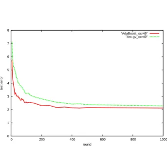
To further visualize what is happening during the run-ning of these algorithms, we plotted both the test error and minimum margin as a function of the number of rounds in Figures 3 and 4. These results seem to be in direct contradiction to the margins theory.

(5)

Table 3.Test errors, minimum margins, and tree depths, averaged over 10 trials, of AdaBoost and arc-gv, run for 500 rounds using CART decision trees pruned to 16 leaf nodes as base classifiers. (For 100 rounds, we also saw arc-gv producing deeper trees on average.)

test error minimum margin tree depth

arc-gv AdaBoost arc-gv AdaBoost arc-gv AdaBoost

breast cancer 3.04 2.46 0.64 0.61 9.71 7.86

ionosphere 7.69 3.46 0.97 0.77 8.89 7.23

ocr 17 1.76 0.96 0.95 0.88 7.47 7.41

ocr 49 2.38 2.04 0.53 0.49 7.39 6.70

splice 3.45 3.18 0.46 0.42 7.12 6.67

0 1 2 3 4 5 6 7 8

0 200 400 600 800 1000

test error

round

"AdaBoost_ocr49" "Arc-gv_ocr49"

Figure 3.Test errors for AdaBoost and arc-gv for the ocr49 dataset as a function of the number of rounds of boosting.

4. Tree Complexity

Can these results be reconciled with the margins ex-planation? In fact, according to Eq. (1), there are factors other than the minimum margin that need to be considered. Specifically, the generalization error of the combined classifier depends both on the margins it generates, the size of the training sample, and on the complexity of the base classifiers. Since the size of the sample is the same for both arc-gv and AdaBoost, after recording the margins, we should examine the complexity of the base classifiers.

How can we measure the complexity of a decision tree? The most obvious measure is the number of leaves in the tree, which, like Breiman, we are already control-ling by always selecting trees with exactly 16 leaves. However, even among all trees of fixed size, we claim that there remain important topological differences that affect the tendency of the trees to overfit. In

0 0.1 0.2 0.3 0.4 0.5 0.6

0 200 400 600 800 1000

minimum margin

round

"AdaBoost_ocr49_margins" "Arc-gv_ocr49_margins"

Figure 4.Minimum margins for AdaBoost and arc-gv for the ocr49 dataset as a function of the number of rounds of boosting.

particular, deeper trees make predictions based on a longer sequence of tests and therefore intuitively tend to be more specialized than shallow trees and thus more likely to overfit.

In fact, arc-gv generates significantly deeper trees than AdaBoost. Table 3 shows the average depths of the trees (measured by the maximum depth of any leaf) in addition to the minimum margin and error rates for each algorithm. We also measured the running aver-age of the tree complexity of both algorithms as the number of rounds increased. The pattern in Figure 5 is representative of the results for most datasets. In this figure, we can see that at the beginning of boost-ing, the depths of the trees generated by AdaBoost converge downward to a value, while the depths of the trees generated by arc-gv continue to increase for about 200 rounds before leveling off to a higher value. It is evident that while arc-gv has higher margins and

(6)

7 7.5 8 8.5 9 9.5 10

50 100 150 200 250 300 350 400 450 500

cumulative average tree depth

round

Figure 5.Cumulative average of decision tree depth for AdaBoost and arc-gv for the breast cancer set for 500 rounds of boosting.

Table 4.Percent test and training errors per generated tree, and their differences, averaged over all CART deci-sion trees generated in 500 rounds of boosting, over 10 trials.

AdaBoost arc-gv

test train diff test train diff

cancer 13.2 9.7 3.5 10.4 6.3 4.1

ion 19.8 10.9 8.9 12.5 2.6 9.9

ocr 17 5.6 3.7 1.9 2.6 0.6 2.0

ocr 49 24.8 21.1 3.7 21.9 17.8 4.1

splice 27.7 23.4 4.3 23.9 19.2 4.7

higher error, it also produces, on average, deeper trees. Referring back to the bound in Eq. (1), we can

up-per bound the VC-dimension d of a finite space of

base classifiers H by lg|H|. Thus, measuring

com-plexity is essentially a matter of counting how many trees there are of bounded depth. Clearly, the more tightly bounded is the depth, the more constrained is the space of allowable trees, and the smaller will

be the complexity measure lg|H|. This can be seen

in Figure 6 which shows the number of 16-leaf tree

topologies of depth at most d, as a function ofd.

So we are claiming that a possible explanation for the better performance of arc-gv despite its higher margins is that it achieves them by choosing from a greater set of base classifiers. By the bound in Eq. (1), we can see that the higher depths of arc-gv trees can be affecting the generalization error even if the margins explanation holds.

0 2e+06 4e+06 6e+06 8e+06 1e+07

2 4 6 8 10 12 14 16

number of trees

max depth

"maxdepth"

Figure 6.The number of tree topologies of depth at most

d, as a function ofd.

In general, we expect the difference between training and test errors to be greater when classifiers are se-lected from a larger or more complex class. Thus, as a further indication that the deeper trees generated by arc-gv are more likely to cause overfitting, we can directly measure the difference between the test error and (unweighted) training error for the trees gener-ated by each algorithm. In Table 4, we can see that this difference is substantially higher for arc-gv than for AdaBoost in each of the datasets. This adds to the evidence that arc-gv is producing higher margins by using trees which are more complex in the sense that

they have a greater tendency to overfit.3

The margins explanation basically says that when all other factors are equal, higher margins result in lower error. Given, however, that arc-gv tends to choose trees from a larger class, its higher test error no longer qualitatively contradicts the margin theory.

5. Controlling Classifier Complexity

Knowing that arc-gv should produce a higher min-imum margin in the limit, and observing that with CART trees, arc-gv produces a uniformly higher dis-tribution than AdaBoost, we wished to fix the com-plexity of the classifiers both algorithms produce. The

3

While it is curious that the test errors of the individ-ual trees generated by arc-gv are on average lower than those for AdaBoost, it does not necessarily follow that the

combination of trees generated by arc-gv should perform better than that produced by AdaBoost. For example, as will be seen in Section 5, decision stumps can work quite well as base classifiers while individually having quite large test and training errors.

(7)

Table 5.Test errors, minimum margins, and average margins averaged over 100 trials, of AdaBoost and arc-gv, run for 100 rounds using decision stumps as weak learners.

test error minimum margin average margin

arc-gv AdaBoost arc-gv AdaBoost arc-gv AdaBoost

cancer 4.15 4.29 -.01 -.06 .07 .27

ionosphere 10.27 9.58 .01 .03 .09 .20

ocr 17 1.12 1.10 .03 .06 .14 .36

ocr 49 6.38 6.28 -.02 -.07 .05 .20

splice 7.22 6.79 -.01 -.07 .06 .21

0 0.2 0.4 0.6 0.8 1 1.2

-0.1 0 0.1 0.2 0.3 0.4 0.5 0.6 0.7

cumulative frequency

margin

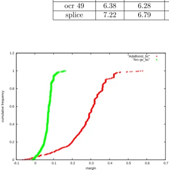
Figure 7.Cumulative margins for AdaBoost and arc-gv for the breast cancer dataset after 100 rounds of boosting on decision stumps.

margins theory tells us that if arc-gv still continued to produce higher margins, it should also perform better. However, if we could see that arc-gv, with some class of weak learners, gets higher margins without gener-ating higher depth trees and still performs worse, it would put the margins theory into serious doubt. A natural class to look at is decision stumps, which are commonly used as base classifiers in boosting and all have the same complexity by most any measure. Yet, looking at sample margins distributions that Ada-Boost and arc-gv generate, in Figure 7, we can see that while arc-gv usually does have a larger minimum margin, it does not have a higher margins distribu-tion overall. In fact, if we look at the average margins, AdaBoost’s are uniformly higher, and once again Ada-Boost on average performs better than arc-gv. These

results are in Table 5.4

4

If arc-gv and AdaBoost run for more rounds, their mar-gins distributions begin to converge, as do their test errors.

Table 6.Percent test and training errors per generated stump, and their differences, averaged over all decision stumps generated in 100 rounds of boosting, over 10 trials.

AdaBoost arc-gv

test train diff test train diff

cancer 40.7 40.5 0.2 41.8 41.7 0.1

ion 42.4 41.4 1.0 42.7 41.8 0.9

ocr 17 34.1 33.9 0.2 34.5 34.2 0.2

ocr 49 42.4 42.0 0.4 43.3 42.9 0.4

splice 42.5 41.9 0.6 43.2 42.7 0.5

This result is both surprising and insightful. We would have expected arc-gv to have uniformly higher margins once more, but this time have lower test error. Yet, it seems that in the case where arc-gv could not pro-duce more complex trees, it sacrificed on the margins distribution as a whole to have an optimal minimum margin in the limit. Knowing this, the margins theory would no longer predict arc-gv to perform better, and it does not.

This is because the margins bound, in Eq. (1), depends

on settingθto be as low as possible while keeping the

probabilityof being less thanθlow. So if the margins of AdaBoost overtake the margins of arc-gv at the lower cumulative frequencies, then the theory would predict AdaBoost to perform better. This is exactly what hap-pens.

For comparison to Table 4, we give in Table 6 the differences between the test and training errors of in-dividual decision stumps generated in 100 rounds of AdaBoost and arc-gv. Consistent with theory, the dif-ferences in these test and training errors for individ-ual stumps are much smaller than they are for CART

Hence, in the few data sets where AdaBoost has slightly higher minimum margin after 100 rounds, this difference disappears when boosting is run longer.

(8)

trees, reflecting the lower complexity or tendency to overfit of stumps compared to trees. Since these dif-ferences are nearly identical for AdaBoost and arc-gv, this also suggests that the stumps generated by the two algorithms are roughly of the same complexity.

6. Discussion

In this paper, we have shown an alternative explana-tion for arc-gv’s poorer performance that is consistent with the margins theory. We can see that while having higher margins is desirable, we must pay attention to other factors that can also influence the generalization error of the classifier.

Our experiments with decision stumps show us that it may be fruitful to consider boosting algorithms that greedily maximize the average or median mar-gin rather than the minimum one. Such an algorithm may outperform both AdaBoost and arc-gv.

Finally, we leave open an interesting question. We have tried to keep complexity constant using base clas-sifiers other than decision stumps, and in every in-stance we have seen AdaBoost generate higher aver-age margins. Is there a base classifier that has con-stant complexity, with which arc-gv will have an over-all higher margins distribution than AdaBoost? If such a base learner exists, it would be a good test of the margins explanation to see whether arc-gv would have lower error than AdaBoost as we predict. However, it is also possible that unless arc-gv “cheats” on com-plexity, it cannot generate overall higher margins than AdaBoost.

Acknowledgments

This material is based upon work supported by the Na-tional Science Foundation under grant numbers

CCR-0325463 and IIS-0325500. We also thank Cynthia

Rudin for helpful discussions.

References

Blumer, A., Ehrenfeucht, A., Haussler, D., &

War-muth, M. K. (1987). Occam’s razor. Information

Processing Letters,24, 377–380.

Breiman, L. (1998). Arcing classifiers. The Annals of

Statistics,26, 801–849.

Breiman, L. (1999). Prediction games and arcing

clas-sifiers. Neural Computation,11, 1493–1517.

Drucker, H., & Cortes, C. (1996). Boosting decision

trees. Advances in Neural Information Processing

Systems 8(pp. 479–485).

Freund, Y., & Schapire, R. E. (1997). A decision-theoretic generalization of on-line learning and an

application to boosting. Journal of Computer and

System Sciences, 55, 119–139.

Grove, A. J., & Schuurmans, D. (1998). Boosting in the limit: Maximizing the margin of learned

ensem-bles. Proceedings of the Fifteenth National

Confer-ence on Artificial IntelligConfer-ence.

Koltchinskii, V., & Panchenko, D. (2002). Empirical margin distributions and bounding the

generaliza-tion error of combined classifiers. The Annals of

Statistics,30.

Mason, L., Bartlett, P. L., & Golea, M. (2002).

Gen-eralization error of combined classifiers. Journal of

Computer and System Sciences,65, 415–438.

Meir, R., & R¨atsch, G. (2003). An introduction

to boosting and leveraging. In S. Mendelson and

A. Smola (Eds.), Advanced lectures on machine

learning (lnai2600), 119–184. Springer.

Quinlan, J. R. (1996). Bagging, boosting, and C4.5.

Proceedings of the Thirteenth National Conference on Artificial Intelligence(pp. 725–730).

R¨atsch, G., & Warmuth, M. (2002). Maximizing the

margin with boosting. 15th Annual Conference on

Computational Learning Theory(pp. 334–350). Rudin, C., Schapire, R. E., & Daubechies, I. (2004).

Boosting based on a smooth margin. 17th Annual

Conference on Learning Theory(pp. 502–517). Schapire, R. E. (2002). The boosting approach to

ma-chine learning: An overview. Nonlinear Estimation

and Classification. Springer.

Schapire, R. E., Freund, Y., Bartlett, P., & Lee, W. S. (1998). Boosting the margin: A new explanation for

the effectiveness of voting methods. The Annals of

Statistics,26, 1651–1686.

Schapire, R. E., & Singer, Y. (1999). Improved boost-ing algorithms usboost-ing confidence-rated predictions.