arXiv:1305.0923v1 [math.PR] 4 May 2013
RANDOM WALK IN A HIGH DENSITY DYNAMIC RANDOM ENVIRONMENT
FRANK DEN HOLLANDER, HARRY KESTEN, AND VLADAS SIDORAVICIUS
Abstract. The goal of this note is to prove a law of large numbers for the empirical speed of a green particle that performs a random walk on top of a field of red particles which themselves perform independent simple random walks onZd
,d≥1. The red particles jump at rate 1 and are in a Poisson equilibrium with density µ. The green particle also jumps at rate 1, but uses different transition kernelsp′andp′′depending on whether it sees a red
particle or not. It is shown that, in the limit asµ→ ∞, the speed of the green particle tends to the average jump underp′. This result is far from
surprising, but it is non-trivial to prove. The proof that is given in this note is based on techniques that were developed in [10] to deal with spread-of-infection models. The main difficulty is that, due to particle conservation, space-time correlations in the field of red particles decay slowly. This places the problem in a class of random walks in dynamic random environments for which scaling laws are hard to obtain.
1. Introduction and background
1.1. Model and main theorem. We consider a green particle that performs a continuous-time random walk on Zd, d≥ 1, under the influence of a field of red
particles which themselves perform independent continuous-time simple random walks jumping at rate 1, constituting a dynamic random environment. The latter is denoted by
(1.1) N = (N(t))t≥0 with N(t) ={N(x, t) : x∈Zd},
whereN(x, t)∈N0=N∪ {0}is the number of red particles at sitexat timet. As initial state we takeN(0) ={N(x,0) : x∈Zd}to be i.i.d. Poisson random variables with meanµ. As is well known, this makesN invariant under translations in space and time.
Also the green particle jumps at rate 1, however, our assumption is that the jump is drawn from two different random walk transition kernelsp′ andp′′ onZd
depending on whether the space-time point of the jump is occupied by a red particle or not. We assume thatp′ andp′′have finite range, and write
(1.2) v′= X
x∈Zd
xp′(0, x), v′′= X x∈Zd
xp′′(0, x),
to denote their mean. We write
(1.3) G= (G(t))t≥0
2000Mathematics Subject Classification. 60F05; 60K35.
Key words and phrases. Random walk, dynamic random environment, multi-scale renormal-ization, law of large numbers.
to denote the path of the green particle withG(0) = 0, and writePµto denote the
joint law ofN andG. Our main result is the following asymptotic weak law of large numbers (k · kis the Euclidean norm onRd).
Theorem 1.1. For every ε >0,
(1.4) lim
µ→∞lim supt→∞ P
µ{kt−1G(t)−v′k> ε}= 0.
1.2. Discussion. The result in Theorem 1.1 is far from surprising. Asµ→ ∞, at any given time the fraction ofsitesoccupied by red particles tends to 1. Therefore we may expect that the fraction oftime the green particle sees a red particle tends to 1 also. Consequently, we may expect the green particle to almost satisfy a weak law of large numbers corresponding to the transition kernelp′, as if it were seeing a
red particle always. Despite this simple intuition, the result in Theorem 1.1 seems non-trivial to prove. The proof in the present note relies on techniques developed in [10] to deal with spread-of-infection models.
The key problem is to show that for large µ the green particle is unlikely to spend an appreciable amount of time in the rare space-time holes of the field of red particles. To see why this is non-trivial, consider the case d = 1 with two nearest-neighbor transition kernelsp′ andp′′ of the form
(1.5) p′(0,1) =p=p′′(0,−1), p′(0,−1) = 1−p=p′′(0,1), p∈(1 2,1),
for whichv′= 2p−1 =−v′′ >0. Then the green particle drifts to the right when
it sees a red particle, but drifts to the left when it sees a hole. Thus, it has a tendency to linger around the boundaries of the red clusters, hopping in and out of these clusters repeatedly. To prove Theorem 1.1, we must show that the green particle does not do this in-out hopping too often. The proof in the present note uses a multi-scale renormalization argument, working with “good” blocks (where the green particle sees only red clusters) and “bad” blocks (where it also sees some holes). These blocks live on successive space-time scales. Estimates on how often the green particle visits the bad blocks must be uniform in the path of the green particle and must be sharp in the limit asµ→ ∞.
1.3. Literature. How does Theorem 1.1 relate to the existing literature? So far, random walks in three classes of dynamic random environments have been consid-ered: (1) independent in time: globally updated at each unit of time; (2) indepen-dent in space: locally updated according to independent single-site Markov chains; (3) dependent in space and time. Typically, the jumps of the walk are chosen to depend on the environment in some local manner. Most papers require additional assumptions on the environment, like a strong decay of space-time correlations (see e.g. [5], [7], [11]) or a weak influence on the walk (see e.g. [3]). In the latter case the random walk in dynamic random environment is a small perturbation of a ho-mogeneous random walk. For more references we refer the reader to [3]. Some papers allow for a mutual interaction between the walk and the environment. For an example where the jumps of the walk depend on the environment in a non-local manner, see [9].
In [2], a strong law of large numbers was proved for finite-range random walks on a class of interacting particle systems of type (3) that satisfy a space-time mixing property calledcone-mixing. The latter can be loosely described as the requirement that the law of the states of the interacting particle system inside a space-time cone opening upwards is close to equilibrium conditional on the states inside a space
plane far below the tip. The proof was based on a regeneration-time argument, showing that there are infinitely many space-time points at which the walk stands still for a long time, allowing the environment to lose memory. All uniquely ergodic attractive spin-flip systems for which the coupling time at the origin has finite mean are cone-mixing. However, independent random walks arenotcone-mixing. Indeed,
particle conservation destroys the cone-mixing property, which is why Theorem1.1 covers new ground. Other examples of dynamic random environments that are not cone-mixing for which a strong law of large number for the random walk has been proved can be found in [4] (one-dimensional exclusion process andv, v′>0 large),
[1] (one-dimensional exclusion process speeded up in time) and [8] (one-dimensional supercritical contact process).
1.4. Open problems and outline. It remains an open problem to extend The-orem 1.1 to a weak law of large numbers for finite µ, i.e., to show that for every µ >0there exists av(µ)∈Rd such that, for everyε >0,
(1.6) lim
t→∞P
µ{kt−1G(t)−v(µ)k> ε}= 0.
The speed in (1.6) will be necessarily of the form
(1.7) v(µ) =ρ(µ)v′+ [1−ρ(µ)]v′′
for someρ(µ)∈[0,1], the latter representing the limiting fraction of time the green particle sees a red particle. We should not expect thatρ(µ) =Pµ{N(0,0)≥1}=
1−e−µ. Indeed, since ρ(µ) is a functional of the environment process, i.e., the
environment as seen relative to the location of the walk, we should not expect that ρ(µ)is a simple function ofµ.
To appreciate the difficulty of identifying ρ(µ), note that forstatic random en-vironments ρ(µ)can have anomalous behavior as a function of µ. For instance, if we freeze the red particles and we let the green particle use the transition kernels in (1.5), then it is well-known (see [12]) that
(1.8) ρ(µ)
= 12, ifµ∈[µ−
c, µ+c], > 1
2, ifµ > µ +
c,
< 12, ifµ < µ− c ,
with0< µ−
c = log(1p)< µ
+
c = log(1−1p)<∞, resulting inv(µ) = 0forµ∈[µ
− c, µ+c]
andv(µ)6= 0elsewhere.
It would be interesting to try and extend Theorem 1.1 (and possibly also (1.6)) to the case where the dynamic random environment is the exclusion process or the zero-range process, both of which fail to be cone-mixing as well. These are natural examples that have so far defied a proper analysis.
The rest of this note is organized as follows. In Section 2 we recall several definitions from [10]. In Section 3 we state and prove two propositions showing that the green particle is unlikely to visit space-time blocks that are not well visited by red particles. In Section 4 we use these propositions to prove Theorem 1.1. In Appendix A we check the uniformity inµof the estimates in [10], which is needed in order to be able to take the limitµ→ ∞.
2. Preparations
The proof of Theorem 1.1 will be achieved by showing that the green particle spends most of its time in space-time blocks all of whose points have been visited by a red particle before they are visited by the green particle. This will be done separately for “bad blocks” and “good blocks” (to be defined later) living on suc-cessive space-time scales. For the bad blocks, most of the work can be lifted from [10]. For the good blocks, a percolation-type argument will be used. In the present section we recall several definitions from [10], organized into 4 parts and leading up to a key proposition. To simplify notations, we write down the proof ford= 1and for nearest-neighbor transition kernelsp′ andp′′only. The extension tod≥2 and
to finite-range transition kernels will be straightforward.
1. For t ≥ 0, ℓ ∈ N0, 0 ≤ s1 < · · · < sℓ ≤ t and x1, . . . , xℓ ∈ Z, we write
b
π=πb({sk, xk}0≤k≤ℓ) for the space-time path that, for1 ≤k≤ℓ, jumps toxk at
timesk and stays atxk during the time interval[sk, sk+1), where we takes0= 0,
x0= 0 andsℓ+1=t, i.e., the path takes the value xℓ on [sℓ, t]. We only consider
paths that are contained in the space interval C(tlogt) = [−tlogt, tlogt], and so the class of paths of interest is
(2.1) Ξ(ℓ, t) =
b
π=bπ({sk, xk}0≤k≤ℓ) : 0 =s0< s1<· · ·< sℓ≤t,
xk ∈ C(tlogt), 1≤k≤ℓ .
2. The renormalization analysis developed in [10, Section 1 and 4] depends on the choice of a large integerC0 and a strictly increasing sequence of positive numbers
(γr)r∈N0bounded from above by 12(for precise definitions, see (A.1–A.4) in
Appen-dix A). These are used to define a sequence ofspace-time rectangles as follows. For r∈N0, abbreviate
(2.2) ∆r=C06r,
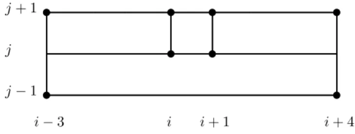
and, fori∈Zand j∈N, define (see Fig. 1)
Br(i, j) = [i∆r,(i+ 1)∆r)×[j∆r,(j+ 1)∆r),
(2.3)
e
Br(i, j) = Vr(i)×[(j−1)∆r,(j+ 1)∆r),
(2.4)
Vr(i, j) = Vr(i)× {(j−1)∆r},
(2.5)
with
(2.6) Vr(i) = [(i−3)∆r,(i+ 4)∆r).
TheBr(i, j)’s are calledr-blocks;Vr(i, j)plays the role of the pedestal ofBr(i, j). 3. Forr∈N0 andx∈Z, define the space interval
(2.7) Qr(x) = [x, x+C0r),
and, fort≥0, let
Ur(x, t) =
X
y∈Qr(x)
N(y, t), (2.8)
Eµ{Ur(x, t)} = µ|Qr(x)|=µC0r.
(2.9)
We say thatBr(i, j)isbad ifUr(x, t)< γrµC0rfor some(x, t)for whichQr(x)× {t}
i−3 i i+ 1 i+ 4
j−1
j j+ 1
t t
t t
t t
t t
Figure 1. Picture ofBr(i, j)(small square),Ber(i, j)(large rectangle)
andVr(i, j)(base of large rectangle), in units of∆r.
in a space interval of sizeCr
0 = ∆ 1/6
r ≪∆r somewhere inside the space-time block
e
Br(i, j). We say thatBr(i, j)isgood if it is not bad. 4. Forr, ℓ∈N0, define
φr(πb) = number of badr-blocks that intersect the space-time pathbπ,
(2.10)
Φr(ℓ) = sup
b π∈Ξ(ℓ,t)
φr(πb).
(2.11)
The principal result from [10] needed in Section 3 is the following.
Proposition 2.1. ([10, Proposition 8, p. 2441])For all K, ε0 >0 there exists an
r0=r0(K, ε0)such that for allr≥r0 there exists aµ0=µ0(K, ε0, r)such that for
allr≥r0 andµ≥µ0(K, ε0, r)there exists at0=t0(K, ε0, r, µ)such that
(2.12) PµΦr(ℓ)≥ε0C0−6r(t+ℓ) ≤2t
−K, r≥r
0, µ≥µ0, t≥t0, l∈N0.
In Appendix A we check the uniformity inµof the various estimates that went into the proof of Proposition 2.1.
3. Two propositions
The proof of Theorem 1.1 in Section 4 will be built on two propositions, which are stated and proved in Sections 3.1 and 3.4, respectively. The first proposition controls the number of bad r-blocks Br(i, j) that intersect the path of the green
particle up to time t, and its proof makes use of Proposition 2.1. The second proposition controls the number of goodr-blocksBr(i, j)that intersect the path of
the green particle up to timetand contain some point(x, t)that has no red particle coming from Vr(i, j). The proof of the second proposition requires two auxiliary
lemmas, which are stated and proved in Sections 3.2 and 3.3, respectively.
3.1. First proposition. Fort≥0, letE1(t)denote the event that the number of jumps by the green particle up to time t exceeds2t. Then there existC1, C2 >0
such that
(3.1) P{E1(t)} ≤C1e−C2t.
Indeed, the green particle has constant jump rate 1. Therefore the number of jumps up to timetis a Poisson random variable with meant, and the inequality is a standard large deviation bound for the Poisson distribution.
FixK, ε0>0andr0=r0(K, ε0)as in Proposition 2.1. Fort≥0, let
and
(3.3) Γr(t) =(i, j) : Br(i, j)∩ H(t)6=∅ .
The union of the r-blocks Br(i, j) with (i, j) ∈ Γr(t) is a fattened-up version of
the path of the green particle. We want to prove that, at large times t and high densities µ, the green particle sees many red particles close by. In fact, we will prove a somewhat stronger statement, namely, that with a large probability in an r-block Br(i, j) that is visited by the green particle all the space-time points are
visited by a red particle coming fromVr(i, j).
Fort≥0 andr∈N0, let
(3.4) eΓr(t) =
(i, j) : Br(i, j)∩ H(t)6=∅,Br(i, j)is bad , Proposition 3.1. ForK, ε0>0,r≥r0, µ≥µ0 andtsufficiently large,
(3.5) Pµ|Γe
r(t)| ≥3ε0C0−6rt =P
φr(H(t))≥3ε0C0−6rt ≤3t−K.
Proof. The equality follows from (2.10). To obtain the inequality, we apply Propo-sition 2.1. This tells us that forr≥r0,µ≥µ0,t≥t0andℓ∈N0, outside an event E2(t)of probability at most2t−K, we have
(3.6) Φr(ℓ) = sup
b π∈Ξ(ℓ,t)
φr(πb)≤ε0C0−6r(t+ℓ).
Furthermore, since each jump has size 1, if H(t)makes exactlyℓ jumps with 0≤
ℓ ≤ C(tlogt), then H(t) ∈ Ξ(ℓ, t). Hence, for logt ≥ 2 and outside the event
E1(t)∪ E2(t), we have
(3.7) φr(H(t))≤Φr(ℓ)≤ε0C0−6r(t+ℓ)≤3ε0C0−6rt.
Combine (3.1) and (3.7), and choosetso large thatC1e−C2t≤t−K, to get (3.5).
3.2. First auxiliary lemma. The time coordinate of the green particle is just time itself. Hence, ifT is some space-time set with projectionTeonto the time-axis, then the total time spent by the green particle inside T is at most the Lebesgue measure ofTe. In particular, ifH(t)intersects no more than3ε0C0−6rtbadr-blocks,
then the total time that is spent by the green particle in badr-blocks up to timet is at most
3ε0C0−6rt×C06r= 3ε0t.
(3.8)
We want to control the set of space-time points(x, t)in a goodr-blockBr(i, j)that
intersectsH(t)such that there is no red particle at(x, t)coming fromVr(i, j). We
want to show that also this set is small with a large probability. Let
(3.9) F(t) =σ{N(s) : 0≤s≤t},
be the sigma-field generated by the paths of all the red particles up to timet, and define
(3.10) Er(i, j) =
∃(x, t)∈ Br(i, j) :
Lemma 3.2. For allε1>0 andr∈N0 there exists aµ1=µ1(ε1, r)such that for
allµ≥µ1,i∈Z andj∈N, and uniformly on the event
(3.11) Nr(i, j) =
X
x∈Vr(i)
N(x,(j−1)∆r)≥γ0µ∆r
,
the following holds:
(3.12) PµEr(i, j)| F((j−1)∆r)} ≤ε1.
Proof. Note thatEr(i, j)depends only on the paths during the time interval[(j−
1)∆r,(j+ 1)∆r] of the red particles located in the space interval Vr(i) = [(i−
3)∆r,(i+ 4)∆r]at time(j−1)∆r. Since the red particles are interchangeable, the
conditional probability in (3.12) in fact only depends onN(x,(j−1)∆r),x∈Vr(i).
It is easy to see that if there are at least8∆rparticles inVr(i)at time(j−1)∆r,
then the conditional probabilityf(r)that these particles after time(j−1)∆rmove
in such a way that there is at least one of them at each point (x, t) ∈ Br(i, k)
satisfiesf(r)>0 (see Fig. 1). In particular,f(r)can be taken to be independent of the location of the red particles at time(j−1)∆r. In other words, on the event
(3.13) X
x∈Vr(i)
N(x,(j−1)∆r)≥8∆r,
we have
(3.14) Pµ[Er(i, j)]c | F((j−1)∆r)} ≥f(r).
Assume now that (3.11) holds. Then there are at least γ0µ∆r red particles in Vr(i) at time (j−1)∆r. Order these particles in an arbitrary way and partition
them intoq=⌊γ0µ/8⌋subsets of at least8∆r particles each, ignoring what is left
over. For each of these subsets the bound in (3.14) is valid. The event in the left-hand side of (3.12) occurs if and only if the event in the left-left-hand side of (3.14) fails for each of theq subsets. Since the paths of disjoint sets of red particles are independent, the left-hand side of (3.12) is therefore at most[1−f(r)]q. Now take µso large that[1−f(r)](γ0µ/8)−1≤ε
1, i.e.,
(3.15) µ≥µ1=
8
γ0
1 + logε1
log[1−f(r)]
.
Then (3.12) follows.
Note that because r 7→ γr is non-decreasing (see Appendix A) the result in
Lemma 3.2 also holds whenγ0 is replaced byγrin (3.11). In what follows we will
use the version withγ0.
3.3. Second auxiliary lemma. Abbreviate
(3.16) M =γ0µ∆r
and, fors∈N,i1, . . . , is∈Zandj1, . . . , js∈N, introduce the events
(3.17) Dr(i1, j1, . . . , is, js) = s
\
u=1
Nr(iu, ju).
Lemma 3.3. For allε1>0 andr∈N0 there exists aµ1=µ1(ε1, r)such that for
allµ≥µ1 the following are true.
(a) Let i1, . . . , is be such that their mutual differences are all ≥8. Then, for all j∈N,
PµnDr(i1, j, . . . , is, j)∩
∩su=1Er(iu, j)
o
≤Pµ{Dr(i1, j, . . . , is, j)}ε1s≤εs1, µ≥µ1(ε1, r).
(3.18)
(b) Let (i1, j1), . . . ,(is, js) be distinct such that the sum of their componentwise mutual differences are all≥10andj1, . . . , jsall have the same parity. Then
(3.19) PµnDr(i1, j1, . . . , is, js)∩∩su=1Er(iu, ju)o≤εs1, µ≥µ1(ε1, r).
Proof. (a) Write the left-hand side of (3.18) as a conditional expectation given
F((j−1)∆r). Since theju’s coincide, D(i1, j, . . . , is, j)only depends on the sites
inZ×[0,(j−1)∆r]. On the other hand,Er(i, j)only depends on the red particles
at the points in Z×[(j−1)∆r,(j+ 1)∆r). As in the first part of the proof of
Lemma 3.2, the conditional distribution of∩s
u=1Er(iu, j)given F((j−1)∆r)only
depends onN(x,(j−1)∆r),x∈Z. In fact, the conditional distribution ofEr(iu, j)
given F((j−1)∆r) only depends onN(x,(j−1)∆r),x∈Vr(iu). The collections
of red particles counted byN(x,(k−1)∆r),x∈Vr(iu), for differentiuare disjoint,
because the intervals Vr(iu) for different iu are disjoint. It follows thatEr(iu, j),
1 ≤u≤s, are conditionally independent givenF((j−1)∆r). Therefore the
left-hand side of (3.18) is bounded from above by
(3.20)
EµnPµDr(i1, j, . . . , is, j)| F((j−1)∆r)
×
s
Y
u=1
PµEr(iu, j)| F((j−1)∆r)
o .
However, on the eventD(i1, j, . . . , is, j), (3.11) holds fori∈ {i1, . . . , is}, and so we
see from Lemma 3.2 that
(3.21) Pµ{Er(iu, j)| F((j−1)∆r)} ≤ε1,
provided we takeµ≥µ1=µ1(ε1, r). This gives the first inequality in (3.18). The
second inequality is trivial.
(b) Put
(3.22) j= max{j1, . . . , js},
and suppose, without loss of generality, that there exists a 1≤u¯≤ssuch that (3.23) ju< j foru≤u¯ andju=j forj >u.¯
Note that
Dr(i1, j1, . . . , is, js)
=Dr(i1, j1, . . . , iu¯, ju¯)∩ Dr(iu¯+1, ju¯+1, . . . , is, js).
(3.24)
Note further that j1, . . . , ju¯ ≤ k−2, because all ju have the same parity. This
the proof of part (a), on the eventDr(i1, j1, . . . , iu¯, ju¯)we have
Pµ∩su=¯u+1Er(iu, ju)| F((j−1)∆r)
=Pµ∩s
u=¯u+1Er(iu, j)| F((j−1)∆r)
=
s
Y
u=¯u+1
PµEr(iu, j)| F((j−1)∆r) ≤εs1−u¯.
(3.25)
By taking the conditional expectation with respect toF((j−1)∆r)and using part
(a), we obtain
PµDr(i1, j1, . . . , is, js)∩∩su=1Er(iu, ju)
≤EµnDr(i1, j1, . . . , iu, ju)∩
∩¯uu=1Er(iu, ju) F((j−1)∆r)
o εs1−¯u
=PµnDr(i1, j1, . . . , iu¯, ju¯)∩∩uu¯=1Er(iu, ju)oεs1−u¯.
(3.26)
The proof can now be completed via a recursive argument. Indeed, the left-hand side of (3.26) deals with the probability of events indexed by spairs(iu, ju)with ju ≤ j and estimates this probability in terms of probabilities of events indexed
by pairs(iu, ju)with ju≤j−1 (and powers ofε1). We can therefore iterate the
estimate until it only contains powers ofε1.
3.4. Second proposition. Associated with H(t) is the collection of pairs Γr(t)
introduced in (3.3). Because the jumps of the green particle have size 1,Γr(t)when
viewed as a subset ofZ2 is connected, i.e., for any two pairs(i′, j′),(i′′, j′′)∈Γr(t)
there is a path in Γr(t)that runs from (i′, j′)to (i′′, j′′). In other words,Γr(t)is
a so-calledlattice animal containing the origin. We claim that with probability at least1−C1e−C2tthis lattice animal contains at mostℓ+t≤3tsites. Indeed, this
is so becauseHcan go from an r-block to an adjacentr-block in only two ways: (i) It crosses one of the time linesj∆r,j ∈N, without making a jump. Since
the time between two successive such crossings is ∆r, at most t/∆r such
crossings can occur up to timet.
(ii) It makes a jump. By the definition ofΞ(l, t), for Γ(t)∈ Ξ(ℓ, t) there are exactlyℓ such jumps up to timet.
Now, it is well known that there exist constants C3, C4 such that the number of
lattice animals of size 3t containing the origin is bounded from above by C3eC4t.
Thus, if we define
(3.27) Wr(t) = collection of possible setsΓr(t),
then we have proved that, with probability at least1−C1e−C2t,
(3.28) |Wr(t)| ≤C3eC4t.
Ther-block corresponding to a point(i, j)∈Γr(t)can be either bad or good. We
will call a pair (i, j) ∈Γr(t) bad or good according asBr(i, j) is bad or good. It
is immediate from (2.10–2.12) that, outside the eventE1(t)∪ E2(t), the number of bad r-blocks in Γr(t) is at most 3ε0C0−6rt. Together with (3.8), this proves that H(t)spends only a small fraction of its time in bad blocks. We therefore only need to deal with the subset of good pairs in Γr(t). Of particular interest will be the
following subset ofΓr(t):
whereE∗
r(i, j)is the event that Br(i, j)contains a point that is not visited by any
of the red particles coming fromVr(i, j).
Proposition 3.4. There exist a C1, . . . , C6 > 0 such that for all 0 < ε1 < 1,
µ≥µ1(ε1, r)andt sufficiently large,
(3.30) Pµ{|Λr(t)| ≥ε1t} ≤C1e−C2t+C3eC4t23tε1⌊C5+C6ε1t⌋.
Proof. The idea of the proof is to partition the event{|Λr(t)| ≥ε1t}into a union of
subevents of the form analyzed in Lemma 3.3, to estimate the probability of each of these subevents by means of Lemma 3.3, and afterwards sum over all the ways to do the partition.
Consider a sample point for which |Λr(t)| ≥ ε1t, but for which E1(t) does not
occur (i.e., the green particle makes≤2tjumps up to timet). Then, sinceΛr(t)⊂
Γr(t)⊂Z2, there exist at most⌊C5+C6ε1t⌋points(iu, ju)∈Λr(t)with the sum
of their componentwise differences all≥10, withC5, C6>0 independent ofΛr(t)
andµ. SinceBr(i, j)is good when(i, j)∈Λr(t), we have
(3.31) X
x∈Vr(i)
N(x,(j−1)∆r)≥γrµ∆r≥γ0µ∆r=M,
i.e., the eventNr(i, j)defined in (3.11) occurs. Let
(3.32) Λbr(t) =(i, j) : Br(i, j)∩ H(t)6=∅,Nr(i, j)andEr∗(i, j)occur .
ThenΛbr(t)⊃Λr(t), and so the points(iu, ju),1≤u≤C5+C6ε1t, all lie inΛbr(t).
This means that Dr(i1, j1, . . . , is, js) occurs with s =⌊C5+C6ε1t⌋and M as in
(3.16) (recall (3.17)). In addition,
(3.33) ∩su=1Er(iu, ju)
occurs (recall (3.12)).
The above observations show that|Λr(t)|> ε1tcan occur for µ≥µ1(ε1, r)and
tlarge enough only if, for some possible choice of the (iu, ju)’s,
(3.34) D(i1, j1, . . . , is, js)∩
∩su=1Er(iu, ju)
occurs. Lemma 3.3 shows that, for any permissible choice of the (iu, ju)’s, the
probability of (3.34) is at mostεs
1. Consequently,
Pµ{|Λr(t)| ≥ε1t}
≤X
Γr
X
Θ⊂Γr
PµDr(i1, j1, . . . , is, js)∩∩su=1Er(iu, ju)
≤X
Γr
X
Θ⊂Γr
εs1,
(3.35)
providedµ≥µ1(ε1, r)andt is sufficiently large. Here, the sum overΓr runs over
all possible realizations of the random set Γr(t), andΘruns over all choices of the
(iu, ju)’s whose sum of componentswise differences are all≥10, and are such that
theju’s all have the same parity.
Now assume that our sample point lies outside E1(t), which happens with a probability at least1−C1e−C2t. Then
(3.36) X
Θ⊂Γr
1≤23t,
because|Γr| ≤3t, as we saw before. Moreover, by (3.28), we have
(3.37) X
Γr
1≤C3eC4t,
sinceΓr is a lattice animal that contains the origin and has size at most3t.
Com-bining these estimates, we find that forµ≥µ1(ε1, r)andtsufficiently large,
(3.38) Pµ{|Λr(t)| ≥ε1t} ≤C1e−C2t+C3eC4t23tε1⌊C5+C6ε1t⌋.
4. Proof of Theorem 1.1
Proof. With Propositions 3.1 and 3.4 in hand, the proof of Theorem 1.1 is routine. We distinguish four possible types ofr-blocks,
(4.1) (bad,occupied), (bad,vacant), (good,occupied), (good,vacant), where an r-blockBr(i, j)is calledoccupied whenEr∗(i, j)c occurs, i.e., every point
in Br(i, j) is visited by a red particle coming from Vr(i, j), and is called vacant
otherwise. The number ofr-blocks of type (bad,occupied) that intersectH(t)will be denoted byNr(t; (bad,occupied)), and similarly for the other types.
We have shown in Proposition 3.1 that
Nr(t; (bad)) =Nr(t; (bad,occupied)) +Nr(t; (bad,vacant))
≤ |eΓr(t)| ≤3ε0C0−6t
(4.2)
outside an event of probability at most3t−K, providedK, ε
0>0, µ≥µ0(K, ε0, r)
andt is sufficiently large. We have further shown in Proposition 3.4 that
(4.3) Nr(t; (good,vacant)) =|Λr(t)| ≤ε1t
outside an event of probability at mostC1e−C2t+C3eC4t23tε⌊1C5+C6ε1t⌋, provided
0 < ε1 < 1, µ ≥ µ1(ε1, r) and t is sufficiently large. Since we can choose ε0, ε1
arbitrarily small, it follows from (4.2–4.3) that there exists a function µ 7→ bt(t)
from(0,∞)to itself such that
1
t
N(r, t; (bad,vacant)) +N(r, t; (good,vacant))→0
inPµ-probability asµ, t→ ∞such thatt≥bt(µ). (4.4)
According to the projection argument given in the lines just before (3.8), this in turn implies that
1
t
total time thatH(t)is in an r-block
that is (bad,occupied) or (good,occupied)→1
inPµ-probability asµ, t→ ∞such thatt≥bt(µ). (4.5)
Finally, let L be the infinitesimal generator of the random walk performed by the green particle when the space-time trajectories of the red particles, given byN defined in (1.1), are fixed. Then
(4.6) (LI)(x, t) =
(
v′ ifN(x, t)≥1,
v′′ ifN(x, t) = 0, I(x, t) = (x, t).
Recall G defined in (1.3). By a standard martingale property, we have (see e.g. [10](Lemma 10))
(4.7) lim
t→∞
1
t
G(t)−
Z t
0
(LI)(G(s), s)ds
= 0, Pµ-a.s.
Combining (4.5) and (4.6), we see that (LI)(G(s), s) = v′ on a set ofs-values in
[0, t]that converges inPµ-probability to all of[0, t]. Therefore Theorem 1.1 follows
from (4.7).
Appendix A. Uniformity in µ
Our main focus in this Appendix is on [10, Section 4], and we will adopt the notation used there. Consequently, the arguments given below cannot be read independently. Moreover, in [10] at some places a choice of parameters depends on µ. However, as we will check below, this dependence does not requireµ→ ∞.
Note that in Proposition 2.1 we choose the parameters in the orderK, ε0, r, µ, t.
Since in Theorem 1.1 we let t→ ∞ first, it suffices to check that inequalities hold for larget whenµis fixed.
1. As shown in [10, Sections 1 and 4], C0 and (γr)r∈N0 mentioned in Section 2,
Part 2, are chosen such that
0< γ0Q∞j=11−2−j/4
−1 ≤ 12, (A.1)
γ1=γ0, γr+1=γ0Qrj=1
1−C0−j/4−1, r∈N,
(A.2)
whereC0 is taken so large that, for allr∈N,
C0−r/2−1−C4rlogC0
Cr
0
1−e−C−r/2
0 [1−C−r/4
0 ]−1≤ −21C
−3r/4
0 ,
(A.3)
9C012(r+1)exp[−12γ0µC
r/4 0 ]≤1,
(A.4)
whereC4 is the constant in [10, Lemma 5] (andµtakes over the role ofµAin [10]).
It is not hard to check in the proof of [10, Lemma 5] thatC4in (A.3) can be chosen
independently ofµ. As was already checked in [10], C4 is also independent of C0,
so that we can choose(γr)r∈N0 andC0independently ofC4as well. In other words,
once a value for C4 has been determined on the basis of [10, Lemma 5], we may
safely letµ→ ∞.
2. The next place were the uniformity inµneeds to be checked is [10, Eq. (4.16– 4.17)]. For any choice of K > 0 and K4 >0, we define R(t)by [10, Eq. (4.16)],
the position at timet of the right-most red particle. The first three inequalities in [10, Eq. (4.17)] continue to be valid, uniformly in µ. We can chooseK4 to make
also the fourth inequality in [10, Eq. (4.17)]valid, uniformly inµ, by observing that Ur(x, t)in (2.8) has a Poisson distribution with meanµC0r, so that, for anyθ >0,
Pµ{U
r(x, t)≤ 12µC0r}=Pµ
e−θUr(x,t)≥e−12θµCr0
≤e12θµC
r
0Eµ n
e−θUr(x,t)
o
=e12θµC
r
0e−µCr0(1−e−θ). (A.5)
Pickθ >0so small that(1−e−θ)−1 2θ≥
1
4θ, to obtain
X
r≥R(t)
PUr(x, t)≤ 12µC0r ≤e− 1 4θµC
R(t)
0 X
r≥R(t)
e−14θµC
r−R(t) 0
≤K20e− 1 4θµC
R(t) 0 (A.6)
for some constantK20that depends onC0only, as long asµis bounded away from
0, say µ ≥ 2. It is immediate from this estimate that the sum of P{Ur(x, t) ≤
1
2µC0r}over(x, s), withs∈[−∆r, t+ ∆r)integer andxsuch thatQr(x)intersects
C(tlogt+ 3∆r), when summed overr≥R(t)is no more thant−K, providedµ≥2
and K4 (or, equivalently, R(t)) is sufficiently large, independently of µ. Thus, we
conclude that [10, Eq. (4.17)] is valid uniformly inµ≥2.
3. [10, Lemmas 5–6] remain valid for µ > 0, while also [10, Lemma 7] remains valid, even with C5 independent of µ, as long as µ is bounded away from 0, say
µ≥2. Indeed, the inequality in [10, Eq. (4.29)] is based on the estimate
(A.7) E{T}=λν2ρ
r+1≤22λ≤62
t+ℓ ν∆r+1
and on Bernstein’s inequality (see [10, Eq. (4.37) and subsequent lines] for the appropriate notation. In the case of a binomial random variable T corresponding toλν2 trials with success probabilityρ, Bernstein’s inequality gives
(A.8) P{T ≥αE{T}}=P{T−E{T} ≥(α−1)E{T}} ≤exp−1
4(α−1)E{T}
forα >1 (see [6, Exercise 4.3.14]. Thus, [10, Lemma 7] holds uniformly inµ≥2. 4. It remains to verify the uniformity of [10, Proposition 8], i.e., Proposition 2.1 above. To do so, we consider a sample point where [10, Eq. (4.39)] holds for all µ≥2,r≥R(t)and ℓ∈N0, and where [10, Eq. (4.40)] holds independently ofµ.
Then there exists anr0 independent ofµ≥2 such that [10, Eq. (4.41)] holds all
r∈[r0, R(t)−1],ℓ∈N0, µ≥2 andtsufficiently large. Moreover, these estimates
hold for all sample points outside an event of probability at most
(A.9) t−K+ R(Xt)−1
r=1
X
ℓ∈N0
exph−(t+ℓ)C5κ0exp
h
1 2γrµC
1 4 0
ii
≤2t−K.
This proves Proposition 2.1 with the required uniformity inµ. The only requirement forr0is that the last inequality in [10, Eq. (4.41)] holds. Thus, we only need
(A.10) 6κ0[C0]12+6rexp
h
−γ0µ
4 C
1 4r 0
i
≤ε0.
Acknowledgements. Part of the research for this paper was carried out in the Spring of 2009, during visits by the authors to the Mittag-Leffler Institute in Djur-sholm in Sweden and to the Mathematical Institute of Leiden University in The Netherlands. The authors thank the Swedish Research Council for support. FdH is supported by ERC Advanced Grant 67356 VARIS. VS is supported by CNPq (Brazil) grants 308787/11-0 and 484801/11-0 and by Edital Faperj grant CNE 2011. VS also thanks the ESF Research Network Program RGLIS for support.
References
[1] L. Avena, T. Franco, M. Jara and F. Völlering, Symmetric exclusion as a random environ-ment: hydrodynamic limits. [arXiv:1211.3667]
[2] L. Avena, F. den Hollander and F. Redig, Law of large numbers for a class of random walks in dynamic random environments, Electr. J. Probab. 16 (2011) 587–617.
[3] L. Avena, F. den Hollander and F. Redig, Large deviation principle for one-dimensional random walk in dynamic random environment: attractive spin-flips and simple symmetric exclusion, Markov Proc. Relat. Fields 16 (2010) 139–168.
[4] L. Avena, R. dos Santos and F. Völlering, Transient random walk in symmetric exclusion: limit theorems and an Einstein relation, to appear in ALEA. [arXiv:1102.1075]
[5] A. Bandyopadhyay and O. Zeitouni, Random walk in dynamic Markovian random environ-ment, ALEA 1 (2006) 205–224.
[6] Y.S. Chow and H. Teicher, Independence, Interchangeability, Martingale Series(3rd. ed.), Springer Texts in Statistics, Springer, New York, 1997.
[7] D. Dolgopyat, G. Keller and C. Liverani, Random walk in Markovian environment, Ann. Prob. 36 (2008) 1676-1710.
[8] F. den Hollander and R. dos Santos, Scaling of a random walk on a supercritical contact process, to appear in Ann. I. Henri Poincaré. [arXiv:1209.1511]
[9] F. den Hollander, R. dos Santos and V. Sidoravicius, Law of large numbers for non-elliptic random walks in dynamic random environments, Stoch. Proc. Appl. 123 (2012) 156–190. [10] H. Kesten and V. Sidoravicius, The spread of a rumor or infection in a moving population,
Ann. Prob. 33 (2005) 2402–2462.
[11] F. Redig and F. Völlering, Random walks in dynamic random environments: a transference principle, to appear in Ann. Prob. [arXiv:1211.0830].
[12] F. Solomon, Random walks in a random environment, Ann. Prob. 3 (1975) 1–31.
Mathematical Institute, Leiden University, P.O. Box 9512, 2300 RA Leiden, The Netherlands
E-mail address: [email protected]
Malott Hall, Cornell University, Ithaca, NY.,14853, USA E-mail address: [email protected]
IMPA, Estrada Dona Castorina 110, Jardim Botanico, Cep 22460-320, Rio de Janeiro, RJ, Brasil
E-mail address: [email protected]