Spherical Cap Packing Asymptotics
and Rank-Extreme Detection
Kai Zhang
Abstract—We study the spherical cap packing problem with a probabilistic approach. Such probabilistic considerations result in an asymptotic sharp universal uniform bound on the maximal inner product between any set of unit vectors and a stochastically independent uniformly distributed unit vector. When the set of unit vectors are themselves independently uniformly distributed, we further develop the extreme value distribution limit of the maximal inner product, which characterizes its uncertainty around the bound.
As applications of the above asymptotic results, we derive (1) an asymptotic sharp universal uniform bound on the maximal spurious correlation, as well as its uniform convergence in distribution when the explanatory variables are independently Gaussian distributed; and (2) an asymptotic sharp universal bound on the maximum norm of a low-rank elliptically dis-tributed vector, as well as related limiting distributions. With these results, we develop a fast detection method for a low-rank structure in high-dimensional Gaussian data without using the spectrum information.
Index Terms—Spherical cap packing, extreme value distribu-tion, spurious correladistribu-tion, low-rank detection and estimadistribu-tion, high-dimensional inference.
I. INTRODUCTION
In modern data analysis, datasets often contain a large number of variables with complicated dependence structures. This situation is especially common in important problems such as the relationship between genetics and cancer, the association between brain connectivity and cognitive states, the effect of social media on consumers’ confidence, etc. Hundreds of research papers on analyzing such dependence have been published in top journals and conferences proceedings. For a comprehensive review of these challenges and past studies, see [1].
One of the most important measures on the dependence be-tween variables is the correlation coefficient, which describes their linear dependence. In the new paradigm described above, understanding the correlation and the behavior of correlated variables is a crucial problem and prompts data scientists to develop new theories and methods. Among the important challenges of a large number of variables on the correlation, we focus particularly on the following two questions:
• The maximal spurious sample correlation in high dimensions.The Pearson’s sample correlation coefficient between two random variables X and Y based on n
Kai Zhang is with the Department of Statistics and Operations Research, University of North Carolina, Chapel Hill (e-mail: [email protected])
observations can be written as
b
C(X, Y) =
Pn
i=1(Xi−X¯)(Yi−Y¯) q
Pn
i=1(Xi−X¯)2
q Pn
i=1(Yi−Y¯)2 (I.1) whereXi’s andYi’s are thenindependent and identically distributed (i.i.d.) observations ofX andY respectively, and X¯ and Y¯ are the sample means of X and Y
respectively. The sample correlation coefficient possesses important statistical properties and was carefully studied in the classical case when the number of variables is small compared to the number of observations. How-ever, the situation has dramatically changed in the new high-dimensional paradigm [1, 2] as the large number of variables in the data leads to the failure of many conventional statistical methods. For sample correlations, one of the most important challenges is that when the number of explanatory variables, p, in the data is high, simply by chance, some explanatory variable will appear to be highly correlated with the response variable even if they are all scientifically irrelevant [3, 4]. Failure to recognize such spurious correlations can lead to false scientific discoveries and serious consequences. Thus, it is important to understand the magnitude and distribution of the maximal spurious correlation to help distinguish signals from noise in a large-psituation.
• Detection of low-rank correlation structure.Detecting a low-rank structure in a high-dimensional dataset is of great interest in many scientific areas such as signal pro-cessing, chemometrics, and econometrics. Current rank estimation methods are mostly developed under the factor model and are based on the principal component analysis (PCA) [5–21], where we look for the “cut-off” among singular values of the covariance matrix when they drop to nearly 0. These methods also usually assume a large sample size. However, in practice often a large number of variables are observed while the sample size is limited. In particular, PCA based methods will fail when the number of observations is less than the rank. Moreover, although we may get low-rank solutions to many problems, more detailed inference on the rank as a parameter is not very clear. Probabilistic statements on the rank, such as confidence intervals and tests, would provide useful information about the accuracy of these solutions. The computation complexity of the matrix calculations can be an additional issue in practice. In summary, it is desirable to have a fast detection and inference method of a low-rank structure in high dimensions from a small sample.
Our study of the above two problems starts with the following question: Supposeppoints are placed on the unit sphereSn−1
in Rn. If we now generate a new point on Sn−1 according
to the uniform distribution over the sphere, how far will it be away from these existingppoints?
Intuitively, this minimal distance between the new point and the existing ppoints should depend onn andp, in a manner that it is decreasing in pand increasing in n. Yet, no matter how these existingppoints are located, this new point cannot get arbitrarily close to the existingppoints due to randomness. In other words, for any n and p, there is an intrinsic lower bound on this distance that the new point can get closer to the existing points only with very small probability.
Studies of this intrinsic lower bound in the above question have a long history under the notion of spherical cap packing, and this question has been one of the most fundamental questions in mathematics [22–24]. In fact, this question is closely related to the 18th question on the famous list from David Hilbert [25]. This question is also a very important problem in information theory and has been studied in coding, beamforming, quantization, and many other areas [26–33].
Besides the importance in mathematics and information the-ory, this question is closely connected to the two problems that we propose to investigate. For instance, the sample correlation betweenX andY can be written as the inner product
b
C(X, Y) =h X−X¯1n kX−X¯1nk2
, Y −
¯
Y1n
kY −Y¯1nk2
i, (I.2)
whereX = (X1, . . . , Xn), Y = (Y1, . . . , Yn), and1n is the vector in Rn with all ones. In general, if we observen i.i.d. samples from the joint distribution of (X1, . . . , Xp, Y), the sample correlations between Xj’s and Y can be regarded as inner products inRnbetween thepunit vectors corresponding to Xj’s and another unit vector corresponding to Y. Note that these unit vectors are all orthogonal to the vector 1n due to the centering process. Thus, they lie on an “equator” of the unit sphere Sn−1 in
Rn, which is in turn equivalent to Sn−2. Through this connection, the problem about the
maximal spurious correlation is equivalent to the packing of the inner products, and existing methods and results from the packing literature can be borrowed to analyze this problem. In this paper, we particularly focus on probabilistic statements about such packing problems.
An important advantage of this packing perspective is a view of data that is free of an increasing p. Suppose we view the data as n points in a p-dimensional space, then if pexceeds
n, all the n points will lie on a low-dimensional hyperplane inRp. This degeneracy forces us to change the methodology towards statistical problems, i.e., changing from the classical statistical methods to recent high-dimensional methods [34, 35]. However, if we view the data aspvectors inRn, then we will never have such a degeneracy problem. No matter how largepis, a packing problem is always a well-defined packing problem. Neither the theory nor the methodology needs to be changed due to an increase in p. Thus, with the packing perspective, theory and methodology can be set free from the restriction of an increasing p.
We summarize below our results on the asymptotic theories of the maximal inner products and spurious correlations. One major advantage of the packing approach is that instead of usual iterative asymptotic results which set p=p(n)and let
n→ ∞,our convergence results are uniform inn, which leads to double limits in both nandp.
• We characterize the largest magnitude of independent inner products (or spurious correlations) through an asymptotic bound. This bound is universal in the sense that it holds for arbitrary distributions of Lj’s (or that of Xj’s). This bound is uniform in the sense that it holds asymptotically in p but is uniform over n. This bound is sharp in the sense that it can be attained, especially when the unit vectors Lj’s are i.i.d. uniform (or whenXj’s are independently Gaussian). Thus, in an analogy, this bound is to the distribution of independent inner products (or to that of spurious correlations) as the fundamental bound √2 logpis to the p-dimensional Gaussian distribution [36]. We refer this bound as the Sharp Asymptotic Bound for indEpendent inner pRoducts (or spuRious corrElations), abbreviated as the SABER (or SABRE).
• In the special important case when the set of unit vectors are i.i.d. uniformly distributed (or when Xj’s are inde-pendently Gaussian distributed), we show the sharpness of the SABER (or SABRE) and describe a smooth phase transition phenomenon of them according to the limit of
logp
n . Furthermore, we develop the limiting distribution by combing the packing approach with extreme value the-ory in statistics [36, 37]. The extreme value thethe-ory results accurately characterize the deviation from the observed maximal magnitude of independent inner products (or that of spurious correlations) to the SABER (or SABRE). One important feature of these results is that they are not only finite sample results but also are uniform-n
-large-p asymptotics that are widely applicable in the high-dimensional paradigm.
association.
Based on the asymptotic results on the degenerate elliptical distributions, we show that one can make statistical inference on a low-rank through the distributions of the extreme value as a statistic. One feature of this procedure is that it does not require the spectrum information from PCA. Thus, the new method works when n < d, when PCA based methods fail to work. It is also computationally fast since no matrix multi-plication is needed in the algorithm. These advantages allow a fast detection of a low-dimensional correlation structure in high-dimensional data.
A. Related Work
We are not able to find similar probabilistic statements on uniform-n-large-p asymptotics. The following statistical papers are related to the study on the maximal spurious correlation.
• In [4], the authors obtain a result on the order of the maximal spurious correlations in the regime that lognp →
0.Through the packing approach, we derive the explicit limiting distribution of the extreme spurious correlations for entire scope ofn andp.
• In [39], the authors develop a threshold for marginal correlation screening with large p and small n. The threshold appears in a similar form as the SABRE. We note two major differences between the results: (1) The results in [39] focus on the regime when lognp → ∞(i.e., when the threshold converges to 1), while our asymptotic results cover the entire scope ofnandp, and the SABRE is shown to be valid from 0 to 1; (2) we derive the explicit limiting distribution of the maximal spurious correlation in the most important case when the variables are i.i.d. Gaussian.
• In [40–42], the minimal pairwise angles between i.i.d. uniformly random points on spheres are considered. A similar phase transition is described, and results on the limiting distribution are developed. We note two major differences between their results and ours: (1) Due to different motivations of the research, we focus on the marginal correlation between one response variable and
p explanatory variables. We also develop a universal uniform bound for marginal correlations. (2) The extreme limiting distributions in their papers are stated separately according to if the limit of lognp is 0, a proper constant, or ∞.From the packing perspective, we are able to state the convergence in a uniform manner with standardizing constants that are adaptive in n and p. Since in real data, the limit of lognp is usually not known, this uniform convergence with adaptive standardizing constants makes the result easy to apply in practice.
• During the review process of this paper, we noticed the results in [43] which focus on the coupling and bootstrap approximations of the maximal spurious correlation when
log7p
n →0. Again our different focus is on explicit lim-iting distributions with adaptive standardizing constants from the packing perspective.
We are not able to find existing literature on the rank-extreme association. To evaluate the performance of our low-rank detection method, we compare our method with the algorithm in [14] which studies a similar problem. During the review process of the paper, we also noticed recent work by [21]. The most important difference from these papers is that they focus on the case whennandpare comparable and both large, while we consider the case whennis small and pis large.
B. Outline of the Paper
In Section II, we derive the asymptotic bound on the spherical packing problem, as well as that of the maximal spurious correlation and the related extreme value distribu-tions. In Section III, we describe the rank-extreme association of elliptically distributed vectors. In Section IV we develop a fast detection method of a low-rank by using the rank-extreme association reversely. In Section V, we study the performance of the detection method through simulations. We conclude and discuss future work in Section VI.
II. ASYMPTOTICTHEORY OF THESPHERICALCAP
PACKINGPROBLEM
A. The Sharp Asymptotic Bound for independent inner prod-ucts (SABER) and Spurious Correlations (SABRE)
We first observe that as described in [44], when
U is uniformly distributed over Sn−1, |hL,Ui|2 ∼ Beta 1
2,
n−1 2
,∀L ∈ Sn−1. By borrowing strength from the
packing literature [22, 26] on the total area of non-overlap spherical caps onSn−2, we develop the following theorem on
a sharp asymptotic bound for independent inner products. Theorem II.1. Sharp Asymptotic Bound for Independent Inner Products (SABER).
For arbitrary deterministic unit vectors L1, . . . ,Lp and a uniformly distributed unit vector U over Sn−1, the random variableMp,n= max1≤j≤p|hLj,Ui|satisfies that∀δ >0,
P
Mp,n> q
(1 +δ)(1−p−2/(n−1))
≤ √
2p1/(n−1)exp
−1
2δ(n−1)(p
2/(n−1)−
1)
p
π(1 +δ)(n−1)(p2/(n−1)−1) .
(II.1)
Therefore,∀δ >0, asp→ ∞,
sup n≥2
P
Mp,n> q
(1 +δ)(1−p−2/(n−1))
→0. (II.2)
In particular, ifn→ ∞,then we have the double limit lim
p,n→∞P
Mp,n≤ p
1−p−2/(n−1)
= 1. (II.3)
Theorem II.1 provides an explicit answer to the question at the beginning of Section I with a probabilistic statement: No matter how Lj’s are located on the unit sphere, the magnitude of the inner products (or cosines of the angle) between theseppoints and a uniformly random point cannot exceedp1−p−2/(n−1)with high probability for largep.This
The SABER possesses the following important properties: 1) This bound is universal in the sense that it holds for any
configuration of Lj’s.
2) This bound is uniform in the sense that it holds uniformity for n≥2.
3) This bound is sharp in the sense that it can be attained for some configuration of Lj’s, especially when Lj’s are i.i.d. uniformly distributed, as will be discussed in Section II-B.
Thus, in an analogy, the SABERp1−p−2/(n−1)is to the
dis-tributions of the independent inner products as the fundamental bound √2 logpis to thep-dimensional Gaussian distribution. A technical note here is that when n is finite, the fraction
2
n−1 in the exponent ofpcan be replaced by 2
n−n1 with any
fixed integer 0 < n1 < n. This change would not alter the
asymptotic result in p due to a uniform convergence in the proof. The numbern1only has an effect when the dimensionn
is finite. For example, see [39] for a similar but different bound when n is fixed. We focus on the bound p1−p−2/(n−1)
due to its connection to theBeta 12,n−21
distribution. When
n→ ∞,all these bounds are equivalent.
Another technical note is that although Theorem II.1 is for a deterministic set of Lj’s, we note here that this set of unit vectors can be random as well. As long as Lj’s are stochastically independent of U,Theorem II.1 can be applied to randomLj’s by a conditioning argument on any realization of Lj’s.
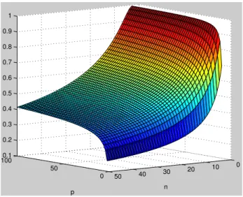
Figure 1 illustrates the SABER p1−p−2/(n−1) in
The-orem II.1 as a function of n and p. It can be seen that the SABER has a range of (0,1) as an increasing function in p
and a decreasing function in n.
0 50
100
0 10 20 30 40 50 0.1
0.2 0.3 0.4 0.5 0.6 0.7 0.8 0.9 1
n p
Fig. 1. The SABERp1−p−2/(n−1)for3≤n≤50and2≤p≤100. The SABER ranges from 0 to 1. The regions of the same color represent the smooth phase transition curves lognp ≈ β forβ > 0 as described in Section II-B.
Due to the connection between sample correlations and the inner products (I.2), this bound is immediately applicable to spurious correlations. Suppose Y = (Y1, . . . , Yn) records n i.i.d. samples of a Gaussian variable Y,then it is well-known (see [44]) that Y−Y¯1n
kY−Y¯1nk2 is a uniformly distributed unit vector
overSn−2. Thus, we have the following bound on the maximal
spurious correlation.
Corollary II.2. Sharp Asymptotic Bound for Spurious Correlations (SABRE).
Suppose we observe n i.i.d. samples of arbitrary random variables X1, . . . , Xp and a Gaussian variable Y that is independent ofXj’s. The maximal absolute sample correlation
MXY = max1≤j≤p|Cb(Xj, Y)| satisfies that ∀δ > 0, as
p→ ∞,
sup n≥3
P
MXY >
q
(1 +δ)(1−p−2/(n−2))
→0. (II.4)
In particular, ifn→ ∞, then we have the double limit
lim p,n→∞P
MXY ≤
p
1−p−2/(n−2)
= 1. (II.5) Similarly as the interpretation for the SABER, the impli-cation of the SABRE is as follows: Uniformly for n ≥ 3,
no matter how the p variables X1, . . . , Xp are distributed, the magnitude of the sample correlations betweenXj’s and a GaussianY cannot exceed the SABRE with high probability for largep.Note here that in practice, the requirement of Gaus-sianity of Y can be easily relaxed through a transformation of distributions. Since the SABRE is universal, uniform, and sharp as the SABER, this bound provides a way to distinguish true signals from spurious correlations. We shall investigate this application in future work.
B. Limiting Distributions in the i.i.d. Case
In this section, we describe the asymptotics of the maximal inner product when Lj’s are i.i.d. uniformly distributed and the asymptotics of spurious correlations when Xj’s are in-dependently Gaussian distributed. We first observe that when
Lj’s are i.i.d. uniformly unit vectors overSn−1,then for any random unit vectorU that is independent ofLj’s, we have the following two properties about the inner productshLj,Ui|U: 1) Conditioning onU,the variables hLj,Ui|U’s are
inde-pendent sinceLj’s are independent;
2) For each j, the variable |hLj,Ui|2|U is distributed as Beta 12,n−21. Since this conditional distribution does not depend on U, it implies that unconditionally
|hLj,Ui|2 is stochastically independent ofU.
From these two properties, we conclude that unconditionally,
|hLj,Ui|2’s are i.i.d.Beta 12,n−21
distributed. We thus show the sharpness of the SABER and SABRE by studying the maximum of i.i.d.Beta(1
2,
n−1
2 )variables.
Theorem II.3.
1) (Sharpness of SABER)
SupposeLj’s are i.i.d. uniformly distributed over the(n− 1)-sphereSn−1,then for arbitrary random unit vectorU that is independent ofLj’s, uniformly for all n≥2, as
p → ∞, the random variable Mp,n = maxj|hLj,Ui| has the following convergence:
Mp,n/
p
i.e.,∀δ >0, asp→ ∞,
sup n≥2
P(|Mp,n2 /(1−p−2/(n−1))−1|> δ)−→0. (II.7)
2) (Sharpness of SABRE)
Similarly, suppose we observeni.i.d. samples of indepen-dent Gaussian variables X1, . . . , Xp and an arbitrarily distributed random variable Y that is independent of Xj’s. Consider the maximal absolute sample correlation
MXY = max1≤j≤p|Cb(Xj, Y)|.Uniformly for alln≥3, as p→ ∞,we have
MXY/
p
1−p−2/(n−2)prob.−→ 1. (II.8)
Theorem II.3 shows the sharpness of the SABER and the SABRE. It further describes a smooth phase transition ofMp,n (also MXY) depending on the limit of lognp :
(i) If limp→∞logp/n = ∞, then Mp,n prob.
−→ 1 and
Mp,n/
p
1−p−2/(n−1)prob.−→ 1.
(ii) If limp→∞logp/n = β for fixed 0 < β < ∞, then
Mp,n prob.
−→ √1−e−2β.
(iii) If limp→∞logp/n = 0, then Mp,n prob.
−→ 0 and
Mp,n/
p
2 logp/nprob.−→1.
Note in particular that when limp→∞logp/n = 0, the SABRE satisfies
p
1−p−2/(n−2)
=p1−e−2 logp/(n−2) ∼p1−(1−2 logp/n) =p2 logp/n.
(II.9)
The rate p2 logp/n has appeared in hundreds of books and papers and is very-well known in high-dimensional statistics literature [35]. However, it is just a special case of the general rate p1−p−2/(n−2), which is obtained through the packing
perspective. This fact demonstrates the power of this packing approach. In Figure 1, the smooth phase transition curves
logp
n ≈β are represented as regions of the same color. Below are some geometric intuitions on why the phase transition depends on the limit of lognp: Note that the number of orthants in Rn is 2n and is growing exponentially in n. Therefore, if the growth ofpis faster than the exponential rate in n, then the punit vectors on Sn−1 would be so “dense”
that they would cover the sphere, making the magnitude of the maximal inner product converging to 1; if the growth of
pis exponential inn, then there would be a constant number (depending on the limit of lognp) of points in each orthant, so that the new random point would stay around some proper angle to the existing points; if the growth of p is slower than the exponential rate, then many orthants would be empty of points asymptotically, thus the new random point can be almost orthogonal to the existing points.
WhenLj’s are i.i.d. uniformly distributed or whenXj’s are independently Gaussian, by combining the results in packing literature [22, 26] and classical extreme value theory [36, 37], we further develop the following uniform convergence in distribution of the corresponding maxima.
Theorem II.4.
1) (Limiting Distribution of the Maximal Independent Inner Product)
SupposeLj’s are i.i.d. uniformly unit vectors overSn−1. For arbitrary random unit vectorU that is independent ofLj’s, considerMp,n= max1≤j≤p|hLj,Ui|. Let
ap,n= 1−p−2/(n−1)cp,n, bp,n= 2
n−1p
−2/(n−1)c
p,n,
where cp,n = n−21B 12,n2−1p1−p−2/(n−1)
2/(n−1)
is a correction factor withB(s, t)being the Beta function. Then for any fixedx, as p→ ∞,
sup n≥2
P
Mp,n2 −ap,n
bp,n
< x
−I
x > n−1
2
−exp
−
1− 2
n−1x
(n−1)/2
I
x≤n−1
2
→0.
(II.10)
In particular, ifn→ ∞andp→ ∞,then for any fixed x, we have the double limit
P
M2
p,n−ap,n
bp,n
< x
→exp −e−x
. (II.11)
2) (Limiting Distribution of the Maximal Spurious Cor-relation)
Similarly, suppose we observeni.i.d. samples of indepen-dent Gaussian variables X1, . . . , Xp and an arbitrarily distributed random variable Y that is independent of Xj’s. Consider the maximal absolute sample correlation
MXY = max1≤j≤p|Cb(Xj, Y)|.Then for any fixedx, as
p→ ∞,
sup n≥3
P
MXY2 −ap,n−1 bp,n−1
< x
−I
x > n−2
2
−exp
−
1− 2
n−2x
(n−2)/2
I
x≤n−2
2
→0.
(II.12)
In particular, ifn→ ∞andp→ ∞,then for any fixed x, we have the double limit
P
M2
XY −ap,n−1 bp,n−1
< x
→exp −e−x
. (II.13)
Theorem II.4 characterizes the uncertainty of the maximal independent inner product and the maximal spurious correla-tion from the SABER and SABRE respectively. This result possesses the following desirable properties for practice: (1) The convergence of Mp,n (MXY) is uniform for n ≥ 2 (n ≥3) and is applicable provided the dataset contains two (three) observations. This uniformity over n is due to the packing perspective. (2) The convergence is arbitrary for any distribution ofY. This arbitrariness results from the invariance property of the uniform distribution over the sphere. (3) The convergence is adaptive to the number of variablesp: Despite the phase transition phenomenon, the normalizing constants
ap,n and bp,n adaptively adjust themselves for different n andpto guarantee a good approximation to a proper limiting distribution. (4) Instead of the “curse of dimensionality,” the convergence is a “blessing of dimensionality”: The larger p
the result widely applicable in the high-dimension-and-low-sample size situations.
We also remark here that for statistical applications, al-though in principle the empirical distribution of MXY can be simulated based on the Gaussian assumptions, in a large-p
situation, for example p = 1010, such simulation can incur
extremely high time and computation cost. On the other hand, these quantiles can be easily obtained through the formulas of ap,n andbp,n for an arbitrary large p. Indeed, in modern data analysis, it is more and more often to encounter datasets with a number of variables in millions, billions, or even larger scales [45]. The uniform-n-large-ptype asymptotics presented in this paper can be especially useful in these situations.
III. RANK-EXTREMEASSOCIATION OFDEGENERATE
ELLIPTICALVECTORS
A. Rank-Extreme Bound of Degenerate Elliptical Vectors
In this section we consider the maximal magnitude of an elliptically distributed vector. A p-dimensional random vector
V is said to be elliptically distributed and is denoted asV ∼ ECp(ξ,Θ)if its densityf(v)satisfies that
f(v)∝g((v−ξ)TΘ−1(v−ξ)) (III.1) for some continuous integrable functiong(·)so that its isoden-sity contours are ellipses. The family of elliptical distributions is a generalization of multivariate Gaussian distributions and is an important and general class of distributions in practice [46].
In this paper, we focus on an elliptical distributed vector
X ∼ ECp(0,Σ) with a covariance matrix Σ that has unit diagonals. Through a packing argument, we find a functional link between the distribution of max1≤j≤p|Xj| and the rank of Σ. we thus refer this link as the rank-extreme (ReX) association.
Below are the observations that connect these results to the packing problem: Consider anyp×pcovariance matrixΣthat is positive semi-definite, has ones on the diagonal, and has rank d. Through its eigen-decomposition, we can writeΣ= LTL, whereL= [L
1, . . . ,Lp]is ad×pmatrix with columns
Lj’s such that kLjk2 = 1. Thus, we can write X = LTZ
whereZ∼ ECd(0,I).Moreover, for anyZ∼ ECd(0,I), if we consider the spherical coordinates, then we haveZ=kZk2U
whereU ∼U nif(Sd−1). Note thatkZk
2is a random variable
which depends only on d.We thus assumekZk2is a random
variable such that kZk22−ud
vd
dist.
−→ F∞ and kZk
2 2
ud
prob.
−→ 1 where
ud and vd are sequences of constants that depends only on
d, andF∞ is a proper random variable. Note also that kZk2
andU are independent. Based on the above consideration, we obtain the following decomposition
kXk∞= max
j |Xj|= maxj |hLj,Zi|=kZk2maxj |hLj,Ui|. (III.2) Since the distribution of the maximal absolute inner products maxj|Lj,U| is studied in Section II, we can apply these asymptotic results to study the distribution of kXk∞ = maxj|Xj|. In particular, we develop the following universal bound on a degenerate elliptically distributed vector X with
a particular case of a degenerate Gaussian vector, where
kZk2
2∼χ2d withud=d. Theorem III.1.
1) (ReX Bound for Degenerate Elliptical Vectors) For any vector of p standard elliptical variables X ∼ ECp(0,Σ) with rank(Σ) = d, the random variable
kXk∞= maxj|Xj| satisfies that for any fixedδ >0,
lim p,d→∞P
kXk∞/
q
ud(1−p−2/(d−1))>1 +δ
= 0.
(III.3)
2) (ReX Bound for Degenerate Gaussian Vectors) In particular, for any vector of p standard Gaussian variablesX ∼ Np(0,Σ)withrank(Σ) =d, the random variablekXk∞= maxj|Xj|satisfies that for any fixed
δ >0,
lim p,d→∞P
kXk∞/
q
d(1−p−2/(d−1))>1 +δ
= 0.
(III.4)
If further d = d(p) with
limp→∞(log logp)2d/(logp)2→ ∞,then lim
p→∞P
kXk∞/
q
d(1−p−2/(d−1))≤1
= 1.
(III.5)
Similar to the SABER p1−p−2/(n−1), this bound is
universal over any correlation structures of rank d. We also show that this bound is sharp, as described in Section III-B.
B. Attainment of the ReX Bound and Related Limiting Distri-butions
The sharpness of the bound in Theorem III.1 was shown by considering the case when Lj’s in the decomposition (III.2) are i.i.d. uniformly distributed overSd−1.
Theorem III.2. (Sharpness of ReX Bounds) IfLj’s are i.i.d. uniformly distributed over the(d−1)-sphereSd−1,∀jand are independent ofZ∼ ECd(0,I),then as d→ ∞and p→ ∞,
max
j |hLj,Zi|/
q
ud(1−p−2/(d−1))prob.−→ 1, (III.6) i.e.,∀δ >0,
lim p,d→∞P
max
j |hLj,Zi|/
q
ud(1−p−2/(d−1))−1
> δ
= 0.
(III.7)
In particular, ifZ∼ Nd(0,I), then asd→ ∞and p→ ∞,
max
j |hLj,Zi|/
q
d(1−p−2/(d−1))prob.−→ 1. (III.8)
One remark here is that though each realization ofLj’s re-sults in a degenerate elliptically distributedX, unconditionally the joint distribution ofX is not elliptically distributed. Nev-ertheless, Theorem III.2 shows the existence of configurations of Lj that attains the bound in Theorem III.1.
(i) If d → ∞ and limp→∞logp/d = ∞, then maxj|hLj,Zi|/
√
dprob.−→ 1.
(ii) If limp→∞logp/d = β for fixed 0 < β < ∞, then maxj|hLj,Zi|/
√
logpprob.−→p(1−e−2β)/β.
(iii) If limp→∞logp/d = 0, then maxj|hLj,Zi|/
√
2 logpprob.−→1.
Note that the function f(β) = (1−e−2β)/β is a smooth function forβ >0and its range is(0,2). Thus, as the phase transition in Section II-B, the above phase transition is smooth. Moreover, the regime (iii) in the phase transition implies that when the rank d is high compared to logp, the maximum magnitude of a degenerate Gaussian vector can behave as that of i.i.d. Gaussian vectors.
Note that by (III.2), we have the decomposition of the squared maximum norm
kXk2∞= max
1≤j≤p|hLj,Zi|
2
=kZk22M 2
p,d. (III.9)
Thus, by the results in Section II-B, we also develop the following result on the limiting distribution of a degenerate elliptical vector when Lj’s are i.i.d. uniform.
Theorem III.3.
1) (Limiting Distribution of the Maximum of Degenerate Elliptical Vectors)
SupposeL1, . . . ,Lp iid
∼U nif(Sd−1)andZ∼ EC
d(0,I) with kZk22−ud
vd
dist.
−→ F∞ for some sequences ud, vd and a proper random variable F∞. Then with the constants
ap,d and bp,d as in Theorem II.4, the random variable
Kp,d = max1≤j≤p|hLj,Zi|2 = kZk22Mp,d2 has the following limiting distribution:
a) If dis fixed andp→ ∞,thenKp,d dist.
−→ kZk2 2. b) Supposed→ ∞ andp→ ∞.
i) If d → ∞, p → ∞, and vdap,d
udbp,d → ∞, then
Kp,d−udap,d
vdap,d
dist.
−→F∞.
ii) Ifd→ ∞, p→ ∞, and vdap,d
udbp,d →c with 0< c <
∞, then Kp,d−udap,d
vdap,d
dist.
−→ F∞+ 1cH. where H ∼
Gumbel(0,1), andF∞ and H are independent.
iii) If d → ∞, p → ∞, and vdap,d
udbp,d → 0, then
Kp,d−udap,d
udbp,d
dist.
−→H whereH ∼Gumbel(0,1). 2) (Limiting Distribution of the Maximum of Degenerate
Gaussian Vectors)
In particular, ifZ∼ Nd(0,I),then the random variable
Kp,d has the following limiting distribution:
a) If dis fixed andp→ ∞,thenKp,d dist.
−→χ2
d. b) Supposed→ ∞ andp→ ∞.
i) If d → ∞, p → ∞, and (logp)2/d → ∞, then
K√p,d−dap,d
2dap,d
dist.
−→GwhereG∼ N(0,1).
ii) Ifd→ ∞, p→ ∞, and (logp)2/d →c with0< c < ∞, then K√p,d−dap,d
2dap,d
dist.
−→ G+ √1
2cH where
G∼ N(0,1), H ∼Gumbel(0,1), and Gand H are independent.
iii) If d → ∞, p → ∞, and (logp)2/d → 0, then
Kp,d−dap,d
dbp,d
dist.
−→H whereH ∼Gumbel(0,1).
Theorem III.3 characterizes the limiting distribution of the squared maximum norm of degenerate elliptical vectors for the entire scope of the rank. The limiting distribution takes on a phase transition phenomenon according to the cross ratio between standardizing constants in the convergence of the norm and the convergence of the maximal squared inner product. This phenomenon is similar as the phase transitions in the classical extreme value theory for correlated random variables [36–38]. When Z is standard Gaussian distributed, the limiting distribution can be eitherχ2d, standard Gaussian, a mixture of the standard Gaussian and Gumbel, or Gumbel depending on the relationship betweendandp.
IV. REX DETECTION OFLOW-DIMENSIONALLINEAR
DEPENDENCY
In this section we consider the problem of detection of low-rank dependency in high-dimensional Gaussian data. Suppose we havenobservations of a Gaussian vectorW ∈Rpwhose covariance matrix Σ has rank is rank(Σ) = d p. One common technique in estimatingdis eigenvalue thresholding based on the principal component analysis (PCA). However, such methods become inaccurate whennis small. Moreover, statistical inference, such as tests and confidence intervals, aboutdas a parameter is not completely clear.
We propose to apply the rank-extreme association to obtain the information aboutd. We consider the following generating process of the data matrix Wn×p from a factor model:
Wn×p=1nµT +Zn×dLd×pTp×p+σGn×p, (IV.1) where µ is a fixed p-dimensional vector, Zn×d has i.i.d.
N(0,1) entries,Ld×p has columns of unit vectors, Tp×p is a diagonal matrix with positive diagonal elements τ1, . . . , τp, Gn×p has i.i.d.N(0,1)entries as the observation noises, and
σ ≥ 0 is the standard deviation of the noise. Z and G are mutually independent so that each entry Wij is marginally distributed as N(µj, τj2+σ2).All of the above variables are not observed except for the data matrix W, and our goal is to estimate the rankdwith these observations.
Conventional estimate of d is through a proper threshold over the eigenvalues of the sample covariance matrix of W. Such an approach requires the eigenvalues to be at least
O(σ2pnp) for possible detection, as shown in equation (7) and Theorem 1 in [14]. In [14], the authors consider the case when p= O(n) so that this required magnitude is O(1). In general, to set this required magnitude to beO(1)is equivalent to set σ2=O(p
n/p).
In what follows, we introduce our ReX method for the inference of d based on the observed extreme values. We consider both the case when the columns are i.i.d. uniform unit vectors and the general case.
A. The Case When the Columns ofL are i.i.d. Uniform Unit Vectors
We first consider the case when the columns of L are realizations of i.i.d. uniform unit vectors overSd−1. To explain
case, we propose to approximate the asymptotic distribution of the maximal squared entry in each row of W by that of
Kp,d. This approximation is particularly useful when np, where obtaining the spectrum information is difficult from PCA based methods. The accuracy of the approximation is due to the following two reasons: (1) the theorems in Section III are for each row ofWand have no requirement onn; (2) for each row, the conditionσ2=O(pn/p)in turn shows that the largest magnitude of noise in each row ofWis in the order of
Op(√2 logp(n/p)1/4). Thus, when n/p→0, this magnitude is op(1)and will not affect the limiting distributions.
Note that for a large p, Theorem II.4, theχ2
d distribution, and the generalized extreme value distribution [37] imply that
E[Mp,d]2
=E[max
j |hLj,Ui|
2
]
∼mp,d:=ap,d+
d−1
2 (1−Γ(1 + 2/(d−1)))bp,d Var[Mp,d]2
∼vp,d:=
(d−1)2b2p,d
4 Γ(1 + 4/(d−1))−Γ(1 + 2/(d−1))
2
(IV.2)
where ap,d and bp,d are as in Theorem II.4. Thus, through (III.9) and Theorem III.2:
E[Kp,d]∼Ep,d:=dmp,d,
Var[Kp,d]∼Vp,d:= 2d(vp,d+m2p,d) +d
2v
p,d.
(IV.3)
Suppose we observe n i.i.d. samples of Kp,d which are denoted as K1,p,d, . . . , Kn,p,d. By the central limit theorem we have
√ n
¯
Kp,d−Ep,d
p Vp,d
dist.
−→G (IV.4)
where K¯p,d = n1
Pn
i=1Ki,p,d and G ∼ N(0,1). An easy estimate of dis thus the solution of the equation
¯
Kp,d=Ep,d. (IV.5) The estimators from this approach usually have a right-skewed distribution, as the distribution of χ2
d and Mp,n2 are both right-skewed. To reduce the right-skewness in the distri-bution ofKp,d,we take the square-root transformation and use the delta method as in [47] to obtain the following approximate probabilistic statement
P
¯
Kp,d≥
zα
s Vp,d 4nEp,d
+pEp,d
2
≈1−α (IV.6)
where 0 < α < 1 and zα is the α-quantile of the standard Gaussian distribution. One then solves the inequality
¯
Kp,d≥
zα
s Vp,d 4nEp,d
+pEp,d
2
(IV.7)
indto obtain the (1−α)-left-sided confidence interval from 0 to this solution. Thus, probability statements about an unknown d can be made. Note that n needs not to be larger thandthroughout this approach.
Another advantage of the proposed inference method is the speed. Note that through the rank-extreme approach, there is
no need of matrix multiplications. By quickly checking the maximal entry in each row, we may get a good sense of the rank as a parameter. Thus, much computation cost can be saved from the rank-extreme approach, and the proposed inference method for d can be used for a fast detection of a low-rank.
When the parametersµ,σ, andτj’s are unknown, we would need to estimate them. Since we are considering the case when n is small while p is large, the estimation of each component variance τ2
j +σ2 is difficult. However, when it is known that τj’s are equal to some unknown τ, we can estimate the variance τ2+σ2 by borrowing strength from
all variables. Specifically, we propose the following procedure for the inference of d:
1) Center each column of W by subtracting the column averages. Denote the resulting data matrix by W0.
2) Stack the columns of W0 into an (np)×1 vector and
estimate the component standard deviation √τ2+σ2
with this the sample standard deviation of this vector. Denote the estimate bys.
3) StandardizeW0by dividings.Denote the resulting data
matrix byWs.
4) Apply the approach in the noiseless case above to Ws for inference aboutd.
The above consideration is also applicable to the situation when the variables can be grouped into several blocks and the component variances within each block are close. Tests of equality variances such as [48] are widely available. We will study the case with unequal variances in future work.
B. General Case
In this section we discuss the much more challenging situation when the columns ofL are general unit vectors. For simplicity we restrict ourselves in the case when it is known that µ = 0, σ = 0, and τj = 1. We observe that by the decomposition (III.2), we have the following proposition:
Proposition IV.1. SupposeX ∼ Np(0,Σ)whereΣ has unit diagonals and rank(Σ) = d. If there exists a collection of deterministic unit vectors Lj’s in Rd such that Σ = LTL
where L = [L1, . . . ,Lp] and that for an independent uni-formly distributed unit vectorU ∈Rd,maxj|hLj,Ui|
prob.
−→1
asp→ ∞, then as p→ ∞,
max j |Xj|
2dist.
−→χ2d. (IV.8)
With this proposition, we convert the inference about
d as a parameter to a simple inference problem on the degrees of freedom of a χ2 distribution. The condition maxj|hLj,Ui|
prob.
−→ 1 is a condition on Σ as p → ∞.
It requires that the p vectors Lj’s be “densely” distributed over the unit sphere in Rd as p increases, so that the min-imal angle between the collection of Lj’s and the vector
relates to the challenging question of the optimal configura-tion of spherical cap packing and spherical code, on which some recent development includes [49]. However, as long as limp→∞P(maxj|hLj,Ui| ≥1−δ)≥1−εfor some δand
ε, by conditioning on this event, inference such as confidence intervals can be made about das a parameter. Unfortunately, as many conditions in statistical literature, neither of these above conditions can be checked in practice. We will consider further analysis on this approach in future work.
V. SIMULATIONSTUDIES
In this section we study the performance of the ReX detection of a low-rank from the model in Section IV-A. We consider two cases: (1) the case when it is known thatµ=0,
σ = 0, and τj = 1 and (2) the case when the unknown component variancesτ2
j =τ2 for some unknownτ. A. Noiseless Case
In this subsection, we study the performance of the ReX detection when it is known that µ=0, σ= 0, and τj = 1. We set p= 8000,nto be from{10,20,30}, anddto be from
{11,16,21}. In this case, the estimation ofdcan be obtained by solving (IV.5), and the confidence interval can be obtained by solving (IV.7). We evaluate the performance of the ReX inference fordwith two criteria: (1) the sample mean squared error (MSE) of the point estimate ofdwhich is defined by
M SE b d =
1
N
N
X
k=1
(d−dbk)2 (V.1)
whereN is the number of simulations, anddbk is the estimate of dfrom thek-th simulated data,k= 1, . . . , N; and (2) the coverage and 95% upper bounds for d. As a comparison, we also study the MSE of an important PCA-based method, the KN method, proposed in [14] by applyingWto the algorithm posted on the authors’ website.
Table I represents simulation results on the performance of the ReX inference for different n’s and d’s. The results are based on 1000 simulated datasets. The first block in the table summarizes the MSE of the ReX estimation and the KN estimation. The second block shows the average coverage probability and the mean and median length of 95% left-sided confidence intervals for d. When (IV.7) does not have a solution, we record the confidence interval as not covering d. In terms of estimation, although the MSE of the ReX estimation seems larger than that of the KN method in some cases, we noticed that in seven out of nine scenarios the KN method actually returnsn−2as an estimate ofd. Indeed, the consistency of the KN method is shown whennandpare large and comparable, whereas its consistency is not guaranteed in these difficult situations when p is much larger than n. In the scenarios in our simulations, the estimations of the KN method are not consistent and can lead to serious problems in practice, particularly when n < d. On the other hand, we see from Table I that the MSE of the ReX estimation of d
gets better as n grows. When the KN method returns better estimates, such as the cases when n = 30 and d = 11 or
d= 16, the ReX method has a much smaller MSE.
On the performance of ReX confidence intervals, note that the standard deviation of sample proportion of 1000 Bernoulli trials with success probability 0.95 is about0.007.
Thus, a scenario with an average coverage between0.936and 0.964 shows a satisfactory confidence interval without being too liberal or too conservative. With this criterion, all ReX confidence intervals are satisfactory except when n= 10and
d = 21. In this case, not being able to solve (IV.7) is the main reason of not covering d in this difficult situation, see discussions at the end of this section. The length of the ReX confidence intervals is decreasing asnincreases. The median lengths are less than the mean lengths, showing the distribution of the upper bound of confidence intervals is indeed right-skewed, as expected in Section IV-A.
B. Equal Variance Case
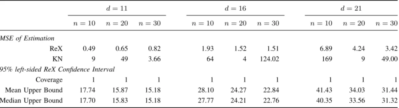
In this case, we set p = 8000, n to be from {10,20,30}, anddto be from{11,16,21}as in Section V-A. We setσto be(n/p)1/4 as discussed in Section IV, setµto be a regular sequence of lengthpfrom−5to5, and setτ to be2.Table II shows the results based on 1000 simulated datasets.
On the estimation, Table II shows again the problem of PCA based methods whenpis much larger thann: the KN method returns n−2 for seven out of nine scenarios. When n= 30 andd= 11ord= 16, the KN method returns better estimates, but its MSE is larger than that of the ReX estimation. Note that in these two scenarios for the KN method as well as in all nine scenarios for the ReX method, the MSEs are much smaller than those in Table I. One possible reason here is the standardization process. For the ReX method, recall from Section IV-A that the distribution of the estimators can be right-skewed. Since the variance estimation from the sample usually underestimatesτ2+σ2, the row maximumKp,dfrom standardized data can often be larger than that in the noiseless case, leading to a larger estimate ofdwhich offsets the right-skewness in the distribution.
On the ReX confidence intervals, Table II shows that the coverage probability of them is 1 for all nine scenarios. Although the coverage probability is conservative, the lengths of intervals are reasonably tight. Also, the median upper bounds are usually less than the mean ones, showing again the right-skewness. The problem of right-skewness is much more benign though.
In summary, in our simulation studies whenpis much larger than n, the traditional PCA based methods such as the KN method (1) may have a large MSE in estimatingd, (2) may not be able to provide confidence intervals ford, and (3) requires matrix-wise calculation. On the other hand, the ReX inference (1) has a small MSE in estimation, (2) provides confidence interval statements ford, and (3) only needs to scan through the row maxima in the matrix and is thus fast. These results demonstrate the advantages of using the ReX method for the detection of a low-rank structure in high dimensions with a small sample size.
TABLE I
PERFORMANCE OFREXINFERENCE FOR DIFFERENTn’S ANDd’S WHENp= 8000IN THE UNIT VARIANCE AND NOISELESS CASE.
d= 11 d= 16 d= 21
n= 10 n= 20 n= 30 n= 10 n= 20 n= 30 n= 10 n= 20 n= 30
MSE of Estimation
ReX 12.40 3.97 2.91 38.07 12.69 8.73 73.52 47.21 22.03
KN 9.00 49.00 148.16 64.00 4.00 143.98 169.00 9.00 49.00
95% left-sided ReX Confidence Interval
Coverage 0.958 0.946 0.944 0.951 0.949 0.950 0.926 0.937 0.952
Mean Upper Bound 18.21 15.15 14.20 31.41 23.66 22.13 49.32 35.74 31.01
Median Upper Bound 16.55 14.65 13.87 26.27 22.34 21.48 38.11 31.38 29.30
TABLE II
PERFORMANCE OFREXINFERENCE FOR DIFFERENTn’S ANDd’S WHENp= 8000IN THE EQUAL VARIANCE WITH NOISE CASE.
d= 11 d= 16 d= 21
n= 10 n= 20 n= 30 n= 10 n= 20 n= 30 n= 10 n= 20 n= 30
MSE of Estimation
ReX 0.49 0.65 0.82 1.93 1.52 1.51 6.89 4.24 3.42
KN 9 49 3.66 64 4 124.02 169 9 49.00
95% left-sided ReX Confidence Interval
Coverage 1 1 1 1 1 1 1 1 1
Mean Upper Bound 17.74 15.87 15.18 28.10 24.27 22.84 41.43 34.03 31.44
Median Upper Bound 17.70 15.83 15.18 27.77 24.21 22.76 40.35 33.56 31.32
increases. This problem could be related to the approximation error in (IV.3). Also, the ReX inference are based on solutions of (IV.5) and (IV.7). Such equations may not have a solution in difficult practical situations (This happens about 1% of the time whenn= 10andd= 21). Although this problem seems to disappear when nis above 10, a more stable algorithm is needed. We shall improve our method in these directions in future work.
VI. DISCUSSIONS
We develop a probabilistic upper bound for the maximal inner product between any set of unit vectors and a stochasti-cally independent uniformly distributed unit vector, as well as the limiting distributions of the maximal inner product when the set of unit vectors are i.i.d. uniformly distributed. We demonstrate the applications of these results the problems of spurious correlations and low-rank detections.
We emphasize that we focus our asymptotic theory in the uniform-n-large-pparadigm. This type of asymptotics is mo-tivated by the high-dimensional-low-sample-size framework [45] which is emerging in many areas of science. The proposed packing approach can be especially useful in this framework because (1) finite-sample properties can be studied, and (2) existing packing literature can be applied. In the future, we will continue to explore this type of asymptotics in more general situations. For the theory, we plan to investigate the distribution of the maximal inner products with more generally correlated Lj’s. One of the applications of the new theory could be a more accurate detection method of a low rank. We
also plan to improve and generalize the ReX detection method in the case whenτj’s are different, as well as in the case when the data are not Gaussian distributed.
APPENDIXA TECHNICALLEMMAS
We provide some key proofs in the appendix. Proofs of other results are immediate corollaries of these results. We start with the key observation that the distribution of each |hLj,Ui|2 is Beta(1/2,(n−1)/2), as discussed at the beginning in Section II-A and also in [44]. Based on this fact, we first derive a lemma on the tail bounds of theBeta(1/2,(n−1)/2) distribution. This lemma is proved by integration by parts, and the details are omitted.
Lemma A.1. For 0< w≤1, we have the following bounds for an incomplete beta integral:
2((n+ 2)w−1) (n2−1) w
−3/2(1−w)n−1 2
≤ Z 1
w
s−12(1−s)
n−3 2 ds
≤ 2
(n−1)w
−1/2(1−w)n−21
(A.1)
We also find a lemma on the uniform convergence of the function(n−1)(p2/(n−1)−1). This lemma is important for
Lemma A.2. Uniformly for any n ≥ 2, as p → ∞, (n−
1)(p2/(n−1)−1)→ ∞.
We derive below a lemma summarizing the uniform conver-gence of standardizing constants in the theorems. Their proofs are routine analysis and are omitted.
Lemma A.3. Consider the sequences ap,n = 1 −
p−2/(n−1)cp,n, bp,n = n−21p−2/(n−1)cp,n in Theorem II.4 where cp,n = n−21B 12,n−21
p
1−p−2/(n−1)2/(n−1) is a correction factor. For any fixed x, let wp,n = ap,n+bp,nx. We have the following asymptotic results:
1) Uniformly for any n ≥ 2, as p → ∞, cp,n/ n−21B 12,n−21
2/(n−1)
→ 1, bp,n → 0,
ap,n
1−p−2/(n−1) →1, and
bp,n
ap,n →0.
2) Uniformly for anyn≥2, asp→ ∞, (n+1)wp,n
(n+2)wp,n−1I x≤
n−1 2
+I x > n−1 2
→1.
APPENDIXB PROOFS INSECTIONII
Proof of Theorem II.1. To show (II.1), note that for δ ≥
1/(p2/(n−1)−1),(1 +δ)(1−p−2/(n−1))≥1,thus the bound
is trivial. Therefore, it is enough to show the convergence for any δ that 0 < δ <1/(p2/(n−1)−1). Similarly as the proof
of Theorem 6.3 in [50], by Lemma A.1 and the inequalities that Γ(x+ 1/2)/Γ(x)<√xas in [51], we have
P
max
j |hLj,Ui|> q
(1 +δ)(1−p−2/(n−1))
≤ pP
|hLj,Ui|> q
(1 +δ)(1−p−2/(n−1))
≤p
s 2 (n−1)π
(1−(1 +δ)(1−p−2/(n−1)))(n−1)/2
p
(1 +δ)(1−p−2/(n−1))
= s
2
π(1 +δ)
p1/(n−1)
1−δ(p2/(n−1)−1) (n−1)/2
p
(n−1)(p2/(n−1)−1)
≤
s 2
π(1 +δ)
p1/(n−1)exp
−1
2δ(n−1)(p
2/(n−1)−1)
p
(n−1)(p2/(n−1)−1)
(B.1)
Thus, by Lemma A.2,
P
max
j |hLj,Ui|>
q
(1 +δ)(1−p−2/(n−1))
→0
(B.2) as p→ ∞regardless ofn.
To see (II.3), note that if limp→∞n/logp=β > 0, then
p1/(n−1)→e1/β<∞.Thus we may set δ= 0to get (II.3). Also, if n → ∞ but n/logp → 0, then (B.1) is further bounded byqπ(n2−1)(1 +o(1)).Thus we have (II.3).
Proof of Theorem II.3. Since we already have the upper bound, it is enough to show that for any fixed δ such that 0< δ <1/2,
P
max
j |hLj,Ui|<
q
(1−δ)(1−p−2/(n−1))
→0.
(B.3)
By the independence discussed at the beginning of Sec-tion II-B, we have that forp→ ∞,
P
max
j |hLj,Ui|< q
(1−δ)(1−p−2/(n−1))
=
P
|hLj,Ui|< q
(1−δ)(1−p−2/(n−1))
p
≤ exp
−pP
|hLj,Ui|> q
(1−δ)(1−p−2/(n−1))
.
(B.4)
We will lower-bound the absolute value of the exponent in (B.4). By the lower bound in Lemma A.1 and the inequality that Γ(x+ 1)/Γ(x+ 1/2)>px+ 1/4 as in [51], we have
pP
|hLj,Ui|> q
(1−δ)(1−p−2/(n−1))
= p
B 1/2,(n−1)/2 Z 1
(1−δ)(1−p−2/(n−1))
x−1/2(1−x)(n−3)/2dx
≥
s 1
π(1−δ)3
√
2n−3
n2−1
p1/(n−1)
p
(p2/(n−1)−1)3·
1 +δ(p2/(n−1)−1)(n−1)/2
(1−δ)n(p2/(n−1)−1)−1
≥
s 2
π(1−δ)
p1/(n−1) 1 +δ(p2/(n−1)−1)(n−1)/2
p
n(p2/(n−1)−1) (1 +o(1)).
(B.5)
In the last step of (B.5), we use Lemma A.2 again. It is now easy to see that
pP
|hLj,Ui|>
q
(1−δ)(1−p−2/(n−1))
→ ∞ (B.6)
asp→ ∞regardless of the rate ofn=n(p), which completes the proof of Theorem II.3.
Proof of Theorem II.4. Ifx≥(n−1)/2,thenap,n+bp,nx≥1 and the result is trivial. For x < (n−1)/2, by Lemma A.1 and Lemma A.3, uniformly for anyn≥2, asp→ ∞,
−logP
M2
p,n−ap,n
bp,n
< x
=−log{P(|hLj,Ui|2< bp,nx+ap,n)p} = 2p(1−ap,n−bp,nx)
(n−1)/2 B 1
2,
n−1 2
(n−1)p
ap,n+bp,nx
(1 +o(1))
=2p 1−1 +cp,np −2 (n−1) − 2
n−1cp,np −2 (n−1)x
(n−1) 2
B 1 2,
n−1 2
(n−1)pap,n(1 +o(1)) (1 +o(1))
= 1− 2
n−1x (n−1)/2
(1 +o(1)).
(B.7)
Whenn→ ∞, 1− 2
n−1x
(n−1)/2
APPENDIXC PROOFS INSECTIONIII
Proof of Theorem III.1. It is easy to show (III.3) and (III.4). To show (III.5), note that for any0< ε <1,
P
kXk∞/ q
d(1−p−2/(d−1))>1
=P
kZk2max
j |hLj,Ui|/ q
d(1−p−2/(d−1))>1
≤P
max
j |hLj,Ui|> q
(1−ε)(1−p−2/(d−1))
+P
kZk2>
p (1 +ε)d
(C.1)
We will show each of the two summands in the last line can be made small with a proper choice of ε=ε(p).
By the proof of Theorem II.1, we see that
P
max
j |hLj,Ui|>
q
(1−ε)(1−p−2/(d−1))
≤ s
2
π(1−ε)
p1/(d−1)exp
1
2ε(d−1)(p
2/(d−1)−1)
p
(d−1)(p2/(d−1)−1)
(C.2)
Note also that kZk2
2 ∼χ2d. Thus by the Chernoff bound for
χ2
d distribution,
P kZk2> p
(1 +ε)d
=P kZk2
2>(1 +ε)d
≤((1 +ε)e−ε)d/2
≤e−dε2/6
(C.3)
Due to (C.2) and (C.3), we letε=ε(p) = log logp/(4 logp).
In the case when limp→∞(log logp)
2d
(logp)2 → ∞, both (C.2) and
(C.3) converge to 0.
Proof of Theorem III.3. Note that,
Kp,d−udap,d=Mp,d2 (kZk
2
2−ud) +ud(Mp,d2 −ap,d) (C.4) Now note also that ap,d is bounded and that Mp,d/ap,d
prob.
−→
1.Therefore, the theorem follows from Slutsky’s theorem by checking the limit of the ratio vdap,d andudbp,d and picking the one with a larger magnitude as the scaling factor.
ACKNOWLEDGMENT
The author appreciates the insightful suggestions from L. D. Brown, A. Buja, T. Cai, J. Fan, J. S. Marron, and H. Shen. The author thanks R. Adler, J. Berger, R. Berk, A. Budhiraja, E. Candes, L. de Haan, J. Galambos, E. George, S. Gong, J. Hannig, T. Jiang, I. Johnstone, A. Krieger, R. Lead-better, R. Li, D. Lin, H. Liu, J. Liu, W. Liu, Y. Liu, Z. Ma, X. Meng, A. Munk, A. Nobel, E. Pitkin, S. Provan, A. Rakhlin, D. Small, R. Song, J. Xie, M. Yuan, D. Zeng, C.-H. Zhang, N. Zhang, L. Zhao, Y. Zhao, and Z. Zhao for helpful dis-cussions. The author also thanks the editors and reviewers for important comments that substantially improve the manuscript.
The author is particularly grateful for L. A. Shepp for his inspiring introduction of the random packing literature.
This research is partially supported by NSF DMS-1309619, NSF DMS-1613112, NSF IIS-1633212, and the Junior Faculty Development Award at UNC Chapel Hill. This material was also partially based upon work supported by the NSF under Grant DMS-1127914 to the Statistical and Applied Mathemat-ical Sciences Institute. Any opinions, findings, and conclusions or recommendations expressed in this material are those of the author(s) and do not necessarily reflect the views of the National Science Foundation.
REFERENCES
[1] J. Fan, F. Han, and H. Liu, “Challenges of big data analysis,” National Science Review, vol. 1, pp. 293–314, 2014.
[2] I. M. Johnstone and D. M. Titterington, “Statistical challenges of high-dimensional data,”
Philosophical Transactions of the Royal Society A: Mathematical, Physical and Engineering Sciences, vol. 367, no. 1906, pp. 4237–4253, 2009. [Online]. Available: http://rsta.royalsocietypublishing.org/content/ 367/1906/4237.abstract
[3] J. Fan, J. Lv, and L. Qi, “Sparse high dimensional models in economics,” Annual review of economics, vol. 3, p. 291, 2011.
[4] J. Fan, S. Guo, and N. Hao, “Variance estimation using refitted cross-validation in ultrahigh dimensional regres-sion,” J. R. Statist. Soc. B, vol. 74, pp. 37–65, 2012. [5] I. Markovsky,Low-Rank Approximation: Algorithms,
Im-plementation, Applications. New York: Springer, 2012. [6] B. Yang, “Projection approximation subspace tracking,”
Signal Processing, IEEE Transactions on, vol. 43, no. 1, pp. 95–107, Jan 1995.
[7] D. J. Rabideau, “Fast, rank adaptive subspace tracking and applications,”Signal Processing, IEEE Transactions on, vol. 44, no. 9, pp. 2229–2244, 1996.
[8] A. Kav˘ci´c and B. Yang, “Adaptive rank estimation for spherical subspace trackers,” Signal Processing, IEEE Transactions on, vol. 44, no. 6, pp. 1573–1579, Jun 1996. [9] E. C. Real, D. W. Tufts, and J. W. Cooley, “Two algo-rithms for fast approximate subspace tracking,” Signal Processing, IEEE Transactions on, vol. 47, no. 7, pp. 1936–1945, 1999.
[10] M. Shi, Y. Bar-Ness, and W. Su, “Adaptive estimation of the number of transmit antennas,” inMilitary Communi-cations Conference, 2007. MILCOM 2007. IEEE. IEEE, 2007, pp. 1–5.
[11] R. Badeau, G. Richard, and B. David, “Fast and stable yast algorithm for principal and minor subspace track-ing,” Signal Processing, IEEE Transactions on, vol. 56, no. 8, pp. 3437–3446, 2008.
[12] S. Bartelmaos and K. Abed-Meraim, “Fast principal component extraction using givens rotations,” Signal Processing Letters, IEEE, vol. 15, pp. 369–372, 2008. [13] X. G. Doukopoulos and G. V. Moustakides, “Fast and
[14] S. Kritchman and B. Nadler, “Determining the number of components in a factor model from limited noisy data,” Chemometrics and Intelligent Laboratory Systems, vol. 94, no. 1, pp. 19 – 32, 2008. [Online]. Available: http://www.sciencedirect.com/science/article/ pii/S0169743908001111
[15] ——, “Non-parametric detection of the number of sig-nals: Hypothesis testing and random matrix theory,”
Signal Processing, IEEE Transactions on, vol. 57, no. 10, pp. 3930–3941, Oct 2009.
[16] I. M. Johnstone and A. Y. Lu, “On consistency and sparsity for principal components analysis in high dimen-sions,” Journal of the American Statistical Association, vol. 104, no. 486, 2009.
[17] P. Perry and P. Wolfe, “Minimax rank estimation for subspace tracking,”Selected Topics in Signal Processing, IEEE Journal of, vol. 4, no. 3, pp. 504–513, June 2010. [18] Q. Berthet and P. Rigollet, “Optimal detection of sparse principal components in high dimension,” The Annals of Statistics, vol. 41, no. 4, pp. 1780–1815, 08 2013. [Online]. Available: http://dx.doi.org/10.1214/ 13-AOS1127
[19] D. L. Donoho and M. Gavish, “The optimal hard thresh-old for singular values is 4/sqrt (3),” arXiv preprint arXiv:1305.5870, 2013.
[20] T. Cai, Z. Ma, and Y. Wu, “Optimal estimation and rank detection for sparse spiked covariance matrices,” Probability Theory and Related Fields, pp. 1–35, 2014. [Online]. Available: http://dx.doi.org/10. 1007/s00440-014-0562-z
[21] Y. Choi, J. Taylor, and R. Tibshirani, “Selecting the number of principal components: estimation of the true rank of a noisy matrix,”arXiv preprint arXiv:1410.8260, 2014.
[22] R. A. Rankin, “The closest packing of spherical caps in n dimensions,” Proceedings of the Glasgow Mathematical Association, vol. 2, pp. 139–144, 7 1955. [Online]. Available: http://journals.cambridge.org/ article S2040618500033219
[23] T. M. Thompson,From Error-correcting Codes through Sphere Packings to Simple Groups. Mathematical Association of America, 1983.
[24] J. H. Conway, N. J. A. Sloane, and E. Bannai, Sphere-packings, Lattices, and Groups. New York, NY, USA: Springer-Verlag New York, Inc., 1987.
[25] D. Hilbert, “Mathematical problems,” Bulletin of the American Mathematical Society, vol. 8, no. 10, pp. 437– 479, 1902.
[26] A. D. Wyner, “Random packings and coverings of the unit n-sphere,” Bell System Technical Journal, vol. 46, pp. 2111–2118, 1967.
[27] A. Barg and D. Nogin, “Bounds on packings of spheres in the grassmann manifold,” Information Theory, IEEE Transactions on, vol. 48, no. 9, pp. 2450–2454, Sep 2002. [28] K. K. Mukkavilli, A. Sabharwal, E. Erkip, and B. Aazhang, “On beamforming with finite rate feedback in multiple-antenna systems,”Information Theory, IEEE Transactions on, vol. 49, no. 10, pp. 2562–2579, 2003.
[29] O. Henkel, “Sphere-packing bounds in the grassmann and stiefel manifolds,”IEEE Transactions on Information Theory, vol. 51, no. 10, pp. 3445–3456, 2005.
[30] R. Koetter and F. R. Kschischang, “Coding for errors and erasures in random network coding,”Information Theory, IEEE Transactions on, vol. 54, no. 8, pp. 3579–3591, 2008.
[31] W. Dai, Y. Liu, and B. Rider, “Quantization bounds on grassmann manifolds and applications to mimo commu-nications,” Information Theory, IEEE Transactions on, vol. 54, no. 3, pp. 1108–1123, 2008.
[32] R.-A. Pitaval, H.-L. Maattanen, K. Schober, O. Tirkko-nen, and R. Wichman, “Beamforming codebooks for two transmit antenna systems based on optimum grassman-nian packings,” Information Theory, IEEE Transactions on, vol. 57, no. 10, pp. 6591–6602, 2011.
[33] M. Dalai, “Lower bounds on the probability of error for classical and classical-quantum channels,” Information Theory, IEEE Transactions on, vol. 59, no. 12, pp. 8027– 8056, Dec 2013.
[34] T. Hastie, R. Tibshirani, and J. Friedman,The Elements of Statistical Learning: Prediction, Inference and Data Mining, 2nd ed. Springer Verlag., 2009.
[35] P. B¨uhlmann and S. van de Geer, Statistics for High-Dimensional Data. Springer, 2011.
[36] M. R. Leadbetter, Extremes and Related Properties of Random Sequences and Processes. Springer-Verlag, 1983.
[37] L. de Haan and A. Ferreira, Extreme Value Theory: An Introduction. Springer, 2006.
[38] R. J. Adler, “An introduction to continuity, extrema, and related topics for general gaussian processes,” Lecture Notes-Monograph Series, pp. i–155, 1990.
[39] A. Hero and B. Rajaratnam, “Large-scale correlation screening,” Journal of the American Statistical Associ-ation, vol. 106, pp. 1540–1552, 2012.
[40] T. T. Cai and T. Jiang, “Limiting laws of coherence of random matrices with applications to testing covariance structure and construction of compressed sensing matri-ces,” Ann. Statist, vol. 39, pp. 1496–1525, 2011. [41] ——, “Phase transition in limiting distributions of
co-herence of high-dimensional random matrices,”J. Multi-variate Analysis, vol. 107, pp. 24–39, 2012.
[42] T. T. Cai, J. Fan, and T. Jiang, “Distribution of angles in random packing on spheres,” J. Machine Learning Research, vol. 14, pp. 1801–1828, 2013.
[43] J. Fan, Q.-M. Shao, and W.-X. Zhou, “Are discoveries spurious? distributions of maximum spurious correlations and their applications,”arXiv preprint arXiv:1502.04237, 2015.
[44] R. J. Muirhead, Aspects of Multivariate Statistical The-ory. Wiley, 1982.
[46] K.-T. Fang, S. Kotz, and K. W. Ng, Symmetric multi-variate and related distributions. Chapman and Hall, 1990.
[47] A. W. van der Vaart, Asymptotic Statistics. Cambridge University Press, Cambridge, 1998.
[48] M. S. Bartlett, “Properties of sufficiency and statistical tests,”Proceedings of the Royal Society of London. Series A, vol. 160, no. 901, pp. 268–282, 1937.
[49] H. Cohn and Y. Zhao, “Sphere packing bounds via spherical codes,”Duke Mathematical Journal, vol. 163, no. 10, pp. 1965–2002, 07 2014. [Online]. Available: http://dx.doi.org/10.1215/00127094-2738857
[50] R. Berk, L. Brown, A. Buja, K. Zhang, and L. Zhao, “Valid post-selection inference,”The Annals of Statistics, vol. 41, no. 2, pp. 802–837, 04 2013. [Online]. Available: http://dx.doi.org/10.1214/12-AOS1077
[51] G. J. O. Jameson, “Inequalities for gamma function ratios,”The American Mathematical Monthly, vol. 120, pp. 936–940, 2013.