s
s
THE ALLOCATION OF TALENT IN BRAZIL AND INDIA
ss
Kanat Abdulla
ss
A dissertation submitted to the faculty at the University of North Carolina at Chapel Hill in partial fulfillment of the requirements for the degree of Doctor of Philosophy in the
Department of Economics
ssss
Chapel Hill 2018
ss
ssssssssssssssssssssssssssssssssssssssssssssssssssssssssssssssssssssssssssssApproved by:
ssssssssssssssssssssssssssssssssssssssssssssssssssssssssssssssssssssssssssssLutz Hendricks
ssssssssssssssssssssssssssssssssssssssssssssssssssssssssssssssssssssssssssssSimon Alder
ssssssssssssssssssssssssssssssssssssssssssssssssssssssssssssssssssssssssssssLuca Flabbi
ssssssssssssssssssssssssssssssssssssssssssssssssssssssssssssssssssssssssssssKlara Peter
ssssssssssssssssssssssssssssssssssssssssssssssssssssssssssssssssssssssssssssToan Phan
s s s s s s s s s s s s s s s s s s s
s s
s
ABSTRACT
Kanat Abdulla: The Allocation of Talent in Brazil and India (Under the direction of Lutz Hendricks)
ss
This dissertation is a collection of two independent essays on human capital in
developing countries. In the first chapter, I investigate the labor market outcomes in
Brazil and India and examine the effect of the frictions in the human capital accumulation
and in the labor market on the aggregate output in these countries. The second chapter
tests theories related to immigrant characteristics and their earnings by investigating
s
ACKNOWLEDGEMENTS
I would like to express my gratitude to my advisor, Lutz Hendricks, for the
con-tinuous support throughout the research, for his motivation and immense expertise that
greatly assisted the research. I am also grateful to Simon Alder, Luca Flabbi, Klara Peter,
and Toan Phan for their valuable suggestions and comments that helped me improve the
TABLE OF CONTENTS
LIST OF TABLES . . . vii
LIST OF FIGURES . . . ix
1 THE ALLOCATION OF TALENT IN BRAZIL AND INDIA . . . 1
1.1 Introduction . . . 1
1.2 Literature review . . . 3
1.3 Data . . . 4
1.3.1 Data from Brazilian household survey . . . 6
1.3.2 Data from Indian household survey . . . 7
1.3.3 Home sector and sample selection . . . 8
1.4 The Model . . . 11
1.4.1 Household Problem . . . 12
1.4.2 Firm problem . . . 14
1.4.3 Market clearing . . . 15
1.4.4 General equilibrium . . . 15
1.5 Empirical findings . . . 16
1.5.1 Occupational distribution across groups . . . 16
1.5.2 Wage gap estimations . . . 19
1.5.3 Estimation of Frictions . . . 22
1.6 Results . . . 25
1.6.1 Model fit . . . 26
1.6.2 Output gain . . . 28
1.6.3 Robustness analysis . . . 34
2 IMMIGRANT CHARACTERISTICS IN LOW-INCOME COUNTRIES . . 40
2.1 Introduction . . . 40
2.2 Literature review . . . 43
2.2.1 Immigrant earnings and human capital . . . 44
2.2.2 Skill transferability . . . 45
2.2.3 Assimilation . . . 46
2.3 Data . . . 48
2.4 Human capital vs skill transferability . . . 53
2.5 Selection . . . 55
2.6 Unobserved skill differences . . . 59
2.7 Assimilation . . . 62
2.7.1 Human capital investment model . . . 63
2.7.2 Empirical analysis . . . 63
2.7.3 Occupational distribution and mobility of immigrants . . . 67
2.8 Conclusion . . . 72
LIST OF TABLES
1.1 Sample statistics (Brazilian survey) . . . 7
1.2 Sample statistics (Indian survey) . . . 8
1.3 Sample data . . . 9
1.4 Occupational similarity index . . . 19
1.5 Conditional log difference in wages . . . 21
1.6 Relationship of wage gaps and propensities . . . 22
1.7 Baseline parameter values . . . 23
1.8 Summary stats of frictions across countries . . . 25
1.9 Occupational shares in Brazil and India (data vs model) . . . 27
1.10 Mean earnings across groups in Brazil and India (data vs model) . . . 28
1.11 Counterfactuals: Output gain in Brazil . . . 30
1.12 Counterfactuals: Output gain in India . . . 31
1.13 Counterfactuals: Output gain in India with detailed caste categories . . . 32
1.14 Counterfactual output growth in India . . . 34
1.15 Output gain in Brazil due to removed frictions . . . 35
1.16 Output gain in India due to removed frictions . . . 36
2.1 Sample data . . . 49
2.2 IPUMS Educational attainment . . . 50
2.3 Sample data . . . 52
A1 Occupational coding . . . 77
A2 Broader occupational categories . . . 78
A3 Summary statistics . . . 79
A4 Share of college-educated . . . 80
A5 Activity status . . . 81
A7 Regression results for India . . . 82
A8 Occupational categories . . . 83
LIST OF FIGURES
1.1 Share of groups in highly skilled occupations . . . 17
2.1 The share of college-educated workers in high-skilled occupations . . . 55
2.2 Education levels of immigrants vs non-migrants . . . 58
2.3 Earnings gap of immigrants relative to natives . . . 61
2.4 Assimilation of immigrants in the US . . . 65
2.5 Assimilation of immigrants in Brazil . . . 66
2.6 Occupational distribution of immigrants . . . 69
Chapter 1
THE ALLOCATION OF TALENT IN BRAZIL AND INDIA
1.1 Introduction
Hsieh et al. (2013) ask whether improved allocation of workers according to their
talents was an important source of productivity growth in the U.S. This is motivated by
substantial differences in occupational choices between men/women and blacks/whites.
In particular, they document that the share of women and blacks in high-skill occupations
was very low relative to that of white men. These differences in occupational distribution
of women and blacks relative to white men declined over time, suggesting that
misal-location has diminished. This change has positively affected the aggregate productivity
growth in the United States. Hsieh et al. (2013) argue that better allocation of talent
explains 15–20% of the economic growth in the U.S.
I use micro-level survey data from Brazil and India with detailed information on
socio-economic and occupational characteristics and their earnings to investigate the role
of allocation of talent in economic development of these countries. The analysis in these
countries is motivated by the fact that there are substantial fractions of the population
that are disadvantaged in terms of access to quality education and jobs. As a result there
are large differences in occupational distribution and earnings between groups. This paper
will argue that the allocation of talent affects the aggregate output in these countries.
Allocation of talent refers to the distribution of various groups across occupations,
where the groups are categorized by race1 and gender. Talent is misallocated when there
is a difference in the occupational distribution between the groups. The main forces
that produce the difference in occupational distribution across groups are frictions in
accumulation of human capital and frictions in labor market. Frictions are estimated from
the observed occupational distributions and the wage gap between groups. Given these
frictions, workers choose occupations where they have the highest utility. An augmented
Roy model of occupational choice developed by Hsieh et al. (2013) allows me to determine
the potential gains to output from decreasing frictions in Brazil and India.
I investigate the occupational distribution and wage gaps of four groups (white men,
white women, brown men and brown women) in Brazil and four groups (other men, other
women, scheduled caste/tribe men, scheduled caste/tribe women) in India. The term
“brown” is used to refer to Brazilians of mixed ethnic ancestries and sometimes known
as “parda” in the Brazilian censuses. Browns make up 43% of the Brazilian population.
Scheduled caste and tribe are terms recognized by the Indian constitution and refer to
the most disadvantaged groups in India. They consist of 26% of the country’s population.
I show that frictions are substantial, especially for brown women in Brazil and
scheduled caste women in India. I conduct a counterfactual experiment which helps me to
assess the role of misallocation of talent in productivity in these countries. First, I reduce
frictions faced by the groups by half. I find that reducing frictions faced by various groups
in Brazil and India by half increases the aggregate productivity by 10–20% in Brazil and
by 14–22% in India. Second, I investigate the gain after eliminating frictions in these
countries. Removing frictions increases the aggregate productivity of the countries by
21–42% in Brazil and by 36–46% in India.
This paper is organized as follows: Section 1.2 reviews the literature, Section 1.3
describes the census data obtained from the Integrated Public Use Microdata Series,
Section 1.4 discusses the model, Section 1.5 provides an empirical evidence on earnings
of various groups and their occupational distribution, Section 1.6 describes the results of
1.2 Literature review
In most countries there are disadvantaged groups within population. They are
disadvantaged because they face discrimination in the early stages of acquisition of human
capital or later face unequal access to jobs or both. Brazil and India are among those
countries.
There is significant evidence that in Brazil there is a gap in earnings between men
and women and race groups. Men in Brazil earn about 25% more and are more likely to
participate in the labor force than women in Brazil (Arabsheibani et al. (2003)). White
people in Brazil earn 26% more than brown people with same human capital and labor
market characteristics (Telles (2006)). A significant part of the racial wage gap in Brazil
occurs because of discrimination (Lovell (1993)). The analysis of the returns to schooling
for various groups shows that the returns to schooling for whites are higher than the
returns to schooling for dark-skinned population (Loureiro et al. (2004)). The difference
in occupational distribution between men and women in Brazil has an effect on wage gap
between these groups (Madalozzo R. (2010)).
Caste- and gender-based discrimination in India produces significant gaps in terms
of earnings and labor market participation. Scheduled caste and scheduled tribe workers
earn 30% less than equally qualified others (Madheswaran and Attewell (2007)). The
unconditional earnings gap of women relative to men in India was 55% in 1999–2000 and
49% in 2009–2010, and the gap persists even within the same education level and within
most occupations and industries (Deshpande et al. (2018)). Occupational
discrimina-tion is more prevalent than wage discriminadiscrimina-tion. Some castes are discriminated against
in terms of unequal access to jobs, especially in the private sector (Madheswaran and
Attewell (2007)). Discrimination in hiring processes is a common practice in the urban
labor market in India (Thorat and Attewell (2007)).
cer-tain groups out of occupations for which they have necessary skills. This is called talent
misallocation. Whether or not this misallocation has an effect on overall productivity has
been the focus of a number of studies that have contributed to the understanding of the
role of talent misallocation in economic development. One of the important factors in
the allocation of talent is the relative rewards that different professions receive (Acemoglu
(1995)). Rewards for entrepreneurship determine the allocation of productive versus
un-productive entrepreneurship labor, which affects the aggregate output (Baumol (1990)).
By analyzing the occupational distribution of women and blacks relative to white men in
the period from 1960 to 2008, Hsieh et al. (2013) find that the share of women and blacks
in high-skill occupations was very low relative to that of white men in the 1960s. This
occupational gap shrank over time, affecting aggregate productivity growth in the United
States. In particular, Hsieh et al. (2013) argue that better allocation of talent explains
15–20% of the economic growth in the U.S.
1.3 Data
I use Brazilian and Indian survey data available at Integrated Public Use Microdata
Series (IPUMS). The Brazilian data spans the 1991, 2000, and 2010 survey years with
a total sample size of about 5–10 million individuals per survey year. Indian data is a
socio-economic survey conducted by the National Sample Survey Organization of India
every 5–6 years with a sample size of 500–600 thousand individuals. The variable names,
coding schemes, and documentation are consistent for most samples.
The analysis uses a variable from IPUMS that indicates an individual’s primary
occupation, which is classified according to the system used by the respective census of
countries. Brazilian and Indian surveys have different classification systems for
occupa-tions. Moreover, the Brazilian survey has varying classifications for different periods. To
make data comparable across years and countries, I harmonize occupational coding to the
to 66 occupations.2 Some related occupation categories were merged into one sub-heading.
For instance, management-related occupations include some administrative support
occu-pations, and the computer and communications equipment operator occupation consists of
communication equipment operators and computer and peripheral equipment operators.
Other key variables used in the analysis are variables indicating an individual’s
earnings, hours worked, employment status, education, and race. For individual’s earnings
I use a variable that represents the total income from the labor (from wages, a business,
or a farm) in the previous month or year.3 A variable that indicates individual’s social
group or race in Brazilian census is named as “race” and in Indian census as “social group”.
Employment status of the person is defined by Emptat, which I use to identify employed
individuals. Hrswork4 shows a person’s hours worked per week, and wkswork4 shows
person’s weeks worked per year, which are used to compute hourly wages. A person’s
educational attainment is identified by the variable “edattaind” and shows the person’s
educational attainment in terms of the level of schooling completed, i.e. a person attending
the final year of college receives the code for having completed secondary degree only.
From this variable I construct a variable that indicates a person’s number of schooling
years completed, “educ”. There is a limitation in constructing years of schooling from
edattaind because it will show only the approximate number of years of schooling. For
example, there is a discontinuity between 8 and 12 years of schooling, and it will not allow
me to identify individuals with more than 16 years of schooling.
From the available data I construct hourly wages and experience. Hourly wages are
constructed from income, weeks worked per year and hours worked per week.
Experi-ence is constructed from individual’s age and years of schooling completed as age minus
schooling minus 6. As I discussed previously, there is a problem in the recording years of
2The detailed occupational coding is provided in Appendix.
3The variable available in IPUMS for Brazil and India is called “incearn”. I also use data from the
US in analysis. For the US sample I use “incbus”, income from business, “incwage”, wage income, and “incfarm”, income from farming.
schooling correctly for some observations, which leads to difficulty in recording the
poten-tial experience for some observations. It may overstate the actual potenpoten-tial experience if
actual years of schooling is higher and understate if the actual years of schooling is lower.
Summary statistics for key variables used in the analysis are provided in Appendix
Table A3.
1.3.1 Data from Brazilian household survey
The data are analyzed for the following sample periods: 1991, 2000, and 2010. The
following restrictions are made to the data: 1) only brown5 and white are chosen out of
5 possible race groups, 2) the analysis is restricted to individuals whose ages are between
25 and 60, 3) individuals who are on active military duty and unemployed individuals are
excluded, 4) individuals who are unable to work due to disability, retired or at school are
also excluded from the sample.
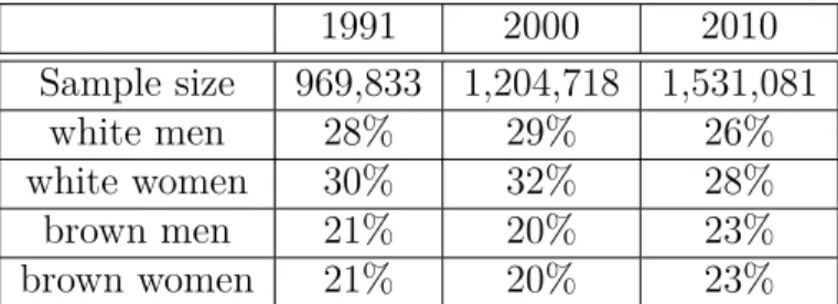
Table 1.1 reports the summary statistics of the restricted sample across years. The
number of observations, as shown in the table, has increased considerably over time, with
the sample size increasing two-fold from 969,000 observations to 1,530,000 observations
over the 20-year period. The largest share of the sample belong to whites: the share of
whites was 59% in 1991 and 55% in 2010. The shares of race groups have not changed
much over the course of the period. White males and females constituted 28% and 30%
of the population and 26% and 28% of the population in 1991 and 2010, respectively.
The proportions of brown men and brown females have slightly increased from 21% to
23%, respectively, over the period. The education levels of these population have changed
significantly over the 20-year period. Table A4 in Appendix reports the share of
college-educated individuals by groups and survey years. In 1991 the share of college-college-educated
individuals was only 5.5% of the total population, but in 2010 it had increased to 10.4%.
5In the analysis I use only brown and white because these races constitute the largest share of the
Among the race groups, brown men had the fewest college-educated individuals: in 1991
the share of college-educated brown men was only 1.8% of the total brown men, in 2010 it
had increased only to 3.8%. White women in the sample show the highest increase in the
share of college-educated individuals. In the total population the share of college-educated
white women was 7.7% in 1991; by 2010 it had increased to 17.1%.
1991 2000 2010
Sample size 969,833 1,204,718 1,531,081
white men 28% 29% 26%
white women 30% 32% 28%
brown men 21% 20% 23%
brown women 21% 20% 23%
Table 1.1: Sample statistics (Brazilian survey)
1.3.2 Data from Indian household survey
For India, IPUMS provides consistent data for the following sample periods: 1993,
1999, and 2004. There is a lack of data comparability across different survey periods in
regard to caste identities. In the 1999 and 2004 surveys, other backward castes are treated
separately; however prior to 1999 other backward castes and others were treated as one
group. For the purposes of comparability across different periods, I treat other backward
castes and others as one group in the 1999 and 2004 sample periods.
The following restrictions are made to the data: 1) the analysis is restricted to
individuals aged 25–60, 2) individuals who are on active military duty and unemployed
individuals are excluded, 3) individuals who are unable to work due to disability, retired,
or at school are also excluded from the sample.
There are four main caste classifications: scheduled caste, scheduled tribe, other
backward castes, and others. The most disadvantaged castes in socio-economic terms
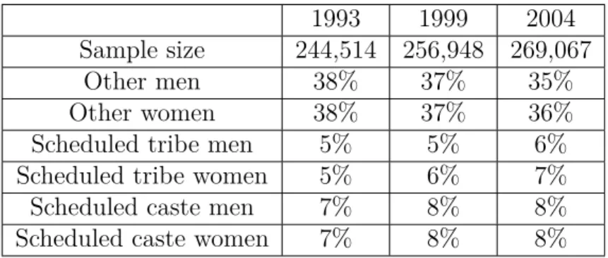
are scheduled castes and scheduled tribes. Table 1.2 reports the summary statistics of
the samples. The sample size does not change much across periods: 244,514, 256,948 and
sample are “others” with 72–75% of the total population. Scheduled tribes and scheduled
castes are minority groups of the Indian population. They respectively comprise 13%
and 16% of India’s total population in the sample. The share of castes did not show
appreciable change over time.
The majority of the Indian working population have education levels less than college
degree. As shown in Table A4, only 6.8% and 7.8% of the total population had a college
degree in 1999 and 2004, respectively. There is diversity in terms of education attainment
among gender and castes. While 11.5% of other men had a college degree in 1999, the
share of college-educated other women was only 5.5%. This is also true for other castes.
Only 1.2 and 0.5% of scheduled tribe and scheduled caste women had college degrees in
1991 as compared to 3.5% and 2.5% of men from respective castes. We see an increase in
college attainment for all castes. Overtime the groups experienced increase in the share
of college-educated individuals. In particular, scheduled tribe and scheduled caste men
show a noticeable increase in the share of college educated individuals, from 3.5% to 7%
and from 2.5% to 5.1%, respectively, in 1993 and 2004.
1993 1999 2004
Sample size 244,514 256,948 269,067
Other men 38% 37% 35%
Other women 38% 37% 36%
Scheduled tribe men 5% 5% 6%
Scheduled tribe women 5% 6% 7%
Scheduled caste men 7% 8% 8%
Scheduled caste women 7% 8% 8%
Table 1.2: Sample statistics (Indian survey)
1.3.3 Home sector and sample selection
A substantial part of the working population in developing countries is occupied
in the informal sector. Taking into account this sector will greatly influence the results.
IPUMS provides information about the employment status of individuals in the sample.
at school, or retired and living on rents. Table A5 in Appendix shows the observation
numbers in each category. The sample excludes individuals who are at school, unable to
work or retired. So individuals in labor force and individuals not in labor force but those
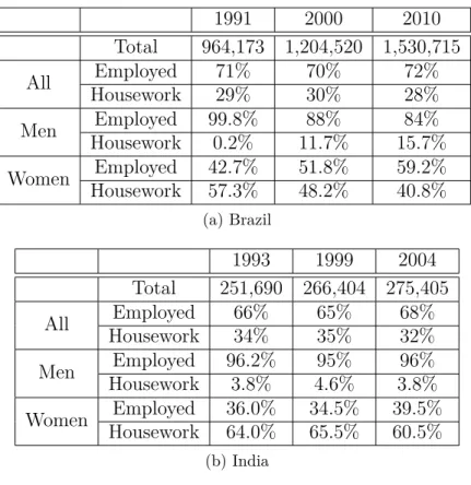
in housework are in the sample. As can be seen from Table 1.3, approximately 1/3 of
the working age population in Brazil and India are classified as employed in housework.
Most of the population occupied in housework in both countries are women: 40.8% of
women in Brazil in 2010 and 60.5% of women in India in 2004 were classified as working
in housework. For men this number is much lower: 15.7% in Brazil and 3.8% in India in
the corresponding years.
1991 2000 2010
Total 964,173 1,204,520 1,530,715
All Employed 71% 70% 72%
Housework 29% 30% 28%
Men Employed 99.8% 88% 84%
Housework 0.2% 11.7% 15.7%
Women Employed 42.7% 51.8% 59.2%
Housework 57.3% 48.2% 40.8%
(a) Brazil
1993 1999 2004
Total 251,690 266,404 275,405
All Employed 66% 65% 68%
Housework 34% 35% 32%
Men Employed 96.2% 95% 96%
Housework 3.8% 4.6% 3.8%
Women Employed 36.0% 34.5% 39.5%
Housework 64.0% 65.5% 60.5%
(b) India
Table 1.3: Sample data
In addition to the 66 occupation categories defined above, I create another
occu-pational category for the home sector. An individual who is not in the labor force is
considered to be working in the home sector. I impute wages for individuals in the home
same observed characteristics. The observed characteristics include the region where an
individual resides, the group to which individual belongs, schooling, and experience. Here
I assume that the relationship between earnings and these characteristics are the same
for the home and the market sectors.
Estimating the wage equation for individuals who are employed may not produce
similar results to estimating it for the population as a whole. Those who are employed are
the ones who made the decision to work, but this decision may not have been made
ran-domly. If the ones who choose to work tend to have higher (lower) wages than those not
in the labor force, then the sample of observed wages will be biased upward (downward).
Thus this produces a biased result when estimating the returns to observable
charac-teristics like education or experience. To assign wages to workers in the home sector, I
implement selection bias correction, following Heckman (1979).
Thus the following model is analyzed:
log(wage) =β1+β2group+β3educ+β4exp
+β5exp2+β6year+β7region+β8marst+ε1
(1.1)
and the earnings are observed if
γ1+γ2group+γ3educ+γ4exp+γ5exp2
+γ6year+γ7region+γ8marst+γ9numperson+ε2>0
(1.2)
I assume that Xi includes education and experience, dummy variables for groups,
census region, year, and marital status, and Zi includes variables in Xi plus the number
of people in the household.6 The model is estimated on women. Using the estimated
unbiased coefficients, I predict the earnings for women in the home sector.
6The studies use the number of children as an exclusion restriction (e.g. Mulligan and Rubinstein
1.4 The Model
I use an augmented Roy (1951) model presented by Hsieh et al. (2013). There are an
infinite number of individuals and a representative firm. Individuals consume goods, rent
labor to maximize their utilities, and choose occupation that deliver the highest utility.
A firm hires labor inputs and produces goods.
Demographics: There is a continuum of people, each belonging to a groupg based
on gender and race.
Preferences: Individuals maximize their utility:
Uig=cβig(1−sig) (1.3)
where i refers to occupation, cig is consumption, sig schooling, and β is a parameter
showing the tradeoff between consumption and leisure.
Endowments: At birth, individuals are endowed with a random skill i from a
extreme value distribution as in McFadden (1974) and Eaton and Kortum (2002).
Fg(1, ..., N) =exp{−[ N
X
i=1
(Tig−θi )]
1−ρ} (1.4)
whereθ determines the skill dispersion,ρ determines the correlation of skills across
occu-pations, andTig defines occupation-group specific ability.
Technology: An individual accumulates human capital from education s and
ex-pendituree according to the production function:
h(e, s) = ¯higsφigie η
ig (1.5)
The production function varies by group. The elasticity of human capital with
respect to schooling, φi, differs by occupation. The parameter ¯hig, efficiency in human
family background.
Markets: There is a market for labor rental.
1.4.1 Household Problem
Households maximize their utility by choosing consumption, schooling, and
expen-diture on goods:
U(τigw, τigh,¯hig, wi, i) =max
c,e,s (1−sig)c β
ig (1.6)
s.t.
cig = (1−τigw)wiih(eig, sig)eig(1 +τigh) (1.7)
Budget constraint relates consumption to income and expenditure. wi is the wage
per efficiency unit of labor paid by the firm, andi is an idiosyncratic talent draw in the
worker’s chosen occupation. There are two additional variables: τigh, friction on
accumula-tion of human capital, andτigw , friction in labor market. τigh acts like a tax on expenditure
on human capital and τigw acts like a tax on wages in the labor market.
Household solution is {c∗ig, e∗ig, s∗ig} and Uig that satisfy:
s∗i = 1 1 +1βφ−η
i
(1.8)
e∗ig = (ηwis
φi
i i
τig
)1−1η (1.9)
c∗ig= ¯η(wis
φi
i i
τig
)1−1η (1.10)
U(τig, wi, i) = (
wisφii(1−si) 1−η
β
iηη(1−η)1−η
τig
) β
Here, τig summarizes the frictions such that:
τig =
(1 +τigh)η 1−τigw ×
1 ¯
hig
(1.12)
Occupational Sorting
Given skills, an individual will choose the occupation that yields the highest value
of Uig in equation (1.11). By aggregating the optimal occupation choices for all people,
we arrive at the following equation, which is the overall occupational share of a groupg7:
pig=
˜
wigθ
PN
s=1w˜θsg
(1.13)
where ˜wig =
Tig1/θwisφii (1−si)
1−η β
τig and pig is the fraction of people in group g that work in
occupation i. Equation (1.13) says that the occupational sorting depends on ˜wig, which
is the overall reward that someone from group g working in occupation i who has mean
talents receives, relative to the power mean of ˜w for the group over all occupations.
This means that the occupational distribution is driven by the relative reward, not the
absolute reward, for working in an occupation. This sorting model generates an equation
for average quality of workers in a given group working in a given occupation:
E[higi] =γ[ηηsφii(
wi(1−τigw)
1 +τigh )
η
(Tig
pig
)1θ]
1
1−η (1.14)
whereγ= Γ(1−θ(11−ρ)1−η1 ) is related to the mean of the Frechet distribution for abilities.
The average quality of worker in a group g and occupation i is inversely related to the
share of that group in that occupation. This means that if the share of a group is small in
a certain occupation, the workers representing that group working in that occupation will
be of a higher quality on average than the workers representing other groups working in
the same occupation. This can be explained by the fact that if a group faces high barriers
in a certain occupation, the people from that group who succeed in that occupation must
be highly skilled. Given that we have average quality of workers we can derive the average
wage for a given group in a given occupation:
¯
wig= (1−τigw)wiE[higi] = (1−si)−1/βγη¯( N
X
s
˜
wθsg)1θ
1
1−η (1.15)
where ¯wig is the average earnings in occupation i by group g and ¯η=η
η
1−η.
The occupational wage gap between any two groups is given by:
¯
wig
¯
wig0
= ( P
sw˜θsg
P
sw˜θsg0
)1θ
1
1−η (1.16)
Equation (1.16) shows that the wage gap between group g and group g0, ww¯¯ig ig0, is independent of occupations. Combining equation (1.13) and equation (1.16), we get the
propensity of a groupg to work in an occupation relative to group g0:
(pig
pig0
) = Tig0
Tig
(τig
τig0
)−θ(w¯g ¯
wg0
)−θ(1−η) (1.17)
where ¯wg= (PNi w˜igθ ) 1
θ
1
1−η−1PN
i w˜igθ (1−si)− 1
βγη¯is the average wage of the group. From
equation (1.17) we can see that the propensity for a member of a groupg to work in an
occupation i compared to group g0 is affected by three factors: the relative mean talent
Tig0
Tig, the relative frictions
τig
τig0, and the wage gap
¯
wg ¯
wg0. The propensity for a group to work
in an occupation is increasing in relative mean talent and decreasing in relative frictions
and the relative wage gap.
1.4.2 Firm problem
A representative firm produces aggregate output Y from labor in N different
exogenous productivity in occupationi, as given in order to maximize profits:
max
Hi (Y−
N
X
i=1
wiHi) (1.18)
where aggregate output, Y, is given by:
Y = (
N
X
i=1
(AiHi)
σ−1
σ ) σ
σ−1 (1.19)
Firm solution:
Hidemand= (A σ−1
σ
i
wi
)σY (1.20)
1.4.3 Market clearing
Wage per efficiency unit of labor, wi, clears the labor market in each occupation:
Hidemand=Hisupply (1.21)
whereHisupply, aggregate supply is given by:
Hisupply =P
gqgpigE[higi]
=γηw¯ θ−i 1(1−si)(θ(1−η)−1)/βsθφi iP gqgTig
(1−τigw)θ−1 (1+τigh)ηθ (
N
P
i=1 ˜
wsgθ )1θ
1 1−η−1
(1.22)
whereqg is the total number of people in group g.
1.4.4 General equilibrium
General equilibrium consists of {pig, Hisupply, Hidemand, wi} and Y that:
1. pig satisfies equation 1.13;
2. Hisupply satisfies equation 1.22;
4. wi satisfies equation 1.21;
5. Y satisfies equation 1.19.
1.5 Empirical findings
As the model predicts in equation (1.17), frictions faced by each group can be derived
from the wage gap and occupational distribution of the group relative to the privileged
group. Here I estimate wage gaps between groups relative to the privileged group and
occupational distribution of the groups. With the available information on these variables,
I compute the frictions faced by each group in each occupation.
1.5.1 Occupational distribution across groups
I define four groups for Brazil: white women, white men, brown men, and brown
women; and four groups for India: other men, other women, scheduled caste (SC) men,
and scheduled caste (SC) women. I assume that white men in Brazil and other men
in India face less frictions than other groups in these countries. This is a reasonable
assumption based on occupational distributions that I will show below. Later wage gap
estimations will also show that white men in Brazil and other men in India earn more
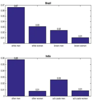
than other groups with similar characteristics. Figure 1.1 shows the share of each group in
highly skilled occupations8in 2010 for Brazil and in 2004 in India. From the figure we see
that white men in Brazil and other men in India are more likely to work in highly skilled
occupations. The most disadvantaged groups in terms of shares in these occupations are
brown men and women in Brazil and other and scheduled caste women in India. All
these groups are less likely than the privileged group to work as executives, architects,
engineers, mathematicians, doctors, and lawyers.
Figure 1.1: Share of groups in highly skilled occupations
Here I show another way of looking at occupational distributions across groups.
I compute an index (Occupational similarity index9) that will show the similarity of
occupational distributions of groups with respect to white men in Brazil and other men
in India. The formula below captures the similarity in occupational distribution across
groups relative to the privileged group:
Ψg= 1−
1 2
N
X
i=1
|pi,wm−pi,g| (1.23)
Ψg is defined as the sum across occupations of the absolute value of the difference
in the propensity of group g relative to white men.10 The index shows the degree of
difference in occupational distribution between groups. An index value of zero implies
that the occupational distribution of the group is not similar to that of white men. A
detailed distribution of the index across groups is presented in Table 1.4. Panels A, B,
9I borrow the index from Hsieh et al. (2013).
and C present the occupational similarity index of the groups relative to the privileged
group in Brazil, India, and the US, respectively. The value of 0.32 for white women in
1991 indicates that the occupational distribution of white women is not similar to that of
white men. The value of 0.82 for brown men in 1991 shows that brown men were closer
to white men in occupational distribution. As can be seen from the table, there is a slight
increase in the index for all groups in Brazil. The index increased from 0.32, 0.82, and
0.28 in 1991 to 0.45, 0.85, and 0.37 in 2010 for white women, brown men and brown
women, respectively.
The occupational distribution analysis for India shows a slightly different picture
than for Brazil. We do not see as high an index value as for brown men in Brazil. The
closest in occupational distribution to other men in India is scheduled caste men with 0.77
in 1993 and 0.81 in 2004. The most disadvantaged in terms of occupational distribution
are other women, with the index of 0.33 in 1993 and 0.37 in 2004. Also the scheduled
caste women did not experience any convergence in occupational distribution relative to
other men, and their index value remained at 0.49.
Panel C of Table 1.4 shows occupational distribution of the groups relative to white
men in the US. We can see that, as in Brazil and India, women in the US have less similar
occupations than men. Women in the US have an occupational distribution closer to
that of white men than do women in other countries. Especially, it is seen in 2010, the
occupational similarity indexes for white and black women are 0.54 and 0.52 versus 0.45
and 0.37 for white and brown women in Brazil, and 0.37 and 0.49 for other and scheduled
caste women in India. Black men in the US are less likely to work in similar occupations
to those of the privileged group than are men in India and Brazil. In 2010 the similarity
index for black men in the US was 0.73, whereas the indexes for brown men in 2010 and
Panel A: Relative to white men in Brazil 1991 2000 2010
white women 0.32 0.36 0.45
brown men 0.82 0.83 0.85
brown women 0.27 0.31 0.37
Panel B: Relative to other men in India 1993 1999 2004
other women 0.33 0.31 0.37
scheduled caste men 0.77 0.76 0.81 scheduled caste women 0.49 0.49 0.49 Panel C: Relative to white men in the US
1990 2000 2010
white women 0.48 0.53 0.54
black men 0.71 0.72 0.73
black women 0.44 0.5 0.52
Table 1.4: Occupational similarity index
1.5.2 Wage gap estimations
As we saw in the previous section, there is a difference in occupational distribution
between groups. Next, I examine if there are differences in wages between groups, their
magnitudes, and if they change over time. From the available data on wages across
occupations, I estimate the wage gaps of the groups relative to white men in Brazil and
to other men in India. The general functional form of log wages can be summarized by
the following equation:
log(wagei) =α+Pgβ1gGig+β2Educi+β3Expi
+β4Exp2i +β5Exp3i+β6Exp4i+
P
kβ7kOik+i
(1.24)
s
where
wage - wage per hour;
Gg - dummy representing groups;
Educi - years of schooling;
Ok - dummy referring to occupations.
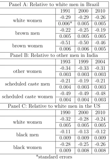
Table 1.5 reports group dummies estimated using the equation 1.24. The value of
-0.29 for white women in Brazil indicates that white women earned 0.29 log points less
than Brazilian white men in 1991. Brown women face the highest disadvantage relative
to white men in terms of wages, with a 0.51 log difference in 1991 and 0.46 in 2010. Wage
gaps for brown men were -0.22, -0.25, and -0.19 in 1991, 2000, and 2010, respectively.
During the 1991–2010 period white and brown women experienced 0.03 and 0.05 log
points wage convergence, respectively.
Panel B reports the estimations of wage gaps relative to other men for groups in
India. Wage gaps relative to other men faced by other women, scheduled caste men, and
scheduled caste women in 1993 were 0.34, 0.21, and 0.49 log points, respectively. There
was no noticeable change in wage gap over time.
Wage gaps of the groups relative to white men in the US show that women earn less
than men with similar characteristics. The wage gaps of the white women and black men
are closer to those of white women and brown men in Brazil. In 2010 white women and
black men earned 0.24 and 0.12 log points lower than white men, whereas white women
and brown men earned 0.26 and 0.19 log points lower than white men in Brazil. The
earnings of black women in the US are closer to those of white men than the earnings of
Panel A: Relative to white men in Brazil
1991 2000 2010
white women -0.29 -0.29 -0.26
0.006* 0.005 0.005
brown men -0.22 -0.25 -0.19
0.005 0.005 0.005
brown women -0.51 -0.50 -0.46
0.006 0.006 0.005 Panel B: Relative to other men in India
1993 1999 2004
other women -0.34 -0.33 -0.31
0.003 0.003 0.003
scheduled caste men -0.21 -0.19 -0.21 0.004 0.003 0.003
scheduled caste women -0.49 -0.49 -0.48 0.004 0.004 0.003 Panel C: Relative to white men in the US
1990 2000 2010
white women -0.32 -0.28 -0.24
0.005 0.005 0.005
black men -0.11 -0.13 -0.12
0.009 0.009 0.009
black women -0.28 -0.25 -0.26
0.009 0.008 0.008 *standard errors
Table 1.5: Conditional log difference in wages
The model predicts that wage gaps are the same for all occupations (1.16) and
independent of propensities. This means that changes in frictions faced by a group in
one occupation, resulting in a change of relative propensities, does not affect the average
wage of the group, because an increase (a decrease) of a friction will attract (deter) less
qualified workers, thus lowering (increasing) the average quality of the group. Table 1.6
shows the results of the regression of the occupational wage gap and relative propensities.
The regression was weighted by the share of the workers in the groups across occupations.
As can be seen from the table, the slope and the R2 from the regression of the wage
gap on propensities are small for all three countries, which is an indication that there is
equation.
1991 2000 2010
slope st_dev R2 slope st_dev R2 slope st_dev R2
white women -0.021 0.020 0.016 -0.023 0.020 0.019 0.021 0.015 0.031 brown men 0.009 0.026 0.002 0.026 0.031 0.010 0.015 0.022 0.007 brown women -0.041 0.022 0.052 0.010 0.021 0.004 -0.003 0.019 0.000
(a) Brazil
1993 1999 2004
slope st_dev R2 slope st_dev R2 slope st_dev R2
other women -0.014 0.025 0.005 -0.035 0.018 0.059 -0.018 0.021 0.011 sc.caste men 0.059 0.036 0.040 0.008 0.034 0.001 -0.026 0.034 0.009 sc.caste women -0.014 0.028 0.004 -0.016 0.023 0.008 -0.030 0.026 0.019
(b) India
1990 2000 2010
slope st_dev R2 slope st_dev R2 slope st_dev R2
white women 0.005 0.024 0.001 -0.008 0.020 0.003 0.006 0.020 0.001 black men 0.032 0.034 0.065 0.036 0.026 0.066 0.007 0.021 0.002 black women 0.020 0.026 0.009 0.021 0.021 0.015 0.001 0.027 0.000
(c) USA
Table 1.6: Relationship of wage gaps and propensities
1.5.3 Estimation of Frictions
From the available data on the fraction of people in groupg who work in occupation
i (pig) and the wage of group g relative to privileged group ( ¯wg/w¯g0), I can estimate the
relative frictions faced by groups in Brazil and India. So, by rearranging equation (1.17),
I arrive at the following estimate of the composite friction ˆτig for each group in each
occupation:
ˆ
τig=
τig
τiwm
(Tiwm
Tig
)1θ = ( pig
piwm
)−1θ( w¯g ¯
wwm
)−(1−η) (1.25)
ˆ
τig is called a composite friction because it is a function of both relative friction
τig
τiwm and relative mean talent (
Tiwm
the relative propensity of the group pig
piwm is low (the group is underrepresented in this
occupation) or the group faces a low wage gap w¯g ¯
wwm. The right-hand side of the equation
is observed in the data, so we can use it to determine ˆτig faced by each group in each
occupation. The calculation of the friction by using the formula requires the estimates
of θ (the parameter that governs the dispersion of talent) and η (the elasticity of human
capital with respect to expenditure on human capital). I use the baseline parameter
estimates from Hsieh et al. (2013) and conduct robustness checks later. The baseline
parameter values are given in Table 1.7. With the baseline parameter value for θ equal
to 3.44, and baseline parameter value for η equal to 0.25, I compute composite frictions.
Parameter Value
Elasticity of substitution σ 3
Skill dispersion parameter θ 3.44
Elasticity of human capital η 0.25
Parameter in the utility β 0.693
Table 1.7: Baseline parameter values
Table 1.8 shows the estimates of the mean and standard deviation of ˆτig faced by
the groups in all periods for Brazil, India, and the US. A value of the friction equal to
one means a group faces no frictions relative to a privileged group. If the value is more
than 1 then a group faces a friction, while a value less than 1 acts like a subsidy for that
group in that occupation.
In Brazil the highest frictions are faced by brown women, the average friction for
this group is 2.41 in 1991. The variance of frictions for the group is also the highest:
in 1991 the standard deviation was 1.13. Over twenty years, the friction experienced by
brown women in Brazil decreased: in 2010 the mean and standard deviation are 1.99 and
0.70, respectively. Of the three groups in Brazil, brown men face the least frictions. In
1991 the average friction for this group was 1.31, which only decreased by 0.10 to 1.20
in twenty years. The standard deviation of the frictions considerably decreased over the
shows that frictions for these groups are highly dispersed across occupations. As shown
by equation 1.17, dispersion of frictions across occupations causes misallocation of the
talent.
For India we see that the frictions are the highest for scheduled caste women and
other women. The average frictions are 2.24 and 2.79 in 1993, respectively for other and
scheduled caste women. In 2004 these decreased slightly to 2.09 and 2.64, respectively.
Scheduled caste women also face the higher dispersion of frictions than do other women.
The dispersion is 1.26 for scheduled caste women versus 0.80 for other women in 1993, and
these did not change much over the period. The lowest friction is faced by scheduled caste
men: the average friction for the group is 1.34 and 1.26, in 1993 and 2004, respectively.
The magnitude of frictions faced by the scheduled caste men in India is comparable to
the that of brown men in Brazil.
The frictions faced by the groups in the US are lower than those of the groups in
India and Brazil. The frictions faced by women are higher than the frictions faced by black
men. Black women face slightly higher frictions than do white women. The dispersion
of frictions for black women is also higher than that of white women. Overall, the table
1991 2000 2010
mean st_dev mean st_dev mean st_dev
white women 1.77 0.64 1.86 0.93 1.57 0.52
brown men 1.31 0.25 1.32 0.23 1.20 0.14
brown women 2.41 1.13 2.42 1.13 1.99 0.70
(a) Brazil
1993 1999 2004
mean st_dev mean st_dev mean st_dev
other women 2.24 0.80 2.29 1.10 2.09 0.73
sc. caste men 1.34 0.21 1.29 0.18 1.26 0.15
sc. caste women 2.79 1.26 2.54 0.95 2.64 1.33
(b) India
1990 2000 2010
mean st_dev mean st_dev mean st_dev
white women 1.55 0.58 1.46 0.52 1.45 0.53
black men 1.11 0.18 1.15 0.21 1.18 0.29
black women 1.62 0.85 1.53 0.76 1.59 0.73
(c) USA
Table 1.8: Summary stats of frictions across countries
1.6 Results
There are 8 exogenous parameters: Ai (technology by occupation), φi (elasticity of
human capital with respect to schooling),τig(frictions by occupation and group),qg(total
number of people by group),θ(the parameter that governs the dispersion of talent),η(the
elasticity of human capital with respect to expenditure on human capital), σ (elasticity
of substitution between occupations), and β (weight on consumption relative to time in
the utility function). The baseline values of some parameters are given in Table 1.7. I
check for robustness with different parameter values.
The number of people in each group qg is taken from the data. Assuming that
τigh captures the efficiency in human capital accumulation, I set ¯hig to one. I normalize
mean talent across groups for each occupation as Tig = 1. The normalization Tig = 1
the same across occupations within groups. From the equation on average wage gaps and
equilibrium condition for schooling and matching the wage gap in the data I estimateφi
for each occupation. The technology parameter across occupations Ai is estimated from
equations 1.22, 1.20, and 1.21. Values for the price of efficiency units of human capital
wi are obtained by using equation 1.13 and matching to the data.
1.6.1 Model fit
Given these parameters I can compare the results produced by the model with
the data. In particular, I compare the model and data version of mean earnings and
occupational shares across groups and occupations. In the model, equation 1.13 produces
the occupational shares across groups and occupations and equation 1.15 produces mean
earnings across groups and occupations.
The model is calibrated to the occupational shares of white men in each period.
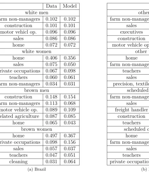
Table 1.9 compares the occupational shares produced by the model with the data for
the five occupational categories with the highest shares for each group. For example,
according to the data, the share of white men in Brazil working as farm non-managers is
0.102. The model counterpart of the data is also 0.102. For other groups in Brazil the
model produces close results. According to the data, 40.6% of white women and 49.7%
of brown women work in home sector. The model shows that 35.6% of white and 36.7%
of brown women work in home sector.
In India most men work as farm non-managers and most women work in the home
sector. The data shows that in 2004 33% of other men and 42% of scheduled caste
men were occupied in farming. The model versions of these shares are 33% and 40%,
respectively for other and scheduled caste men. In the same period 63.4% of other women
and 48.6% of scheduled caste women were occupied in home sector. The model predicts
Data Model white men
farm non-managers 0.102 0.102 construction 0.101 0.101 motor vehicl op. 0.096 0.096
sales 0.086 0.086
home 0.072 0.072
white women
home 0.406 0.356
sales 0.075 0.050
private occupations 0.067 0.098
teachers 0.060 0.061
farm non-managers 0.034 0.031 brown men
construction 0.148 0.154 farm non-managers 0.113 0.068 motor vehicle op. 0.089 0.109 related agriculture 0.087 0.085
home 0.065 0.043
brown women
home 0.497 0.367
private occupations 0.098 0.156
sales 0.057 0.037
teachers 0.047 0.051
cleaning 0.031 0.064
(a) Brazil
Data Model
other men
farm non-managers 0.330 0.330
sales 0.148 0.148
executives 0.050 0.050
construction 0.044 0.044 motor vehicle op. 0.040 0.040
other women
home 0.634 0.615
farm non-managers 0.219 0.225
teachers 0.022 0.022
sales 0.021 0.024
precision, textile 0.019 0.016 scheduled caste men
farm non-managers 0.422 0.400
sales 0.071 0.066
freight handler 0.067 0.062 construction 0.067 0.056
teachers 0.046 0.060
scheduled caste women
home 0.486 0.460
farm non-managers 0.354 0.351
sales 0.025 0.024
teachers 0.018 0.025
private occupations 0.016 0.004
(b) India
Table 1.9: Occupational shares in Brazil and India (data vs model)
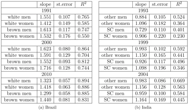
Table 1.10 shows the results of regressing the earnings data on the model version of
earnings for each group and period in Brazil and India. For Brazilian white men in 1991,
a value of 1.551 indicates that a 1 percent increase in mean earnings of white men in 1991
produced by the model corresponds to a 1.551 percent increase in mean earnings given
by the data. Overall, the model produces less earnings than data. As can be seen from
the table in Brazil the model produces the highest fit for white men in 2010 with an R2
of 0.894. The lowest fit corresponds to the earnings of brown women in 1991 with an R2
of 0.550.
of the slope than for Brazil. Overall, 1 percent increase in mean earnings produced by
the model corresponds to 0.8–1.15 percent increase in mean earnings given by the data.
However, the percentage of the variation in the the data that the model explains is lower
in India than in Brazil. The lowest fit belongs to scheduled caste women in 1991 with an
R2 of 0.230 and other men in 2004 anR2 of 0.669.
slope st.error R2
1991
white men 1.551 0.107 0.765
white women 1.412 0.149 0.585
brown men 1.613 0.117 0.747
brown women 1.532 0.176 0.550 2000
white men 1.623 0.080 0.864
white women 1.591 0.129 0.704
brown men 1.552 0.093 0.812
brown women 1.716 0.128 0.744 2010
white men 1.323 0.057 0.894
white women 1.418 0.063 0.886
brown men 1.299 0.058 0.885
brown women 1.440 0.081 0.831
(a) Brazil
slope st.error R2
1993
other men 0.884 0.105 0.524
other women 1.096 0.182 0.364
SC men 0.729 0.110 0.401
SC women 0.906 0.220 0.230
1999
other men 0.993 0.102 0.592
other women 1.150 0.165 0.441
SC men 0.926 0.117 0.496
SC women 1.098 0.196 0.346
2004
other men 0.983 0.086 0.669
other women 1.156 0.128 0.563
SC men 0.959 0.100 0.584
SC women 1.164 0.169 0.445
(b) India
Table 1.10: Mean earnings across groups in Brazil and India (data vs model)
1.6.2 Output gain
Since I have all the exogenous parameters, I can compute aggregate output from
the model. Then I can investigate how changing frictions affects the output. Since I have
data only for aggregate frictions τig =
(1+τigh)η 1−τw
ig , I can not separately identify the effects
from τigw and τigh. So, I do the analysis for two different cases: a case in which I allow
frictions only in acquisition of human capitalτigh, and a case in which only frictions in the
labor marketτigw are allowed.
I explore several counterfactuals. In a baseline case, I compute aggregate output in
eliminating all frictions, and using US frictions. Earlier I showed frictions faced by the
groups in US. In this section I check if replacing frictions faced by the groups in Brazil
and India with those of the US affects the aggregate productivity in these countries. In a
robustness check section, I test the counterfactual output gain due to zero frictions with
different parameter values.
Counterfactual output gain in Brazil
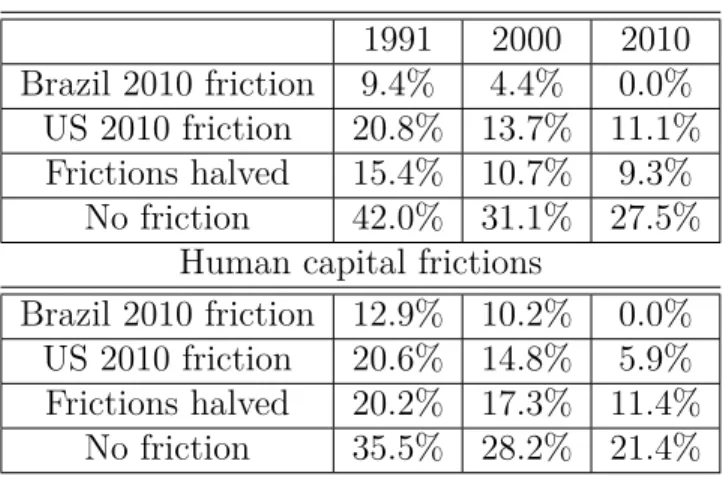
Table 1.11 presents output gain in Brazil with various frictions. The top panel of
the table shows output gain due to frictions in the labor market and the bottom panel
shows output gain due to frictions in accumulation of human capital. The output gain is
higher if frictions were replaced by the 2010 frictions in Brazil as shown in the first row of
the table. In the case of frictions in the labor market if the 1991 and 2000 frictions were
replaced by the 2010 frictions, the output would increase by 9.4% and 4.4%, respectively.
The second row shows the gain with the US frictions in 2010. The gains are 20.8%, 13.7%
and 11.1%. From the previous sections, I showed that the 2010 frictions in Brazil are
lower than in other periods, and that the frictions in the US are also lower than those
in Brazil in corresponding periods. Thus, the analysis shows that output increases with
the reduction of frictions. The last two rows show the counterfactual output gain from
halving the frictions in corresponding years and removing them. Halving the frictions
faced by the groups across occupations increases the output by 15.4%, 10.7%, and 9.3%.
Removing them entirely increases the output even more by 42%, 31.1%, and 27.5%.11
Output gain due to acquisition of human capital shows a similar pattern in output gain,
but the gain is lower than with frictions due to the labor market.The gain increases both
with τigw and τigh cases. In the τigh case eliminating frictions has a smaller effect compared
to theτigw case.
Frictions in labour market
1991 2000 2010
Brazil 2010 friction 9.4% 4.4% 0.0% US 2010 friction 20.8% 13.7% 11.1% Frictions halved 15.4% 10.7% 9.3%
No friction 42.0% 31.1% 27.5%
Human capital frictions
Brazil 2010 friction 12.9% 10.2% 0.0% US 2010 friction 20.6% 14.8% 5.9% Frictions halved 20.2% 17.3% 11.4%
No friction 35.5% 28.2% 21.4%
Table 1.11: Counterfactuals: Output gain in Brazil
Counterfactual output gain in India
For India I first show the results of the model with the limited number of caste
categories but detailed occupational categories. Then I investigate if results change with
more detailed caste categories but broader occupational categories. I do this because the
data size is small with detailed caste and detailed occupation categories. So there is a
trade-off between the number of caste categories and the number of occupation categories.
Broader caste categories. Table 1.12 presents counterfactuals output gain in India
due to labor market frictions (τigw) on the top and frictions in human capital (τigh) on
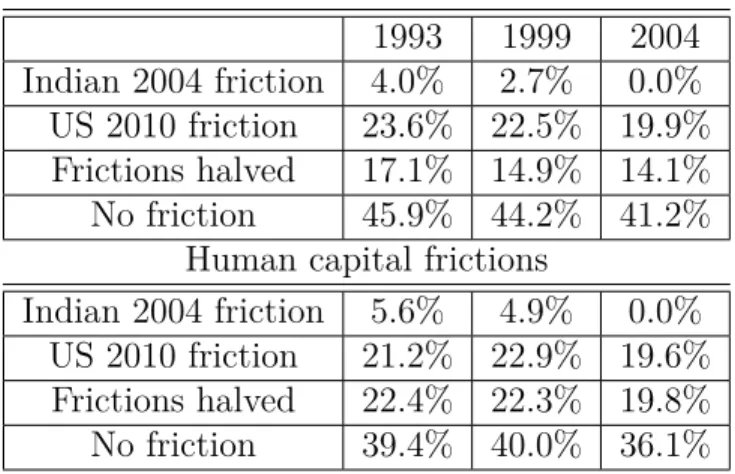
the bottom panel. The following four cases are investigated: output gain if frictions
were replaced by 2004 Indian frictions, gain with US 2010 frictions, gain if frictions were
halved, and gain if frictions were removed. Replacing the 1993 and 1999 frictions in India
with 2004 frictions increases production in 1993 and 1999 by 4% and 2.7%, respectively,
meaning that frictions in 2004 were slightly less than in 1993 and 1999. If frictions faced
by the groups were replaced by those of the groups in the US in 2010 the output would
increase by 23.6%, 22.5%, and 19.9%, respectively in 1993, 1999, and 2004. Cutting
frictions to half in all groups across all occupations increases the output even more, by
17.1%, 14.9%, and 14.1% in the corresponding years. We observe higher gains than in
output by 45.9% in 1993 and by 44.2% and 41.2% in 1999 and 2004. The model predicts
that output increases with reducing frictions. The gain increases both with τigh and τigw
cases. In the τigh case eliminating frictions has a smaller effect compared to the τigw case.
Frictions in labour market
1993 1999 2004
Indian 2004 friction 4.0% 2.7% 0.0% US 2010 friction 23.6% 22.5% 19.9% Frictions halved 17.1% 14.9% 14.1%
No friction 45.9% 44.2% 41.2%
Human capital frictions
Indian 2004 friction 5.6% 4.9% 0.0% US 2010 friction 21.2% 22.9% 19.6% Frictions halved 22.4% 22.3% 19.8%
No friction 39.4% 40.0% 36.1%
Table 1.12: Counterfactuals: Output gain in India
Detailed caste categories. Here I show the results generated by using detailed caste
categories. The categories available for all periods are “other”, “scheduled tribe”, and
“scheduled caste”. I use only 19 broad occupation categories as opposed to the 67
occupa-tion codes used in the previous analysis. The broader categories are aggregated by using
67 occupations. These 19 occupation categories are shown in Appendix Table A2.
Table 1.12 shows the effect of reducing frictions faced by different groups on
aggre-gate production in India. The column headings refer to the number of caste categories.
The column 2 shows the output gain with 3 caste categories and column 3 shows the
output gain with 2 caste categories. As can been seen from the table the output gain
is close in both cases. The counterfactual output gain from removing all frictions with
detailed castes increases the aggregate output by 34%, 31.1%, and 28.7% in 1993, 1999,
and 2004, respectively. The counterfactual output gain from removing all frictions with
broad castes increases the aggregate output by 33.6%, 30.9%, and 28% in 1993, 1999, and
2004, respectively.
detailed caste categories removing frictions in all occupations faced by the groups results
in increase of the output by 33.9%, 31.7%, and 28.9% in 1993, 1999, and 2004, respectively.
The counterfactual gain in the case of broad caste categories is also significant: the output
goes up by 33.1%, 31.1%, and 27.9% in the respective years.
more castes less castes due to labor market
1993 34.0% 33.6%
1999 31.1% 30.9%
2004 28.7% 28.0%
due to human capital
1993 33.9% 33.1%
1999 31.7% 31.1%
2004 28.9% 27.9%
Table 1.13: Counterfactuals: Output gain in India with detailed caste categories
Gains in Brazil vs. India
The output gains from reducing frictions are larger in India than in Brazil. According
to the model, there are three forces that vary across countries and that affect output gains
from removing frictions: occupational shares, wage gaps, and population shares. Here I
investigate which of these three forces is most important for larger gains in India than
in Brazil. To do that I compute output in India by replacing each of the three items
in India with that of Brazil. Then I compare counterfactual output gains in India by
removing frictions. Table 1.14 shows the results in the case of frictions in labor market
and friction in human capital, respectively. The first row shows the baseline case with
occupational shares, wage gaps and population shares in India where the gain in output
is due to removing frictions.
The second row of Table 1.14 illustrates how changes in wage gaps in India affect
the output of the country. This is a counterfactual in which wage gaps of the groups in
India are replaced by the wage gaps of the groups in Brazil. The effects of changing the
in all years. This indicates that wage gaps faced by the groups in Brazil and India are
similar in corresponding years.
The third row of the table shows the counterfactual gain if the Indian population
shares were replaced by Brazilian population shares. That is, the population shares of the
four groups in each period in India are replaced with the population shares of the four
groups in Brazil in corresponding periods, holding everything else fixed. This will produce
the output gain from removing frictions in the case of frictions in labor market of 53.5%,
52.7%, and 52.2%, and in case of frictions in human capital of 44%, 45.8%, and 43% in
1993, 1999, and 2004, respectively. The gain is larger with Brazilian population shares
than with Indian population shares. This is not surprising since the share of disadvantaged
groups in India is smaller than the share of disadvantaged groups in Brazil, and reducing
frictions for groups with larger population share will have a larger effect on output.
The last row shows the productivity effects of replacing the occupational shares in
India with the occupational shares in Brazil, holding everything else fixed. Removing
frictions will result in 34.7%, 31.1%, and 28.6% increase in output in the case of the
frictions in labor market and in 27%, 25.7%, and 15.8% increase in output in the case
of the frictions in human capital, in corresponding years. The gains are smaller with
Brazilian occupational shares than with Indian occupational shares. This shows that in
1993 1999 2004
Baseline 45.9% 44.2% 41.2%
with Brazilian wage gaps 45.9% 44.6% 41.7% with Brazilian population shares 53.5% 52.7% 52.2% with Brazilian occupational shares 34.7% 31.1% 28.6%
(a) Frictions in the labor market
1993 1999 2004
Baseline 39.4% 40.0% 36.1%
with Brazilian wage gaps 39.4% 40.1% 36.3% with Brazilian population shares 44.0% 45.8% 43.0% with Brazilian occupational shares 27.0% 25.7% 15.8%
(b) Frictions due to human capital
Table 1.14: Counterfactual output growth in India
1.6.3 Robustness analysis
In this section, I test the previous results for robustness. I compute the output gain
with different values of θ, η, and σ. The exercise is done separately by allowing frictions
in the labor market and in the acquisition of human capital. The results in Table 1.15
and Table 1.16 show the gain in output in 2010 for Brazil and in 2004 for India when all
frictions are removed.
The first row of Table 1.15 shows the output gain in Brazil due to removing frictions
with changing η, holding other parameters constant. As can be seen, the results with
changing η are robust. The gain does not change much with changing σ, except for
σ= 15. The change in gain from the baseline case when σ= 15 is 4–6%. With changing
Frictions due to labor market
η= 0.25 η= 0.15 η= 0.5 η= 0.1
changingη 27.5% 27.5% 27.5% 27.5%
σ= 3 σ= 4.5 σ= 15 σ= 2.75
changing σ 27.5% 29.8% 32.8% 26.9%
θ= 3.44 θ= 4.16 θ= 5.6 θ= 8.4
changing θ 27.5% 27.5% 27.5% 27.5%
Frictions due to human capital
η= 0.25 η= 0.15 η= 0.5 η= 0.1
changingη 21.4% 19.3% 27.4% 18.3%
σ= 3 σ= 4.5 σ= 15 σ= 2.75
changing σ 21.4% 23.0% 25.1% 20.9%
θ= 3.44 θ= 4.16 θ= 5.6 θ= 8.4
changing θ 21.4% 20.1% 18.4% 16.4%
Table 1.15: Output gain in Brazil due to removed frictions
The results in Table 1.16 display the gain in output in 2004 with changing parameters
in India. For the case with friction in the labor market, changingη does not change the
gain in output relative to the baseline case. With changingσ, the output varies from the
baseline by 20% whenσ= 15. Varying θ shows no difference from the baseline gain.
The pattern of output gain in the case of frictions in human capital acquisition is
different from frictions in the labor market. The gain differs from the baseline by 4–5%