Brown_unc_0153D_15479.pdf

(1)

CASE STUDIES ON OPTIMIZING ALGORITHMS

FOR GPU ARCHITECTURES

Shawn Daniel Brown

A dissertation submitted to the faculty of the University of North Carolina at Chapel Hill in partial fulfillment of the requirements for the degree of Doctor of Philosophy in the Department

of Computer Science in the College of Arts & Sciences.

Chapel Hill 2015

(2)

(3)

iii

ABSTRACT

SHAWN DANIEL BROWN: Case Studies on Optimizing Algorithms for GPU Architectures (Under the direction of Jack Snoeyink)

Modern GPUs are complex, massively multi-threaded, and high-performance.

Programmers naturally gravitate towards taking advantage of this high performance for achieving faster results. However, in order to do so successfully, programmers must first understand and then master a new set of skills – writing parallel code, using different types of parallelism, adapting to GPU architectural features, and understanding issues that limit performance.

To help GPU programmers become productive more quickly, this dissertation introduces three data access skeletons (DASks) – Block, Column, and Row -- and two block access

skeletons (BASks) – Block-By-Block and Warp-by-Warp. Each “skeleton” provides a high-performance implementation framework that partitions data arrays into data blocks and then iterates over those blocks. Programmers must still write “body” methods on individual data blocks to solve their specific problem. These skeletons provide efficient machine dependent data access patterns for use on GPUs. DASks group n data elements into m fixed size data blocks. These m data block are then partitioned across p thread blocks using a 1D or 2D layout pattern. Generic programming techniques are applied to the fixed size data blocks to enable performance experiments for different types of parallelism – instruction-level parallelism (ILP), data-level parallelism (DLP), and thread-level parallelism (TLP).

These different DASks and BASks are introduced using a simple memory I/O (Copy) case study. Three additional case studies – Reduce/Scan, Histogram, and Radix Sort --

(4)

iv

To Helene, my love, my rock, my soul mate your love has helped support and guide me through these many tough years working on my PhD. You showed great wisdom, love, and courage during some turbulent times within our family.

Proverbs 31:10-31

(5)

v

ACKNOWLEDGMENTS

(6)

vi

LIST OF TABLES

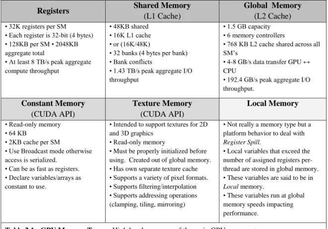
Table 2.1 GPU Memory Types ... 28

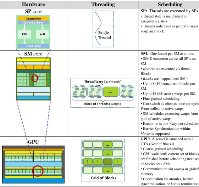
Table 2.2 GPU Threading and Scheduling Model ... 33

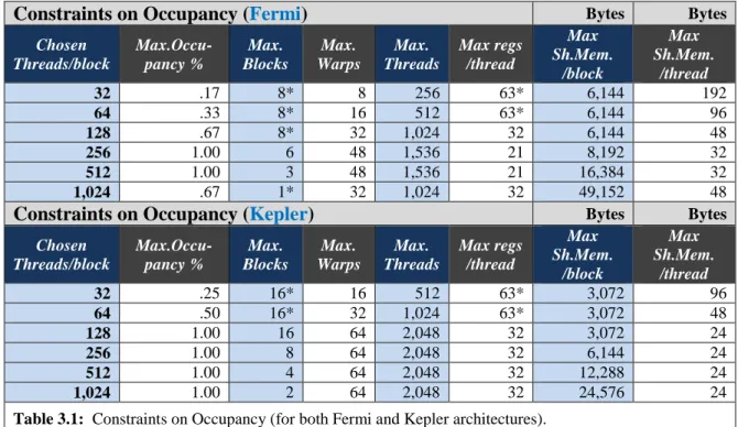
Table 3.1 Constraints on Occupancy (Fermi and Kepler) ... 55

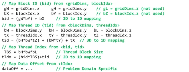
Table 4.1 Mapping CTA parameters (Code Snippets) ... 71

Table 5.1 Loop Unrolling vs. Software Pipelining Performance ... 103

Table 5.2 Modifications to the Block DASk to support Fill, Copy, Scatter, and Gather... 109

Table 5.3 Load balancing data blocks for the ‹FIRST?›‹MIDDLE*›‹LAST?› Pattern ... 123

Table 5.4 Batching vs. Interleaving Memory Accesses ... 127

Table 6.1 Common Associative Operators ... 132

Table 6.2 Reduce Scan Nomenclature and Symbols ... 133

Table 6.3 Serial Reduce and Inclusive/Exclusive Serial Scan ... 134

Table 6.4 Best Reduce / Scan Throughput Results ... 135

Table 6.5 Adder Summary ... 139

Table 6.6 GPU_Reduce / GPU_Scan Template Parameters ... 170

Table 6.7 GPU_Reduce / GPU_Scan Function Parameters ... 171

Table 6.8 GPU_Reduce / GPU_Scan CTA Parameters ... 171

Table 6.9 Convert between Warp and Sequential data views ... 173

Table 6.10 Padding for a given run length to avoid Bank Conflicts ... 175

Table 6.11 Reduce/Scan Experiment Environment ... 179

Table 6.12 Best Case Reduce/Scan Results... 180

Table 6.13 TLP Reduce/Scan Results ... 180

Table 6.14 ILP Reduce/Scan Results ... 181

Table 6.15 Best ‹TLP,ILP› Summary ... 182

(15)

xv

Table 6.17 Total Cycle Results ... 184

Table 7.1 Nearest Neighbor Search Types ... 192

Table 7.2 NN Search Experiment Environment ... 210

Table 7.3 CPU Build Performance ... 211

Table 8.1 Histogram Test Environment ... 234

Table 8.2 CUDA Profiler Results ... 239

Table 9.1 GPU_CountKeys C++ Template Parameters ... 259

Table 9.2 GPU_CountKeys Function Parameters... 260

Table 9.3 GPU_CountKeys CTA Parameters ... 260

Table 9.4 GPU_DistributeKeys C++ Template Parameters... 271

Table 9.5 GPU_DistributeKeys Function Parameters ... 272

Table 9.6 GPU_DistributeKeys CTA Parameters ... 273

Table 9.7 Bank Conflicts for Increasing run length ... 282

Table 9.8 Coalesced I/O Efficiency (for increasing DBS) ... 301

Table 9.9 Radix Sort Experiment Environment ... 304

Table 9.10 Maximum Data Throughput (on GTX 580) ... 305

Table 9.11 Maximum Data Throughput (on GTX Titan) ... 306

Table 9.12 Total Cycles (GPU_CountKeys Kernel) ... 308

(16)

xvi

LIST OF FIGURES

Figure 2.1 Flynn’s Taxonomy ... 15

Figure 2.2 Serial vs. Parallel Machine Models ... 16

Figure 2.3 Memory Hierarchy ... 20

Figure 2.4 CPU vs. GPU core in Broad Themes ... 22

Figure 2.5 Modern GPU core layout ... 25

Figure 3.1 Histogram I/O throughput ... 43

Figure 3.2 Work and Depth Example ... 45

Figure 3.3 Simple CTA mapping ... 50

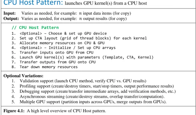
Figure 4.1 CPU Host Pattern Overview ... 64

Figure 4.2 CPU Host Pattern Example ... 65

Figure 4.3 Computing a CTA layout ... 68

Figure 4.4 Serial, Parallel, and GPU Copy programs ... 76

Figure 4.5 Simple Copy Throughput for Increasing n ... 80

Figure 5.1 Copy Performance ... 84

Figure 5.2 The Block Data Access Skeleton (DASk) ... 85

Figure 5.3 Block Access Skeletons (Block-by-Block vs. Warp-by-Warp) ... 87

Figure 5.4 Amortized Range Checking (Block DASk) ... 90

Figure 5.5 Amortized Pointer Indexing ... 93

Figure 5.6 Block DASk Code ... 94-95 Figure 5.7 Automatic Loop Unrolling Example ... 98

Figure 5.8 Automatic Loop Unrolling vs. Manual Loop Unrolling Throughput ... 99

Figure 5.9 Manual Loop Unrolling Example ... 101

Figure 5.10 Copy Throughput for Increasing block size ... 106

Figure 5.11 Copy Throughput for an Increasing number of concurrent blocks per SM ... 107

(17)

xvii

Figure 5.13 Column DASk Code... 114-115

Figure 5.14 The Row DASk ... 118

Figure 5.15 Warp Aligning Data Access ... 119

Figure 5.16 Row DASk Code with the ‹FIRST?›‹MIDDLE*›‹LAST?› Pattern ... 121-122 Figure 5.17 Load Balancing Code for the Row DASk ... 124-125 Figure 6.1 Full Reduce/Scan Throughput Results ... 136

Figure 6.2 Hardware Adder Diagrams ... 140

Figure 6.3 Parallel Reduce Patterns (Tree-Reduce and Run-Reduce) ... 142

Figure 6.4 Parallel Scan Patterns (Scan-then-Fan and Reduce-then-Scan) ... 143

Figure 6.5 GPU Reduce and Scan (High Level Overview) ... 148

Figure 6.6 RunLoad Method (Code) ... 150

Figure 6.7 SerialReduce and SerialScan Methods (Code) ... 152

Figure 6.8 SerialScan Total Cycles (Comparison) ... 153

Figure 6.9 Overloaded Add Functors (CPU and GPU) ... 154

Figure 6.10 WarpScan Layout Diagram ... 155

Figure 6.11 WarpScan Total Cycles (Comparison) ... 156

Figure 6.12 WarpReduce and WarpScan Methods (Code) ... 157

Figure 6.13 RunUpdate Method (Code) ... 158

Figure 6.14 BlockReduce Method (Code) ... 161

Figure 6.15 BlockScan Method (Code) plus Setup Hints ... 162-163 Figure 6.16 GPU_Scan Kernel (High level Code Overview) ... 168-169 Figure 6.17 Pad and Rake Technique (Overview) ... 176

Figure 6.18 Bank Conflict Comparison ... 183

Figure 7.1 Brute Force Spatial Search ... 194

(18)

xviii

Figure 7.3 A kd-tree ... 195

Figure 7.4 A kd-tree Trim Test ... 197

Figure 7.5 kd-tree Search ... 198

Figure 7.6 kd-tree Build and Search Methods (Code) ... 205

Figure 7.7 kd-tree Search Results ... 212

Figure 8.1 256-bin CPU Histogram Method (Code) ... 218

Figure 8.2 Bit-Level Parallelism ... 219

Figure 8.3 TRISH Layout ... 223

Figure 8.4 Staggered Start / Circular Indexing (Code Snippets) ... 225

Figure 8.5 BLP Optimization ... 227

Figure 8.6 Binning Code ... 228

Figure 8.7 Row-Sum Efficiency ... 230

Figure 8.8 GPU_Count Kernel ... 232

Figure 8.9 Synthetic Data Throughput ... 235

Figure 8.10 Image Data Throughput ... 237

Figure 9.1 Serial Counting Sort (Code) ... 252

Figure 9.2 Serial LSD Radix Sort (Code) ... 253

Figure 9.3 GPU Counting Sort (3 Kernel Diagram) ... 256

Figure 9.4 GPU_CountKeys Kernel (Code Overview) ... 258

Figure 9.5 Sequential vs. Pipelined Counting Performance Bottleneck (Code Snippets) ... 262

Figure 9.6 Handling Potential Overflow (Code Snippet) ... 263

Figure 9.7 GPU_ScanRuns Kernel (Code Overview) ... 266

Figure 9.8 GPU_DistributeKeys Kernel (Code Overview) ... 269-270 Figure 9.9 Loading Keys Efficiently ... 281

Figure 9.10 Extract Digits from Keys ... 284

(19)

xix

Figure 9.12 ScanWarps Method Overview ... 287

Figure 9.13 ScanWarps Method (Code) ... 289

Figure 9.14 Handle Overflow by Upscaling ... 291

Figure 9.15 ScanBlocks Memory Layout ... 293

Figure 9.16 ScanBlocks Overview ... 294

Figure 9.17 Local Start = warp-start + thread-start + key-start ... 296

Figure 9.18 ShuffleKeys (Sorting Increases Coherence) ... 300

Figure 9.19 Full Radix Sort Data Throughput Results ... 307-308 Figure 10.1 BASks Review (Block-by-Block and Warp-by-Warp) ... 325

Figure 10.2 The Block DASK Review ... 327

Figure 10.3 The Column DASK Review ... 328

(20)

xx

LIST OF ABBREVIATIONS

ALU Arithmetic Logic Unit

All-𝑘NN All 𝒌 Nearest Neighbor (search) All-NN All Nearest Neighbor (Search)

AMP Accelerated Massive Parallelism (Microsoft) ANN Approximate Nearest Neighbor (Search) API Application Program Interface

b, B Bit or boolean {0|1} or {true|false} BASk Block Access Skeleton

BFS Breath First Search

bid block id (uniquely identifies thread block within grid) BLP Bit-Level Parallelism

BPS Bits Per Second

BSP Binary Space Partition (tree)

BYTE Derived from ‘bit’ and ‘bite’ (8-bits of data) CC Clock Cycle or Compute Capability

CPI (average) Cycles Per Instruction (for entire algorithm) CPU Central Processing Unit

CTA Cooperative Thread Array (Grid of Thread Blocks) CUDA Compute Unified Device Architecture (NVIDIA) DASk Data Access Skeleton

DBS Data Block Size

DDR Double Data Rate memory type (as in DDR3-RAM) DFS Depth First Search

(21)

xxi DWORD Double Word (32-bits of data, 4 bytes) EX Execute cycle (classic MIPS pipeline) FMA Fused Multiply Add instruction (in ISA) FPU Floating Point Unit

G Giga (one billion)

GB Giga-Byte (one billion bytes) GM Global Memory

GPU Graphics Processing Unit HPC High Performance Computing

ID Instruction Decode cycle (classic MIPS pipeline) IDE Interactive Development Environment

IF Instruction Fetch cycle (classic MIPS pipeline) II (total) Instructions Issued (for entire algorithm) ILP Instruction-Level Parallelism

IPC (average) Instructions (retired) Per Cycle ISA Instruction Set Architecture

K Kilo (one thousand)

KB Kilo-Byte (one thousand bytes) kd k-Dimensional

kd-tree A generalized binary tree used for spatial searching

𝑘NN 𝒌 Nearest Neighbor (search)

KSHS Kogge-Stone-Hillis-Steele prefix-sum (scan) LSD Least Significant Digit

M Mega (one million)

MB Mega-Byte (one million bytes)

(22)

xxii MISD Multiple-Instruction, Single Data MIMD Multiple-Instruction, Multiple Data

MIPS Microprocessor (without) Interlocked Pipeline Stages MPI Message Passing Interface

MPMD Multiple-Program, Multiple-Data MSD Most Significant Digit

NN Nearest Neighbor (Search) NOP No Operation

octree A 3D hierarchical spatial searching data structure OpenCL Open Computing Language (Khronos Group) PTX Parallel Thread Execution assembly code (NVIDIA) quadtree A 2D hierarchical spatial searching data structure QNN Query Nearest Neighbor (search)

QWORD Quad Word (64-bits of data, 8 bytes)

RB Reach Back (convert inclusive to exclusive scan) RAM Random-Access Memory

RAW Read After Write (data hazard) RISC Reduced Instruction Set Computer RNN Range (Nearest Neighbor) Query Search RAM Random Access Memory

SM Shared Memory Sh. Mem. Shared Memory

SIMD Single-Instruction, Multiple-Data SIMT Single-Instruction, Multi-Threaded SISD Single-Instruction, Single-Data

(23)

xxiii

SMX Streaming Multi-core Extended (Multi-processor) SMP Simultaneous Multi-Processor (machine)

SMT Simultaneous Multi-Threading SoC System on a Chip (Modern CPUs) SP Scalar Processor (within SM) SPMD Single-Program, Multiple-Data SPMT Single-Program, Multi-Threaded T Tera (one trillion)

TB Tera-Byte (one trillion bytes) TBS Thread Block Size

TC Total Cycles (for entire algorithm)

tid thread id (uniquely identifies thread within block) TLP Thread-Level Parallelism

TRISH Threaded Register Interleaved Strided Histogram (method)

VP Vector-level Parallelism (Vectorization, or Vector Processing)

WAR Write After Read (data hazard) WAW Write After Write (data hazard)

(24)

xxiv

LIST OF SYMBOLS

⊙ Unary Transform operator, 𝑏 =⊙ 𝑎 =⊙ (𝑎) ⨁ Binary Transform operator, 𝑐 = 𝑎⨁𝑏 = ⨁(𝑎, 𝑏) 𝐴𝑛 Array of 𝑛 data elements

C Number of columns, if the number of rows (R) is fixed it can be computed as 𝐶 = ⌈𝑚/𝑅⌉

ci The ith bin counter, taken from [0,d) bins in a count histogram (Radix Sort).

CTA layout Sizes and IDs of CTA grid and thread blocks respectively. Even though the size parameters can be taken directly from CTA runtime parameters they are usually indirectly set as compile-time constants for improved performance and to support generic programming. The position IDs are always runtime parameters.

gw Grid Width, AKA gridDim.x gh Grid Height, AKA gridDim.y

gl Grid Length, AKA gridDim.z (currently unused) bw Block Width, AKA blockDim.x

bh Block Height, AKA blockDim.y bl Block Length, AKA blockDim.z

bx Position within [0, gw), AKA blockIdx.x by Position within [0, gh), AKA blockIdx.y bz Position within [0, gl), AKA blockIdx.z tx Position within [0, bw), AKA threadIdx.x ty Position within [0, bh), AKA threadIdx.y tz Position within [0, bl), AKA threadIdx.z CTA

params

Derived parameters from the CTA layout parameters, these are usually computed as runtime parameters.

b Block Size, assumes block is 1D and small (b ≤ 1024), Typically taken directly from blockDim.x

(25)

xxv

Taken directly from either gridDim.x or *.y

bid Unique 1D block ID (thread block within a grid), derived (mapped) from ‹gw,gh,1› and ‹bx,by,bz›

tid Unique 1D thread ID (thread within a thread block), derived (mapped) from ‹bw,bh,bl› and ‹tx,ty,tz›

warpCol Relative thread position within current thread warp in range [0, WarpSize) = [0, 31). Computed as

warpCol = tid % WarpSize = tid % 32 or alternately as warpCol = tid & (WarpSize-1) = tid & 31.

warpRow Relative warp position within current thread block in range [0, nWarps). Computed as

warpRow = tid / WarpSize = tid/32 or alternately as warpRow = tid >> log2(WarpSize) = tid>>5.

𝑑 Number of dimensions for 𝑑-dimensional points

𝑑 Digit, represents a small fixed-size numeric range [0, d). A number is represented by a string of digits (Radix Sort). d Number of bin counters (Count Histogram, Radix Sort)

𝐷(𝑛), 𝐷 Depth, Steps, Number of parallel stages for 𝑛 data elements DBS Data Block Size, AKA Data (Work) per block, computed as

DBS = nWork*nWarps*WarpSize (= nWork*TBS).

dist(p,q) A distance metric between two points, Euclidean distance as dist(p,q)=√(𝑞1− 𝑝1)2+ (𝑞2− 𝑝2)2+ ⋯ + (𝑞𝑑− 𝑝𝑑)2 dv Digit value, specific number taken from range [0, d). A

specific number is represented by a string of 1 or more specific digit values from most to least significant. DWord 32-bit data-element (4 bytes, 2 words)

𝑓 Fanout in a circuit (hardware adders)

G Cycles to transfer data between global memory and registers (400-800 cycles on Fermi, 200-400 on Kepler)

(26)

xxvi

𝕀

Identity element, i.e., 𝕀 is a data element under some binary operator ⨁ such that 𝑎 = 𝑎⨁𝕀 = 𝕀⨁𝑎 for all 𝑎 ∈ 𝕌

IS

The linear ideal speedup of a parallel computation, computed as IS = W(n)/p.

𝑘

Pipelined instruction-length (18-22 cycles on Fermi, 9-11 cycles on Kepler)

𝑘 Number of nearest neighbors to find (𝑘NN search) 𝑘 Number of work items per-thread

𝑘 Number of thread collisions in a k-way bank conflict.

𝑘 Number of binning passes (Radix Sort)

𝑘 The maximum number of digits in a key (Radix Sort), computed as k = ⌈log𝑑𝑚⌉

𝑙 Logic levels in a circuit (hardware adders)

𝑛 Number of data elements in a run, warp, or array

𝑛 Number of points (objects) in a search set (S)

nWarps C++ parallelism parameter that tracks the number of thread warps per thread block, typically set in the range [1-8] but can go as large as 32 warps on current GPU architectures. nWork C++ parallelism parameter that tracks the number of

work-items (data elements) assigned to each thread, typically set in the range [1-8] but can go larger as needed.

𝑚 Number of bins (frequency counts in histogram)

𝑚 _{Number of data blocks,}_{𝑚 = ⌈} 𝑛 𝐷𝐵𝑆⌉

𝑚 Number of points (objects) in a query set (Q).

𝑚 Maximum number value taken from a large fixed-size numeric range [0, m).

𝑂(𝑛) Big “O” Notation, Asymptotic complexity of an algorithm

ℙ Parallelism (work over depth), ℙ =

𝑾(𝒏) 𝑫(𝒏)

𝑝 Number of parallel processors (multi-cores)

𝑝 Number of parallel threads

(27)

xxvii ‹x,y,…›

Q Query set, set of points (objects) to find closest neighbors to QR Query region, a set of regions QRi (typically d-dimensional

hyperboxes or hyperspheres) to find points (objects) that are contained in or covered by the query regions.

R Range R = [min, max] or R = [min, max)

R Number of rows, if the number of columns (C) is fixed it can be computed as 𝑅 = ⌈𝑚/𝐶⌉

ri The ith sub-range, ri = [ai, ai+1) from a larger range R ri The ith row from p rows in a partitioned data set ri The ith run from p runs in a partitioned data block

ri The ith digit run, where the chosen digit from each key in the run matches the digit value i in the range [0, d) (Radix Sort)

𝑟𝑙 Run length, typically in range [1-8].

S Cycles to transfer data between shared memory and registers (40-80 on Fermi, 20-40 on Kepler)

S Search set, set of points (objects) to be searched

𝑆(𝑛), 𝑆 Steps, Number of parallel stages for 𝑛 data elements Equivalent to concept of 𝐷𝑒𝑝𝑡ℎ = 𝐷(𝑛) = 𝐷

si The ith run start, taken from [0,d) bins in a start histogram (Radix Sort).

Speedup _{Speedup, computed as}_{𝑆 =} 𝑇𝑖𝑚𝑒𝑜𝑙𝑑

𝑇𝑖𝑚𝑒𝑛𝑒𝑤

…Serial _{Serial Speedup, computed as}_{𝑆𝑆 =} 𝑇𝑖𝑚𝑒𝑏𝑎𝑠𝑒𝑙𝑖𝑛𝑒

𝑇𝑖𝑚𝑒𝑖𝑚𝑝𝑟𝑜𝑣𝑒𝑑

Parallel _{Parallel Speedup, computed as}_{𝑆𝑆 =} 𝑇𝑖𝑚𝑒𝑠𝑒𝑟𝑖𝑎𝑙

𝑇𝑖𝑚𝑒_{𝑝𝑎𝑟𝑎𝑙𝑙𝑒𝑙} SR‹n› A Serial Reduce on a run of length n

SS‹n› A Serial Scan on a run of length n

SU‹n› A Serial Update on a run of length n (add prefix to run)

t Number of threads

(28)

xxviii

𝑇1 Parallel running time on one processor for a parallel algorithm, equivalent to the concept of 𝑊𝑜𝑟𝑘 = 𝑊(𝑛) = 𝑊

TBS Thread Block Size, AKA threads per block, computed as TBS=nWarps*WarpSize

𝑇𝐶 Total Cycles, computed as 𝑇𝐶 = 𝐼𝐼/𝐼𝑃𝐶.

𝑇𝐶𝑃𝑈 Serial running time on one processor for serial algorithm

𝑇𝑝 Parallel running time for a fixed number of 𝑝 processors bounded by Brent’s Theorem: 𝑚𝑎𝑥 (𝑊

𝑝, 𝐷) ≤ 𝑇𝑝≤ 𝑊

𝑝+ 𝐷

𝑇∞ Parallel running time for an infinite number of processors, equivalent to the concept of 𝐷𝑒𝑝𝑡ℎ = 𝐷(𝑛) = 𝐷

WarpSize C++ parallelism parameter, used to track threads per thread warp. This value is currently fixed at 32 on current GPU architectures, but could change in future architectures.

𝑊(𝑛), 𝑊 Work, Total parallel work across 𝑝 processors for 𝑛 elements Limit of running time for 1 processor

(29)

1

1.0 Introduction

Someone who wants to adapt a sequential program to a graphics processing unit (GPU) for better performance must learn to deal with a number of challenging problems quickly and without much training. In order to ease this process and help GPU programmers become productive more quickly, I have developed several skeletons that can be modified to fit their environment without having to come up with new code on their own. This thesis explains what these skeletons are and how they can be modified to solve real-life challenges. However, before I can explain how they help address those challenges, I must explain what those challenges are.

The next section attempts to explain in a nutshell why GPU programming is hard. New terminology employed in this section will be explained later on in context as this thesis unfolds.

1.1 The GPU Performance Challenge:

The Challenge:

GPU programmers are faced with several, complex challenges that directly affect performance. They must first understand and select serial algorithms that they can depend upon to solve their specific problems. They then must convert each single-threaded serial algorithm into an equivalent massively multi-threaded parallel algorithm1_{that is both correct and} robust. They must carefully implement their multi-threaded solutions to prevent resource contention between threads that prevents problems such as race conditions, dead-lock, live-lock, starvation, etc. If the programmer is not careful, the overhead required to prevent resource contention can overwhelm the amount of useful work, bottlenecking performance.

1_{Parallel algorithms are discussed in the following books and papers (Atallah et al, 2010; Blelloch and}

(30)

2

In order to achieve high performance, GPU programmers must understand GPU

architecture2_{: how the 2-level compute system operates, how batches of threads are mapped onto} batches of simple cores, how the memory hierarchy consists of many memory types and

behaviors, and so forth. They also need to understand the resource issues imposed by the GPU architecture and the trade-offs needed in order to avoid bottlenecks. Since the hardware supports pipelining, they must understand Instruction-level parallelism (ILP) and how to rewrite code to unlock ILP performance. Since the hardware supports single-instruction-multiple-data (SIMD)3_, they must understand Data-level parallelism (DLP), data partitioning, coalescence, and load-balancing. Since the hardware supports multi-threading, they must understand Thread-level parallelism (TLP), latency, warps in flight, occupancy, and related resource limitations. They must worry about how to transfer data efficiently between the central processing unit (CPU) and GPU. Given a large parameter space of apparently equal and valid choices, they must explore these many choices to help select the best parameters for optimal balanced performance on a particular GPU device. Most of all, GPU programmers must be creative and willing to re-design and re-implement their solutions in order to achieve their desired performance goals.

Rising to the Challenge:

Even though achieving high performance GPU algorithms for non-trivial algorithms is hard, solving complex scientific problems on massive data sets is worth the extra effort. The payoff is seeing solutions that used to take hours or days of computing time now finish in seconds or minutes.

Solid performance on the GPU is achieved by 1) Picking good algorithms

2) Using parallel programming concepts 3) Adapting to the GPU architecture 4) Eliminating performance issues

2_{GPU architecture is discussed in the following books and papers (Buck et al, 2004; Garland and Kirk,}

2010; Göddeke et al, 2011; Hennessey and Patterson, 2012; Hwu, editor; 2011 & 2012; Nickoos and Dally, 2010; NVIDIA 2010 Fermi; NVIDIA, 2012 Kepler; Owens et al, 2007; Patterson, 2009).

(31)

3

Finally, the programmer must then iterate on the previous four concepts until satisfied with performance as measured by some metric against baseline performance as shown in the following five case studies: Memory I/O; Scan/Reduce; 𝑘d-tree; Histogram; and Radix Sort.

1.1.1 Good algorithms

The entire point of computer science has been to solve big real-world problems by developing great data structures and solid algorithms Experienced programmers are well of broad paradigms4_{like Divide and Conquer, Recursion, Greedy Algorithms, Dynamic}

Programming, Reductions, Randomized algorithms, etc. The main point of these approaches is to minimize the real-world resource consumption (time, space, etc.) of algorithms using a concept called Asymptotic Growth, also known as “big-O” notation. “Big-O” notation allows

programmers to broadly compare different solutions to the same problem. For example, an algorithm that takes linear time O(n) is generally considered better than an algorithm that takes log-linear time O(n log n) or even quadratic time O(n2_).

Experienced programmers have many data structures and algorithms in their tool-belt that allows them to creatively solve real-world problems with their many competing demands and constraints. Great programmers take their solutions a step further by making sure their code is efficient often achieving up to a ten-fold increase in performance over an algorithm as found in a class, book, or on the internet. There are many books, papers, lectures, and other resources that describe these efficient data structures or algorithms. Such a topic is outside the realm of this thesis. I will assume my readers have already found and picked good algorithms for their specific problem-space and are now struggling with getting their code working on a GPU. And that after they get their code working correctly, they will then want to write efficient code that achieves high performance.

4_{As described in various books on algorithms (Cormen et al, 2009; Edmonds, 2008; Miller and Boxer,}

(32)

4

1.1.2 Key concepts for Parallel Computation in GPUs

GPU’s achieve high performance by massive parallelism. Modern GPUs, like the GTX 580, 680 and Titan5_{, contain hundreds, even thousands of processing cores. The GPU}

architecture supports multiple forms of parallelism6_{: instruction-level parallelism, thread-level} parallelism, task-level parallelism, and data-level parallelism. ILP seeks to extract multiple independent instructions from sequential instruction streams, which can then be executed in parallel on multiple processing stages within each processing core. A single instruction stream is typically executed via a single thread on a multi-threaded CPU. TLP attempts to keep processors busy by rapidly switching between multiple instruction streams whenever the current thread stalls waiting on some other resource. TLP, also known as multi-threading, supports both task-level parallelism and data-level parallelism. For task-level parallelism, work is defined as an abstract unit of useful computation, functionality refers to useful functions, modules, sub-programs which can be grouped by common tasks such as graphics, audio, user-interface, etc.. Task-Level Parallelism divides work by functionality across multiple threads of execution with each subtask being mapped onto its own thread. Because of the heterogeneous nature of the subtasks, this form of parallelism works best on multi-core CPUs. For data-level parallelism (DLP), work is defined as by how many data elements (work items) are processed by each individual thread. DLP partitions a data array into smaller chunks with each thread being assigned its own

individual chunk of data to process according to some data parallel function, kernel, or program. Each thread executes the same set of instructions but on different pieces of data. Because data-parallel code is largely homogenous across threads, DLP strongly favors GPUs with their massive number of simple cores arranged in SIMD layout. These different types of parallelism (ILP, TLP, and DLP) will be discussed in more detail in “Chapter 2 – Parallelism”.

5_{As described by NVIDIA (NVIDIA, 2010 Fermi; NVIDIA, 2012 Kepler; NVIDIA, 2012, GTX 680)} 6_{See the book Computer Architecture (Hennessey and Patterson, 2012) for more details on the various}

(33)

5

1.1.3 GPU Architecture

Adapting algorithms to GPU architectures is a challenge because of the many choices for thread organization, register assignment, memory layout, and synchronization. In this thesis I consider some of these choices using several case studies (memcopy, scan/reduce, 𝑘d-tree, histogram, and RadixSort) for processing massive amounts of data at throughputs rates that approach the hardware limits. In my experience, the paucity of choices for synchronization drives the initial design decisions. In addition, the memory layout determines what can be processed efficiently in parallel. Finally, there are many choices for processor organization that can be experimented with to approach peak performance. GPU architectures will be discussed in more detail in “Chapter 2 – Parallelism”.

1.1.4 GPU Performance Issues

GPU architectures focus on maximizing throughput across tens of thousands of threads, while CPU architectures concentrate on minimizing latency for a single task. Thus, there are many differences between these two architectures--including parallelism, multi-threading, and memory hierarchy. GPU programmers need to be aware of these differences to increase parallel throughput in their own GPU implementations. Although, some GPU hardware features can help performance, other GPU hardware features can hinder performance. Many of these performance issues related to GPU hardware will be discussed in more detail in “Chapter 3- Performance and Issues”.

1.2 Data Access Skeletons

I have written many versions of GPU kernels over the past several years and in so doing have learned many lessons about how to improve performance. The four main lessons I have learned include the following:

(34)

6

 Hardware support for SIMD can be taken advantage of by partitioning data into runs and data blocks via data-level parallelism.

 Hardware support for multi-threading can be taken advantage of by increasing the number of threads launched via thread-level parallelism.

 Hardware features that can either help or hinder throughput performance.

I have generalized these performance lessons from my own GPU programming into frameworks, which I call data access skeletons (DASks) and block access skeletons (BASks). These DASks and BASks provide three main benefits:

 They support efficient access patterns into memory.

 They support experiments on instruction-level and thread-level parallelism to find the optimal balance between the two for high throughput.

 They provide a working framework that hides much of the complexity of writing GPU kernels with high performance.

In general, higher performing code is more complex, and this is certainly true for these skeletons. When writing high performance GPU algorithms, a programmer must first get a correct and working implementation up and running. So, first I introduce a simple GPU copy kernel in Chapter 4 before introducing higher performing but more complex DASk versions of Copy in Chapter 5.

Partitioning: My DASks group n data elements into m fixed-size data blocks. These m data blocks are then load-balanced across p thread blocks using different memory access patterns. There are five important benefits to this approach:

 Parallel Processing: By design, my DASks are built to efficiently support the 2-level cooperative thread array (CTA) hierarchy used for parallel processing on modern GPUs.

 Data Coherence: Coherent data allows efficient near-peak input/output (I/O) throughput into memory. My DASks support high coherence by working with blocks of data.

 Sequential Ordering: My Row DASk supports sequential ordering for those algorithms that require it for correct behavior (such as Scan and Radix Sort).

 Deterministic Execution: All my case study algorithms are implemented in a lock-free deterministic manner that does not require mutual exclusion (with one exception7_).

7_{The one exception is the use of barrier synchronization, which makes all threads wait at the}

(35)

7

 Data Independence: Most of my case study algorithms are data independent8_.

There are three main DASks --Block, Column, and Row-- and two main BASks --Block-by-Block and Warp-By-Warp. At a high level, these all represent different access patterns (or layouts) into global memory. The GPU architecture supports parallel performance using a 2-level parallel hierarchy. The three DASks support efficient access patterns across thread blocks within a parallel grid when accessing the entire data set. The two BASks support efficient access patterns by individual threads within a single data block when accessing a single data block. These DASks and BASks are introduced and discussed in more detail in “Chapter 5 – Data Access Skeletons”.

1.3 Case Studies

Many issues become evident when working with parallelism on GPU hardware. These issues are a result of adapting serial algorithms into parallel algorithms and mapping parallel concepts onto specific GPU architectures. GPU programmers must learn how to take advantage of beneficial hardware features while mitigating harmful hardware features in order to unlock high performance. GPU programmers must learn about using parallelism (instruction-level, data-level, thread-data-level, bit-level) to increase performance. In order to make these abstract lessons more concrete, I implemented algorithms on GPUs. While implementing these algorithms, I of course use my DASks and BASks9_{to speed up my own development time and provide a high} performing framework. Of course each case study implementation has additional valuable

use the syncthread() method for barriers within a thread block and barriers between GPU kernels happens automatically.

8_My_k_{d-tree case study algorithm is data dependent. Since each thread represents a single query point,}

each thread branches down its own unique path through the search tree. However, there are 32 threads per warp that move in lock-step through the code. Consequently, performance varies with data as CUDA serializes instructions from threads on different branches.

9_{One exception, my}_k_{d-tree case study was written before I generalized the concept of DASks and BASks}

(36)

8

lessons about performance. I showcase many of the lessons in GPU programming via five different case studies: Memory I/O via Copy, kd-trees, Reduce/Scan, Histogram, and Radix Sort.

1.3.1 Memory I/O via Copy:

The primary focus of my Memory I/O case study is on demonstrating all three of my DASks and both of my BASks via the Copy primitive. The Copy primitive copies n inputs onto n outputs. The secondary focus is on showing how my DASks can achieve a high percentage of peak I/O throughput on GPUs. To this end, I implement the Copy primitive in four different ways: Simple, Block, Column, and Row. Getting the simple copy kernel up and running correctly is described in more detail in Chapter 4 – Case Study Memory IO”. The other more complex and higher performing versions of Copy based on my three data access skeletons (Block, Column, and Row) are described in more detail in “Chapter 5 - Data Access Skeletons”. I

conduct experiments on all four versions of Copy to find the best performing balance between ILP and TLP and achieve up to 30%, 82%, 77%, and 77% of peak I/O throughput, respectively.

1.3.2 k

d-tree for Nearest Neighbor Searches:

In the kd-tree case study, I implement GPU kernels for nearest neighbor search10_{using a} kd-tree11_{. With a nearest neighbor search, the goal is to find the closest point (or k points) within} a search set of n points for each of m points in a query set. Note: Unlike my other case studies, this case study does not use any of my DASks.

My first exposure to GPU programming was implementing a kd-tree for use on nearest neighbor searches. I intended to use this nearest neighbor search as part of a terrain visualization problem on LIDAR data. My solution took much longer than I had originally budgeted.

However, eventually I got it working and in time achieved a 25× speedup in performance over the

10_{Nearest neighbor searches are discussed in the following books and papers (Bentley, 1975; Bustos et al,}

2006; Mount and Aray, 2010; Shakhnarovich et al, 2005).

(37)

9

equivalent single-threaded CPU code. I was proud of this result at the time. However, looking back with the benefit of more experience, I see that my original implementation was naïve. It did not take advantage of many GPU hardware features and ran head on into several hardware limitations that constrain parallel performance. This kd-tree implementation is described in more detail in “Chapter 7 – Case Study kd-tree”.

1.3.3 Reduce/Scan:

In my Reduce/Scan case study, I use my Row DASk to implement high performance parallel Reduce and Scan GPU primitives12_{. Reduce produces a total sum by accumulating n} inputs into a single final sum. Scan (Prefix Sum) produces a running sum by accumulating n inputs into n outputs, where the ith_{output element is the cumulative sum of the first i (or i-1) input} elements. Reduce and Scan have similar implementations. Both primitives are almost trivial (3-5 lines of code) to implement on a serial CPU. However, the parallel GPU implementations are much more complex. This complexity is a direct result of data being load-balanced across tens of thousands of threads and the requirement for partial per-thread sums to be hierarchically

combined and redistributed for correct final results. The Scan primitive requires that inputs be processed in sequential order for correct scanned results. Although the Reduce primitive does not require sequential ordering, I choose to implement it the same way as Scan.

As will be seen, I perform experiments on both ILP and TLP to find the optimal balance for best performance. My Reduce and Scan primitive achieve up to 89% and 85% of peak I/O throughput on the GTX 580 (and up to 76% of peak I/O throughput on the GTX Titan). My Reduce/Scan primitives are described in further detail in Chapter 6.

12_{For more details about the Reduce and Scan primitives, see the following papers (Blelloch, 1989 and}

(38)

10

1.3.4 Histogram:

In my Histogram case study, I use my Column DASk to implement a parallel 8-bit histogram primitive on the GPU. A histogram13_{summarizes the frequency distribution of an} entire data set via a much smaller table of counts. In a nutshell, n input elements are counted into m bins. The resulting m frequency counts form the histogram output. Each of the n inputs is assumed to be taken from a range, R = [min, max). Each of the m bins represents a sub-range ri of R. (These sub-ranges uniquely partition and fully cover the original range R). Counting proceeds by selecting the matching sub-range for each input element and incrementing that bins counter.

An 8-bit histogram can be implemented using a simple indexing operation on 8-bit data. The serial CPU implementation is trivial (5-8 lines of code). Although histograms are

straightforward to implement on a sequential CPU, they have proven difficult to adapt for use on GPUs with low performance results in prior GPU histogram implementations. I ran into similar performance issues since my GPU Histogram only achieves up to 21% of Peak throughput on the GTX 580. Nevertheless, my GPU Histogram still runs up to 50% faster than prior GPU

histogram methods for random data and up to 2-4× faster for image data. My 8-bit GPU histogram is described in further detail in Chapter 8.

1.3.5 Radix Sort:

In my Radix Sort case study, I use my Row DASk to implement a parallel Radix Sort on the GPU. Even though a serial radix sort14_{is straightforward to implement (as a 3-step Counting} Sort pass over each r-bit digit within a numeric key), the corresponding CPU/GPU hybrid radix sort is much more complex. This complexity arises due to the need to load-balance data across tens of thousands of threads, hierarchically scan counts into starts, compress/decompress data,

13_{Histograms were created by Pearson (Pearson, 1895).}

(39)

11

and many other complex actions required to overcome hardware limitations. My hybrid solution has the CPU implement the radix sort as multiple passes over 4-bit digits within each 32-bit numeric key and then invoke three GPU kernels (GPU_CountKeys, GPU_ScanCounts, and GPU_DistributeKeys) to do a full counting sort on each chosen digit in each pass.

As will be seen, I perform experiments on both ILP and TLP to find the optimal balance for best performance. My GPU radix sort can sort up to 717 and 836 million ‹key/value› pairs per second on the GTX 580 and GTX Titan respectively, which I estimate15_{are about (59% and 46%)} of peak data throughput rates respectively. My Radix Sort is described in further detail in

Chapter 9.

15_{Given 32-bit keys and 32-bit values with a 4-bit digit, the radix sort requires 8 passes (=32/4) to fully}

(40)

12

1.4 Summary:

As will be demonstrated in my various case studies, my DASks and BASks help programmers take advantage of the massive amounts of parallel processing power available on modern GPUs. Even though writing GPU data parallel code that is both correct and high performance is quite difficult, my three DASks help solve many of the issues that GPU

(41)

13

2.0 Parallelism

As mentioned previously, graphics processing units (GPUs)1_{achieve high levels of} performance mainly through their massive use of parallelism. A thorough knowledge of the types of parallelism available is vital for anyone programming for a GPU. I therefore in this chapter review the common types of parallelism used by GPUs—Flynns taxonomy, machine models, and memory models—as well as go over the the Fermi and Kepler architectures, which are

particularly helpful in my case studies.

2.1 Types of Parallelism

Parallelism is the simultaneous processing of several tasks or multiple data items on multiple hardware processing units. These units are called cores2_{or, in recent parlance,} multi-cores to distinguish them from the simple single-core CPU3_{architectures of older computers.} Each processing core is assumed to work on its own independent instruction stream to perform useful computations to accomplish a task. Typically each task involves transforming input data streams into output result streams.

Parallel processing4_{often requires communication and coordination between cores to} accomplish the original task. Granularity is a qualitative measure of the amount of computations done compared to the communications done. Coarse-grained parallelism implies that large amounts of computations are done between communication / coordination events. Fine-grained

1_{Recall that GPU stands for}_{graphics processing unit}_{, GPUs are massively parallel processing machines.} 2_{Also known as}_processors_.

3_{Recall that CPU stands for}_{central processing unit}_{, CPUs are thought of as serial processing machines}

even though modern CPUs are actually multi-threaded multi-core devices that typically support multiple forms of parallelism.

(42)

14

parallelism implies that small amounts of computations are done between communication / coordination events. Parallel overhead is the total amount of time required to communicate and coordinate work between parallel tasks, as opposed to doing useful work solving the original problem.

2.1.1 Flynn’s Taxonomy

Flynn’s taxonomy (Flynn 1972) offers a popular high-level way of categorizing the different types of parallelism and shows the fundamental differences between CPU and GPU architectures. In fact, by imagining an evolution of a CPU core into a GPU core, we will see differences in machine models, memory hierarchies, and the way to think about mapping parallel computation onto the underlying architecture.

Flynn’s Taxonomy groups serial and parallel models into 4 broad groups, either single or

(43)

15

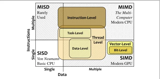
Figure 2.1: I categorize Instruction, Thread, Task, and Data-level Parallelism using Flynn’sTaxonomy

(SISD, MISD, MIMD, and SIMD). (Less importantly, I also categorize Vector- and Bit-level parallelism.)

Instruction-Level parallelism (ILP) executes instructions on multiple processing cores to increase the instruction throughput of a serial instruction stream. On CPUs, ILP has a huge effect on the underlying architecture, but thanks to the heroic efforts of hardware architects and

compiler writers, most programmers see little effect on the common programming model, and can continue to think of and work with modern CPUs as if they were simple von Neumann SISD computers instead of the complex MIMD systems on a chip (SoC) that they have become.

Thread-level parallelism (TLP), also known as multi-threading, maps multiple streams of execution onto multiple cores. Initially, multi-threading appears to be clearly in the MIMD category for both the architecture and the programming model. In fact, some of the first uses of TLP was to hide latency on SISD CPU architectures by switching from stalled threads to other active threads to continue doing useful work. On SIMD processors, batches of threads (known as warps on NVIDIA GPUs) are mapped onto batches of simple processing cores.

TLP enables task-level and data-level parallelism. Task-level parallelism divides one large task into several smaller subtasks and maps each subtask onto its own thread or warp. Data-level parallelism (DLP) partitions a large data set into smaller runs of data and also maps

(44)

16

each run onto its own thread or warp. I also show two other types of parallelism (bit-level parallelism (BLP) and vector-level parallelism (VP) that will I will revisit in my case study on Histograms (chapter 8).

See the book Computer Architecture5_{(Hennessey and Patterson, 2012), for a more} in-depth description of each type of parallelism above (as well as other types of parallelism).

2.1.2 Machine Models, Memory Models, and the Memory Hierarchy

Serial Model

von Neumann Machine

Parallel Model

The Multi-computer

Figure 2.2: Serial machine model vs. Parallel machine model. The classic serial von Neumannmodel

abstracts a sequential CPU plus a load/store memory that contains both instructions and data. The Multi-computer model abstracts parallelism by connecting multiple serial computers together via a network and adding support for remote message passing and remote memory access.

Flynn’s taxonomy includes data and instruction streams but does not cover types of memory access. Yet as we will see in my case studies, useful models of memory access are also important to GPU programmers in order to achieve take advantage of the performance

characteristics and features of the GPU memory hardware. Two machine models for thinking about instruction, data, and access parallelism are the von Neumann computer (von Neumann, 1945) and the multicomputer, shown in Figure 2.2. Machine models abstract hardware for programmers so that they can focus on high-level algorithms, data-structures, and

implementations without getting mired in the technical details of each machine’s specific architecture.

5_{For more information about different types of parallelism, see the book}_{Computer Architecture: A} Quantative Approach, 5th_Edition_{by Hennessey and Patterson.}

CPU Memory Input Zeta Smith Hernandez Brown … Output Allen Ashton Barlow Brown … Program

… Machine 1

(45)

17

The original machine model is the von Neumann computer, which consists of one CPU performing serial computations. The CPU connects to a storage unit called memory. All programs and data are stored in memory. Instructions and data are transferred between CPU registers and memory using load/store operations. The CPU executes a program containing a sequence of instructions to transform input data into output results.

The multi-computer contains a number of simple von Neumann computers called nodes that are linked to each other over an interconnection network. Each node executes its own program. Each program may access its own local memory directly. Each node may communicate and coordinate with other nodes over the network by sending and receiving messages. These simple abstract models have performed well for over sixty years by allowing advances in software to proceed independently from advances in hardware.

Under Flynn’s Taxonomy, a von Neumann machine is SISD, and the multicomputer is MIMD. For serial programming, programmers follow the random access memory (RAM) model and assume memory access costs are fixed regardless of the machine’s physical location.

For parallel programming, there are two main memory models: distributed memory and shared memory6_{. For distributed memory, programmers explicitly use remote message passing} over the interconnect network to communicate and coordinate parallel CPU nodes. In the ideal distributed model, message costs are proportional to message length. However, in practical models, message costs are impacted by three factors: 1) the topological layout of the network (meaning, cube, star, ring, etc.), 2) the physical distance between nodes, and 3) the number of messages competing for concurrent use of the interconnect network.

For the shared memory model, a large shared memory pool replaces the interconnect network. This model supports a concurrent RAM model. With it, every node has a direct

6_{Shared memory}_{is a general term in the parallel programming community for accessing memory in}

(46)

18

connection to the shared memory pool that all nodes share. Each node also has direct access to its own attached local memory pool. Because of communication overhead, access to other nodes shared memory is slower than direct access to its own local memory. The number of nodes involved in this model tends to be small, often 2 to 8, because the all-to-all communication required to support concurrent coherent access to shared memory grows geometrically as node are added.

In this shared memory context, coherent access implies that all changes to memory by any node are visible to all other nodes in the multicomputer. Programmers can implicitly use shared memory to communicate data and coordinate execution across parallel nodes. The

concurrent RAM model is easy for most programmers to understand since it is most similar to the RAM model they are already familiar with. However, concurrency implies that multiple nodes can update the same memory locations at the same time leading to resource competition. Programmers must prevent or manage resource competition between nodes to avoid serious problems, such as incorrect results and crashes.

Computer architects design and build memory architectures that are far more complex than the simple abstract models (RAM and concurrent RAM) programmers use to understand them. Because different memory technologies have many orders of magnitude differences in how they make trade-offs between cost, speed, and capacity, architects build large memory

hierarchies, both architects and compiler writers try to hide the hierarchy and simulate the simpler memory models for the average programmer. Because, in my case studies, the memory hierarchy of the GPU has a large effect on the techniques to improve performance, I want to review some of the terminology and issues in modern memory architectures.

(47)

19

stored in a slower memory level, move and store that variable into a faster memory level, a process called caching. Caching is effective because if an algorithm just accessed a memory location, that algorithm is likely to access the same location again soon, a concept called temporal locality. While the memory system is transferring data, it should also go ahead and grab a small fixed size neighborhood of memory around the requested memory location and cache that as well. Because if an algorithm just accessed a memory location, then that algorithm is likely to access that location’s neighbors as well, a concept called spatial locality. Frequently accessed memory ends up being cached in higher speed memory closer to the CPU resulting in better I/O

(48)

20

Figure 2.3 Memory Hierarchy with 4 broad tiers – very fast CPU registers, fast on-chip cache, medium speed off-chip RAM, and slow external file-based storage. Memory is typically sorted by access speed with fast memory kept close to the CPU and slow memory kept more distant. Architects use a memory hierarchy, caching, and the principle of locality to support fast average access speeds at a reasonable total cost.

Architects design modern computer memory in a hierarchical manner, as shown in Figure 2.3, to provide fast memory access at low cost. A typical memory system consists of four broad layers. The CPU layer consists of registers used to store input operands and output results. This memory is very fast but very expensive so designers keep it very small. The on-chip multi-level cache layer exploits locality by temporarily storing larger fixed size chunks of instructions and data. This memory is fast but expensive so it is kept small. The off-chip main memory layer consists of large amounts of random access memory (RAM) shared across all cores on the chip. This memory is reasonably fast, and affordable so it is kept large [1-32 GB]. Finally, the storage layer typically consists of file-system based hardware stored externally in devices such as USB keys, SSDs, DVDs, and hard drives. This memory is slow but cheap so designers can afford huge amounts of storage.

In theory, the RAM model treats memory access as having a fixed cost to make it easier to develop new algorithms. CPU architects and compiler writers put in great efforts to provide an

File Based Storage

External

SSD, Hard-drives, DVD, Tape, …

Main Memory

Off-chip

Random-Access Memory (RAM)

Cache

On-Chip L1, L2, L3, …

CPU

Registers

Fast,

Small,

Expensive

(49)

21

environment that most programmers can see as following the RAM model (at least if they respect some heuristics about accessing data with good locality, and partitioning drives wisely).

However, serial CPU programmers for whom performance is crucial may need to know much more about the memory hierarchy and may even circumvent some of the architects’ efforts by memory mapping or by using other tricks that operate on lower levels of abstraction. Currently, GPUs have less architecture and compiler support for the concurrent RAM model. So, in

practice, parallel GPU programmers have to much more aware of the memory hierarchy, memory types, and varying costs for accessing memory at each level.

2.1.3 Deriving a GPU core from a CPU core

The following diagrams shows the broad differences between CPU and GPU

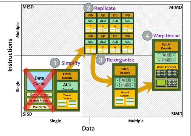
architectures, it summarizes a PPAM7_{tutorial by Göddeke (Göddeke et al, 2011). It shows how} to evolve a CPU into a GPU in four steps: simplify, replicate, re-organize, and warp-thread.. I place these in their categories in Flynn’s taxonomy in Figure 2.4.

At a high level, CPUs contain a few (2-8) large and complex ILP focused cores that favor coarse-grained Task-Level parallelism, whereas GPUs contain hundreds of simple TLP focused cores that favor fine-grained data-Level parallelism. This differentiation can be seen as arising naturally from the following steps.

7_{This summary is based on a}_{Parallel Processing and Applied Mathematics}_{(PPAM 2011) tutorial session}

(50)

22

Figure 2.4: Conceptual differences between a CPU core and a GPU core in broad themes. Based on a talk by Göddeke (Göddeke et al, 2011). Start with a complex CPU ILP-focused core. 1) Simplify: Remove complex ILP and large data caches to get a simple processing core. 2) Replicate: Repeat that simple core many times on the GPU chip to support massive parallelism. 3) Re-organize: Combine control logic for many simple cores into one larger single vectorized SIMD core. 4) Warp-thread: Support multi-threading at a group level, provide large context pools and hardware support for rapid context switching between groups of threads called warps. Finally, arrive at a GPU TLP-focused core.

Simplify:

The CPU is conceptually reduced to its essential functions for executing programs, keeping the fetch/decode control logic, an arithmetic logic unit (ALU) for

computation, and some execution context pools to support multi-threading. What is eliminated to save transistors is the large on-chip caches and most of the complex logic used to implement instruction-level parallelism (ILP) techniques. These simple cores will of course run slower than modern CPUs as they do not exploit serial parallelism or memory locality.

Replicate:

The saved transistors are then spent on creating many parallel simple cores on a single chip. To support parallel processing properly, control logic to schedule multiple threads onto multiple cores would also need to be added. This MIMD approach can support both

Data

Inst

ructio

ns

Single Multiple S ingl e Mult ip le Fetch/ Decode ALU (Execute) Thread Context Data Cache Out-Of-Order Branch Predict Pre-fetch

Simplify

MISD

_Replicate

MIMD

(51)

23

task-level and data-level parallelism. Algorithms that divide tasks or data across multiple cores will see a large performance gain due to parallelism.

Reorganize:

The core architecture is redesigned by reorganizing all of the ALU cores and their execution contexts into larger resource pools. To simplify yet further, a single instance of the instruction, control, and scheduling logic is shared across all the pooled ALU cores. This reduces the total transistor count at the cost of requiring all simple cores to move in lock-step through the same instruction stream. This approach is similar to vector-parallel computing and is at the heart of SIMD processing. For now, I will call this larger pooled core a SIMD core. This approach reduces system overhead by amortizing the cost of managing the instruction stream across many simple cores. Each simple core within the larger SIMD core works on the same instruction but on different data values, which strongly favors data-parallel algorithms.

Warp-thread:

Support is added for a large number of execution contexts for multi-threading in batches of threads. Using NVIDIA’s terminology, this batch of threads is known as a warp. Warp-threading allows the GPU to store a large number of dynamic warps and the associated state (or context) for each individual thread within each warp and additional context at the warp level. Each warp context corresponds to a batch of contexts (one per simple core) on the SIMD core. Think of warp-threading as multi-threading that occurs at the SIMD core level, not at the ALU core level with each warp-thread acting as a fat bundle of smaller threads (one per ALU core) that all move in lock-step through the instruction stream. All simple threads within a warp thread share a single warp context, including a program counter and other related resources (such as instruction cache or assigned shared memory) to march through the same instruction stream as a group.