A NEW APPROACH VERSUS BENDERS’
DECOMPOSITION IN AGGREGATE PRODUCTION
PLANNING
M. B. Aryanezhad
Department of Industrial Engineering, Iran University of Science and Technology Tehran, Iran, [email protected]
H. Mohammadi
Department of Industrial Engineering, Tehran South Unit, Islamic Azad University Tehran, Iran, [email protected]
(Received: November 30, 1998 – Accepted in Revised Form: May 3, 2001)
Abstract This paper proposes a simplified solution procedure to the model presented by Akinc and Roodman. The Benders’ decomposition procedure for analyzing this model has been developed, and its shortcomings have been highlighted. Here, the special nature of the problem is exploited which allowed us to develop a new algorithm through surrogating method. The two methods are compared by several numerical examples. Computational experience with these data shows the superiority of the new approach. In addition, the required computer programs have been prepared by the authors using TURBO PASCAL 7.0 to execute the algorithm.
Key Words Aggregate Production Planning, Benders’ Decomposition, Surrogating Method
ﻩﺪﻴـﻜﭼ
ﻩﺪﻴـﻜﭼ
ﻩﺪﻴـﻜﭼ
ﻩﺪﻴـﻜﭼ
ﺩ ـﻳﺍﺭ ﻪﻣﺎﻧﺮﺑﺭﺩﻦﻣﺩﻭﺭﻭﻦﻴﻛﺍﻪﻠﺌﺴﻣﻞﺣﻱﺍﺮﺑﻩﺩﺎﺳﻞﺣﺵﻭﺭﻚﻳﻪﻟﺎﻘﻣﻦ ﻪﺋﺍﺭﺍﻲﻣﺎﻏﺩﺍﺪﻴﻟﻮﺗﻱﺰﻳﺭ
ﺩﻮﺷﻲـﻣ .
ﺭﺮﺑﺩﺭﻮﻣﻝﺪﻣﻦﻳﺍﻞﻴﻠﺤﺗﻱﺍﺮﺑﺯﺭﺪﻨﺑﻪﻳﺰﺠﺗﺵﻭﺭ
ﺺﻗﺍﻮﻧﻭﺖﺳﺍﻪﺘﻓﺮﮔﺭﺍﺮﻗﺩﺪﺠﻣﻲﺳ ﻱﺎﻫﺩﻮﺒﻤﻛﻭ
ﺖـﺳﺍﻩﺪـﺷﻊـﻗﺍﻭﺮـﻈﻧﺪﻣﻥﺁ .
ﻢﺘﻳﺭﻮﮕﻟﺍﻥﺍﻮﻨﻋﺖﺤﺗﻱﺪﻳﺪﺟﻢﺘﻳﺭﻮﮕﻟﺍﻪﻛﺪﺷﺚﻋﺎﺑﻪﻠﺌﺴﻣﻦﻳﺍﺹﺎـﺧﺖـﻌﻴﺒﻃ
ﺩﻮـﺷﻪـﺋﺍﺭﺍﻲﻨﻴـﺸﻧﺎﺟ .
ﺎﺴﻣﻞـﺣﻂـﺳﻮﺗﺵﻭﺭﻭﺩﺮـﻫ ﺋ
ﺪﻧﺍﻪﺘﻓﺮﮔﺭﺍﺮﻗﻲﺳﺭﺮﺑﺩﺭﻮﻣﻒﻠﺘﺨﻣﻱﺩﺪﻋﻞ .
ﻦﻳﺍﺞﻳﺎﺘﻧ
ﻥﺎﺸﻧﺍﺭﺪﻳﺪﺟﻢﺘﻳﺭﻮﮕﻟﺍﻱﺮﺗﺮﺑﺕﺎﺒـﺳﺎﺤﻣ
ﺪﻫﺩﻲﻣ . ﺑ ﺯﺎﻴﻧﻱﺩﺪﻌﺘﻣﻱﺮﺗﻮﻴﭙﻣﺎﻛﻱﺎﻫﻪﻣﺎﻧﺮﺑﻪﺑﻖﻴﻘﺤﺗﻦﻳﺍﺭﺩﻩﻭﻼﻌ
ﻪﻛﺩﻮﺑ ﺯﺍﻩﺩﺎﻔﺘﺳﺍﺎﺑﻪﻟﺎﻘﻣﻥﺎﮔﺪﻨﺴﻳﻮﻧﻂﺳﻮﺗ ﻝﺎﻜﺳﺎﭘﻮﺑﺭﻮﺗ
) ﻢﺘﻔﻫﺖﻳﺍﻭﺭ (
ﺪﻧﺍﻩﺪﺷﻪﺘﺷﻮﻧ .
INTRODUCTION
Aggregate Production Planning (APP) is an intermediate range production problem (the planning horizon is generally three months to two years), in which one attempts to achieve a (cost– effective) balance between productive capacity, on one hand, and forecasts of fluctuating demand, on the other. The production manager typically has at his disposal a set of production options with which to achieve the balance. Despite the strong interest that has been shown in APP models reported examples of successful implementation have been rare [1]. Akinc and Roodman [1,2], first suggest several reasons for this failure, and then introduce a mixed integer-programming model for aggregate
production planning that attempts to address the limitations they have listed. The reformulation of APP by Akinc and Roodman may be seen in the modeling framework of this paper.
Bender’s decomposition [3] is a well-known constraint generation approach for problems where certain variables make the problem more difficult, for example Mixed Integer Linear Programming (MILP) problems that is the nature of the problem here. A disadvantage of this approach is that the Benders’ master problem is often very hard to formulate which can make the method inefficient. Possibilities of solving the Benders master problem by speeding up the procedure have been dealt with by, for example, Cote and Laughton [4].
version of Benders’ decomposition for analyzing this model. The salient features of this complicated procedure are listed in [1]. For complete description, the reader is referred to Akinc and Roodman [2].
Various papers, e.g. Paula jr. and Maculan [5] and Rana and Vickson [6] use Benders’ decomposition with Lagrangean relaxation applied to the Benders’ cuts [3] in the master problem. Diaby [7] presented an implicit enumeration procedure for solving pure integer 0/1 minimax problems, which arise in the context of Benders’ decomposition for mixed integer 0/1 linear programming problems.
However, Holmberg [8] gave some small counter examples of MILP problems, which this approximations (of Benders’ master problem), fails to solve, i.e. yields bounds worse than the LP relaxation or even fails to find any feasible solution.
Aryanezhad [9] proposed a new algorithm for solving a special version of this aggregate production planning with zero-one variables. In this procedure the master problem of the APP was not an optimization problem, but the subproblems were basically transportation models. The transportation structure of subproblems, and the non-optimal nature of the master problem, made the new approach quite superior to the previous mixed integer programming routines.
A branch and bound method based on a dual ascent and adjustment procedure is developed by Holmberg [10] and compared to application of a modified Benders’ decomposition method.
In this paper the full model of APP has been reconsidered and a new algorithm is proposed. The procedure we propose for analyzing this MILP model is a modified version of Benders’ decomposition that exploits the intricacies of both the restricted master problem and the related subproblems. Here, the restricted master problem will be developed by surrogating method (Glover [11]) that is a binary variable problem (BVP). We will show that the optimal solution of this BVP is straightforward. This result and the proposed incumbent solution to initiate the new approach will speed up the procedures. In order to show the superiority of the new algorithm the authors developed all the required programming codes through TURBO PASCAL 7.0 for Gomory’s all
integer dual method [12], Balas zero-one additive algorithm [13], strongest surrogate constraint [11,14], Benders’ decomposition [3] and so on. Several numerical examples have been generated and solved by the new algorithm and Benders’ decomposition. The results are tabulated and the execution time and number of iterations have been compared.
THE MODELING FRAMEWORK
To state the model, it is useful to distinguish between two types of production strategies, which we shall call production modes (PM), and capacity adjustments (CA). Production modes will refer to the alternative methods that can be used to produce units of output. They will be distinguished from one another by their cost structures and/or the technology that they employ. Typical production modes would include regular time scheduling, overtime scheduling, use of a more labor-intensive production method, subcontracting, substitution of lower quality raw materials, etc. Capacity adjustments, in contrast, will refer to the choices that determine the levels at which the production modes operate. Capacity adjustments might include changing the size of the workforce, activating idle equipment, re-scheduling preventive maintenance, etc.
In the model that follows, a binary variable, yikt will be used to denote whether the kth CA is used with mode “i” in period “t”. In order to avoid introducing additional variables, we will denote the use of a mode “i” in period “t” by yi1t, (the first CA). The function of properly counting any mode-related fixed costs will be performed by yi1t. To illustrate the relationship between yi1t, and yikt, k≠1, consider overtime production as mode “i” which can be scheduled in two increments with known capacities 6-8 P.M. weekday program or a weekend program. One would model this situation by representing the existence of any overtime production by yi1t and the two CA’s by yi2t and yi3t. Constraints:
yi1t≥ yikt and k = 2,3
a capacity adjustment of zero but it represents a precondition for the use of CA’s.
In some cases, a mode may be associated with a primary CA. For example, in regular time production, the capacity due to the existing work force has priority over any CA’s due to hiring programs; likewise, in subcontracting there may be a preferred supplier who is resorted to first before any other supplier (CA’s) is activated. In such cases, the capacities of these priority adjustments can simply be associated with the variable yi1t. This scheme of representing modes and CA’s gives a certain degree of modeling flexibility, whereby the overall capacity level can be represented by a y-vector:
y = < yikt>
The model can be stated as follows: Minimize:
∑ ∑ ∑
∑ ∑ ∑
= − = = + = = =+
+
+
T 1 t ikt ikt M 1 i ikt ikt K 1 k ikt ikt T 1 t M 1 i T 1 it it)
Z
b
y
f
Z
a
(
X
C
itl l l
Subject to:
T
,...,
1
t
M
,...,
1
i
)
y
(
R
X
it T 1 it=
=
≤
∑
=l l (1)
T
,...,
1
t
M
,...,
1
i
)
y
(
L
X
it T 1 it=
=
≥
∑
=l l (2)
1 T ,..., 1 F X T 1 t it M 1 i + = ≥
∑
∑
== l l l
(3)
T
,...,
1
t
K
,...,
1
k
M
,...,
1
i
)
Z
Z
(
y
y
it T 1r ikr ikr
0 ik ikt
=
=
=
−
+
=
∑
= − + (4)yikt≤ yi1t i = 1,…,M
k = 2,…,Kit (5) t = 1,…,T
Linear Configuration Constraints on y including those representing desired end conditions.
Xitl≥ 0 (6)
yikt, Z+ikt, Z−ikt = 0,1 where
M = the number of production modes, T = the number of time periods,
Kit = the number of capacity adjustments for production mode “i” in period “t”,
Fl = forecast demand in period “l” (FT+1 desired ending inventory level),
Citl= the variable cost to produce one unit of output using production mode “i” (regardless of its capacity level) in period “t” to meet demand in period “l”.
Xitl= the number of units produced using production mode “i” in period “t” to meet demand in period “l”,
aikt = the fixed cost to first establish capacity adjustment “k” for production mode “i” at the beginning of period “t”,
bikt = the fixed cost to remove capacity adjustment “k” for production mode ”i” at the beginning of period “t”,
fikt = the fixed cost to operate capacity adjustment “k” for production mode “i” in period “t”,
Z+ikt= 1, if capacity adjustment “k” for production mode “i” is started at the beginning of period “t”, 0, otherwise,
yikt = 1, if capacity adjustment “k” for production mode “i” is in use during period “t”, (yik0 initial condition) 0, otherwise,
Ζ−
ikt = 1, if capacity adjustment “k” for production mode “i” is removed at the beginning of period “t”, 0, otherwise,
Rit(y)= the capacity of production mode “i” in period “t” (a linear function of y), and Lit(y)= a lower bound on output of production
In general, additional production modes will lead to additional constraints in the framework, where as additional capacity adjustment will change the form of the Rit (y) and Lit (y).
Constraints 1 specify that total production cannot exceed available capacity for each mode in each period, while Constraints 2 establish minimum quotas on total production for each mode in each period. Constraints 3 require that demand be met in each period (although they do not necessarily preclude back-ordering). Then (4) specifies the relationship that must exist among “start-up”, “shut-down”, and “operating” variables for each production mode and/or capacity adjustment (Z+ikt, Z−ikt and yikt, respectively). Finally, constraints (5) as discussed earlier, require that the mode “i” is in place before any further capacity increment can be employed.
The constraints in (6) are those which might be required, depending on the particular problem characteristics, to establish logical relationships among PMs and, CAs as well as desired end-of the period conditions for PMs and CAs.
MODEL ANALYSIS
Surrogating Method
Here, we show that the main constraints of the master problem will be replaced by the strongest surrogate constraint. The surrogate constraints are the non-negative linear convex combinations of the main constraints and the objective function [11,14]. The generated problem with the strongest surrogate constraints is a valid relaxation of the main problem with zero-one variables.DEFINITION 1: Suppose Ay ≤ b is the constraints of a special problem. Suppose V≥ 0 is given. Then the surrogate constraint for this problem is VTAy ≤ VTb, [11,14].
DEFINITION 2: Suppose the objective function of a given problem is a minimization problem. Suppose there exists at least two surrogate constraints the strongest surrogate constraint is the one, which implies less value for the objective function.
Consider a linear mixed integer programming
with zero-one variables: Min dx + cy
S.t. Dx + Ay ≥ b (MIP )
1 ≥ y ≥ 0 (MIP) x ≥ 0
y integer
The dual of (MIP) for a given y =
y
is Max U0 = U (b-Ay
)S.t. UD ≤ d U ≥ 0 Let us define:
Suppose
U
ki is an extreme point of the following constraint (1) for all i=1,2,…,|K|.{UD ≤ d, U ≥ 0} (1) Now, the integer problem of Benders’ decomposition (1962) is as follows:
Min Z
S.t. Z ≥ cy + UkT (b-Ay), k=1,2,...,p (IP) 1 ≥ y ≥ 0 and integer
Then in terms of this notation, any Benders’ integer subproblem like (IP) can be formulated as follows:
Min Z
S.t. Z1 ≥ (1c) y + UKT(b-Ay) (BIPK) (BIPK) 1 ≥ y ≥ 0
y integer
Suppose VK ≥ 0 is a given vector, then the surrogate constraint for (BIPK) can be written as: VKT(1Z) ≥ VKT(1c) y + VKTUKT(b-Ay) (2) Then, the strongest surrogate constraint for zero-one variables y, which maximizes VK≥ 0 will
{
1,2,...,p}
P , P K , K k ,..., k , k
), U ,..., U , U ( U
K 2 1
k k k
K 1 2 K
be:
Max{Min{[VKT1]-1[VKT(1c) y+VKTUKT (b-y)]}} (3) VK≥ 0 y = 0,1
Since VK’s are the convex combination vectors, therefore VKT1 should be equal to one, or VKT1=1. In other words (3) is equivalent to (4). Max {Min{[c-VKTUKTA] y + bT(UKVK)}} (4) VK ≥ 0,VKT1=1 y = 0,1
Since y is a binary variable, then optimization of the relationship inside bracket in (4) is straightforward. In the other words:
1, if (c- VKT UKT A) i < 0, yi =
0, otherwise.
Now, let us define a new vector W such as Wj = max {0, -(c- VKT UKT A) j}.
Then, (4) may be changed to a linear programming model with the help of new vector W. That is,
Max bT UK VK – 1TW S.t. AT U
KVK – W ≤ c 1T V
K = 1 (BSPK)
VK, W ≥ 0
The optimal solution of (BSPK) would imply (
V
K), to be the strongest surrogate constraint for Benders integer programming (BIP).Now, let us consider (BIPK), and write its dual problem:
Max bT U
K VK – 1TW S.t. 1T V
K =1 (5) ATUKVK – cT VK – W ≤ 0 (6) VK, W ≥ 0
Since 1T V
K=1, Then, cT VK =1(cT VK)=(1cT) VK= (c1T) V
K = c (1T VK) = c, the Constraint 6 will be replaced by (7):
AT U
K VK –W ≤ c (7) Therefore, the dual of (BIPK) will be as
follows: Max bT U
K VK - 1TW S.t. AT U
K VK – W ≤ c 1T V
K = 1 (DBIPK)
VK, W ≥ 0
Here, we see that (BSPK) and (DBIPK) are the same. In other words, the optimal solution of the dual problem of (BIPK) would imply
V
K which is the strongest surrogate constraint for (BIPK). Therefore, the strongest surrogate constraint would be as follows:Z ≥ cy +
V
KUKT (b-Ay) (8)Trivial Solution of (BIP
) The biggest obstacle associated with Benders’ decomposition is the solution of master problem. However, the special structure of the APP problem in conduction with the strongest surrogate constraint method, make the master problem to have one constraint with zero-one variable. So, in each iteration, we have the following optimization problem:Min Z
S.t. Z ≥ (c - A) y + b y = 0,1
The optimal solution of this problem is straightforward. Hence,
1, if (c - A) i < 0, yi =
0, otherwise.
The Initial Solution
Let us consider Benders’ final integer programming when all of the constraints are generated:Min Z
S.t. Z ≥ cy + UPT(b-Ay) (BIPP) (BIPP) 1 ≥ y ≥0
y integer
the dual problem of (BIP P). Max bT U
P VP – 1TW S.t. AT U
P VP – W ≤ c
W ≥ 0 (BSPP)
1T V P = 1 VP≥ 0
The strongest surrogate constraint would be: Z ≥ cy + (UPVP*)T(b-Ay) (9)
Let us write the dual problem of MIP , which is:
Max bTπ -1Tα S.t. ATπ - α≤ c
α≥ 0 (DMIP )
DTπ≤ d π≥ 0
Now, let us prove that (DIMP ) and (BSPP) are equivalent.
Theorem
. (VP*, W*) is an optimal solution for (BSPP), if and only if π* =UPVP* & α* = WP* is an optimal solution for (DMIP ).Proof
. The objective function and the first two constraints will be the same if we do the desired transformation. The remaining constraints will be the same if we show that the two sets of (10) and (11) are equivalent.DTπ≤ d (10)
π≥ 0 1TV
P =1 (11)
VP≥ 0
The set (10) is always feasible and bounded. So, if we suppose that π = UP VP is its vertices then the linear convex combination of its vertices is also its solution. Therefore, (11) is satisfied. Conversely, suppose (11) is true. Then by reconsidering (11) we have,
DTU P≤ d
UP≥ 0 (12)
Multiplying (12) by VP ≥ 0 and summing it up, we will have DTU
PVP≤ d (1VP). Since (1VP) =1, then
DTU
P VP≤ d (13)
By considering the transformation π= UPVP in (13) we have DTπ≤ d.
Since VP≥ 0 and UP≥ 0 then π= UPVP ≥ 0 and the proof is complete.
If (π*, α*) solve (DMIP ), then the strongest surrogate constraint for (BIPP) will be as follows: Z ≥ cy + π* (b-Ay).
Then the trivial solution of the following surrogate integer problem (SIP) will yield
y
. Thisy
will be an initial value for starting the new algorithm. The objective value of Z will be a lower bound for the objective value of MIP.Min Z
S.t. Z ≥ cy + π* (b-Ay) (SIP)
y =0,1
THE NEW ALGORITHM
In this section we are in a position to introduce a new algorithm based on the above analysis. We will also mention some properties, which reduce the computational efforts.
Step 1 (Initialization): Solve the linear program (DMIP ) and derive π*. Then derive the straightforward binary solution of (SIP) and call it
y
.Put Z = Zl , Zu = +∞, and k=1. GO TO STEP 2.
Step 2: Solve the following linear program: Max U0= U (b-A
y
)S.t. UD ≤ d U ≥ 0
Put
U
k←
U. Then update Zu =min {Zu, UStep 3: Construct the main constraint Z ≥ cy +Uk(b-Ay) with the help of Uk in step 2. If this inequality is a redundant constraint, then GO TO STEP 6. Otherwise, GO TO STEP 4.
Step 4: Suppose K=
{
1
,
2
,...,
k
}
. If k=1 thenV
K=1 and GO TO STEP 5.Otherwise solve (DBIPK). Find the optimal VK. Then put
V
K←
VK, and GO TO STEP 5.Step 5: Construct the strongest surrogate constraint as the following:
Z ≥ cy +
V
KUKT (b-Ay)For k=1 this constraint is unique. Develop the surrogate integer problem (SIP) as follows:
Min Z
S.t. Z ≥ cy +
V
KUKT (b-Ay) (SIP)y =0,1
The optimal solution of (SIP) is straightforward:
−
<
=
.
otherwise
,
0
,
0
)
A
U
V
c
(
if
,
1
y
iT K T K i
Put
y
equal to the optimal y. Ify
is a repeating value, then GOTO STEP 6. Otherwise, find Zl = cy
+ TK
V
UKT (b-Ay
) and GO TO STEP 7.Step 6: Solve the following integer program: Min Z
S.t. Z ≥ cy +Ui (b-Ay), i = 1,2,…,k
y =0,1
This is the only integer programming problem that should be solved only once in this new approach. Put
y
equal to the optimal value of y, and Zl = min Z. Then GO TO STEP 7.Step 7: If Zl < Zu, then k←k+1 and GO TO STEP 2.
Otherwise, Zl =Zu and
y
is the final optimal y. For finding the final optimal x, solve the following linear programming problem.Min dx S.t. Dx ≥ b-A
y
x ≥ 0Then x =
x
, y =y
, Zl = Zu = dx
+ cy
are the final optimal solution of the original MILP.NUMERICAL EXAMPLE
For purposes of illustration, we have solved several examples based on the example given by Akinc and Roodman [1]. One of the illustration problems has the following parameters:
There is a three period planning horizon with forecast demands of 800, 950, 1250 units of output. Production data is summarized below: 1. Regular Time Workforce. Initial regular work force is 20 workers where each worker contributes 35 units to output. An additional increment of 10 workers is available. Hiring/firing and incremental payroll costs associated with this option are $400, $250 and $700 per worker, respectively.
2. Overtime. Actual overtime production is restricted to no more than 20% of regular time production. With this constraint, the company can employ overtime increment at capacity of 70 units/period. The variable overtime penalty is $6 per unit for the overtime increment. In addition, there is a $30/period incremental fixed overhead expense.
3. Inventory-Backlog. Inventory carrying cost is $5/unit/period while demand can be backlogged at a cost of $20/ unit/period.
In order to represent this problem within the framework given earlier, we may define production modes of (1) regular time, (2) overtime, and hiring-firing, as capacity adjustment to regular time production. The following zero-one variables will be required to model these:
Mode 1.Regular Time Production Adjustment:
Mode 2. Overtime Production Adjustment:
Overtime Increment (Use/Not Use) y21t The cost parameters for the problem will be as follows:
Inventory/ Backlog/ Operating
5 (l - t) l≥ t C1tl =
20 (t - l) l < t
6 + 5 (l - t) l≥ t C2tl =
6 + 20 (t - l) l < t
Hiring/Firing
a11t = 400, all t (hiring)
f11t = 700, all t (additional payroll, etc.) b11t = 250, all t (firing)
Overtime
a21t =0, all t f21t =30, all t b21t =0, all t
The Model
. The model is then Minimize:∑
∑
∑
= −
=
+
+
+
+
+
3 1 t 21t t
11
t 11 3
1
t 11t it
3 , 3 , 2
, t ,i it
y
)
Z
250
y
700
Z
400
(
X
C
ll l
Subject to:
(Labor Hrs.) 11t
3 1 1t
y
350
700
X
≤
+
∑
=
l l
, all t
(O.T. Cap) 21t
3 1 2t
y
70
X
≤
∑
=
l l
, all t (O.T. Limit) 70y21t ≤ 0.20(700+350y11t), all t
∑
=
−
+
−
=
t1
r 11r 11r t
11
(
Z
Z
)
y
, all t∑
2,3≥
t ,i it
F
X
l l, all lXikt ≥ 0, yikt, Z+ikt, Z−ikt = 0,1
Optimal Solution. The optimal solution of this problem in summary form is to schedule overtime production mode in period 3, and to hire 10 workers in period 1 and let them work in periods 1-3. The cost of this solution is $3750 consisting of $1220 of variable (inventory, backordering, overtime penalty) and $2530 of fixed costs (hiring, firing, and fixed wages of 10 employees, and incremental overhead due to overtime).
This problem was solved by Benders’ decomposition technique, through solving four linear programming problems and four integer-programming problems. However, the new approach solved this problem by solving ten linear programming problems, but one integer programming.
COMPUTER PROGRAMMING CODES
To compare, the new approach and Benders’ decomposition technique, the authors prepared the following computer programming codes through TURBO PASCAL 7.0.
1. Revised Simplex Method. 2. Dual Simplex Method.
3. Gomory All integer Dual Method. 4. Balas Zero-one Additive Algorithm. 5. Strongest Surrogate Constraint Method.
COMPUTATIONAL EXPERIENCE
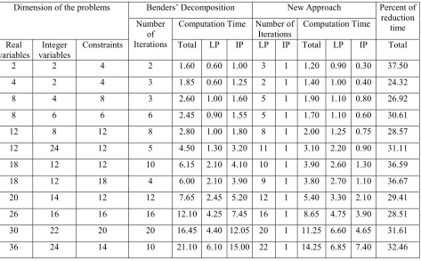
TABLE 1. Comparison of Time reduction in the New Approach with Respect to Benders’ Decomposition.
These problems were solved by Benders’ decomposition and by our New Approach (NA) on a 486 DXII computer with 8MB Ram. The dimensions of the problem, number of iterations, time of computation, number of LP and IP, and percent of computational time reduction of the NA with respect to the Benders’ decomposition are tabulated in Table 1. In this table we can see that computation time of the new approach is smaller than Benders’ decomposition algorithm. The number of integer program problems in the new approach was always only one problem, while in the Benders’ procedures it varies with the number of iterations i.e., twenty integer program problems in the largest example.
CONCLUSION
In this research a new approach was developed for solving more flexible kind of aggregate production problems as formulated by Akinc and Roodman
[1]. Some of the advantages of the new approach compared with Benders’ decomposition procedure are listed below:
• Replacing the integer subproblems by linear problems.
• Reduction of the number of integer programming problem, to one.
• Generation of a good initial solution.
• Finding a good lower bound for the objective function in the first step of the NA.
• Reduction of the computational time.
The new approach was applied to the new formulation of aggregate production planning problem with zero-one variables. However, the application of the new algorithm for general mixed integer programming is an open question.
REFERENCES
1. Akinc, U. and Roodman, G., “A New Approach to Aggregate Production Planning”, IIE Transaction,
Benders’ Decomposition New Approach Dimension of the problems
Computation Time Number of
Iterations Computation Time
Percent of reduction
time Real
variables
Integer variables
Constraints
Number of
(1986), 88-94.
2. Akinc, U. and Roodman, G., “Dynamic Facility Location: The Phase-In/Phase-Out Case”, Working Paper, (1982). 3. Benders, J. F., “Partitioning Procedures for Solving Mixed
Variables Programming Problems”, Numerische Mathematik, Vol. 4, (1962), 238-252.
4. Cote, G. and Laughton, M. A. “Large-Scale Mixed Integer Programming: Benders-Type Heuristics”, European Journal of Operational Research, Vol. 16, (1984), 327- 333.
5. Paula, JR. and Maculan, N., “A P-Median Location Algorithm Based on the Convex Lagrangean Relaxation of the Benders Master Problem”, Presented at the 13th
International Symposium on Mathematical Programming, Tokyo, Japan, (1988).
6. Rana, K. and Vickson, R. G., “A Model and Solution Algorithm for Optimal Routing of a Time-Chartered Container Ship”, Transportation Science, Vol. 22, (1988), 83-95.
7. Diaby, M., “Implicit Enumeration for the Pure Integer 0/1 Minimax Programming Problem”, Operations Research, Vol. 41, (1930), 1172-1176.
8. Holmberg, K., “On Using Approximations of the Benders
Master Problem”, European Journal of Operational Research, Vol. 77, (1994), 111-125.
9. Aryanezhad, M. B., “A New Approach To Aggregate Production Planning with Zero-One Variables”,
Proceedings of the 1995 IFAC Symposium on Information Control Problems in Manufacturing In China, (1995), 381-388.
10. Holmberg, K., “Exact Solution Methods for Incapacitated Location Problems with Convex Transportation Costs”,
European Journal of Operational Research, Vol. 114, (1999), 127- 140.
11. Glover, F., “Surrogate Constraint Duality in Mathematical Programming”, Operations Research, Vol. 23, No. 3, (1975), 434-451.
12. Gomory, R. E., “An All-Integer Integer Programming Algorithm”, Chapter 13 in Industrial Scheduling, Prentice-Hall, Englewood Cliffs, New Jersey, 1963.
13. Balas, E., “An Additive Algorithm for Solving Linear Programs with Zero-One Variables”, Operations Research, Vol. 13, (1965), 517-546.