Numerical Solutions of the Regularized Long-Wave
(RLW) Equation Using New Modification of
Laplace-Decomposition Method
Nawal A. Al-Zaid, Huda O. Bakodah, Fathiah A. Hendi
Department of Mathematics, Science Faculty for Girls, King Abdulaziz University, Jeddah, KSA Email: [email protected], [email protected], [email protected]
Received July 28, 2012; revised September 30, 2012; accepted October 8,2012
ABSTRACT
In this paper the new modification of Laplace Adomian decomposition method (ADM) to obtain numerical solution of the regularized long-wave (RLW) equation is presented. The performance of the method is illustrated by solving two test examples of the problem. To see the accuracy of the method, L2 and L∞ error norms are calculated.
Keywords: Adomian Decomposition Method; Regularized Long-Wave (RLW); Laplace Transform
1. Introduction
The regularized long wave (RLW) equation which can be shown in the form
0
t x x xxt
u u uu u
(1) where , are positive parameters, is an important nonlinear wave equation. This equation plays a major role in the study of nonlinear dispersive waves. The RLW equation particularly describes the behavior of the undular bore [1-3], it has also been derived from the study of water waves and ion acoustic plasma waves.
The RLW equation has been solved analytically only for restricted set of boundary and initial conditions. There- fore, the numerical solution of this equation has been the subject of many papers [4-7]. Recently a great deal of interest has been focused on application of Adomian de- composition method (ADM) to solve a wide variety of nonlinear problems [8,9]. In this paper, we will apply the new modification of Laplace ADM to the RLW Equation (1). The soliton solution of RLW equation has the form
2
0
sech p x vt x
, 3
u x t c (2)
where pis an arbitrary constant and
1 22 1
c c
1
v c 1
1
p ,
, 0
, 0
u x f x
, and c is a constant [10]. In this
work, a new modification of Laplace ADM is used to solve the RLW equation with the initial condition
(3)
x is a localized disturbance inside the
con-sidered interval.
where
2. Description of Method
We begin by consider Equation (1) in an operator form
0t x
L u u R u N u
f
(4)
where Lt
t
is a linear operator and R its remainder
of the linear operator. The nonlinear term is represented by N u
t x
L u u R u N u
0
, n ,
n
u x t u x t
0
. Thus we get
(5) We represent solution as an infinite series given be-low,
(6) The nonlinear term Nu can be decomposed into
infi-nite series of polynomial given by:
x n
n
Nu uu A
, , , n u u u
0 0 0 1 0 1 1 0 2 0 2 1 1 2 0
x
x x
x x x
A u u
A u u u u
(7) where An are Adomian polynomials [11] of 0 1
and it can be calculated by formula given below:
u u u u u u
A
in a similar manner.
By applying the Laplace transform to both sides of Equation (5), we obtain
L ut
ux
Ru
Nu (8)Thus
,
1
,0 1
x
u x t u x u
Ru
Nu
s s
(9) In the new modification of ADM [12], Wazwaz re-placed the initial condition u x
,0
0, 0 n n u x
by a series of infi-nite components i.e.,
, 0u x (10)
and the new recursive relationship can be expressed in the form
0 0,0
1 0, 1
1
, ,0 ,
1
, ,0
1
n n
x
U x s u x
s
U x s u x
s
u Ru
Nu
,n 0s
0 , n nU x s
(11) where
u x t,
U x s
, (12)
Now, by applying inverse Laplace transformation we get:
, , , 0
x s
x s n
m u
0 , m m i iu u x t
u e
1 0 0 1 1 1 , , n nu x t U
u x t U
(13)
Using (13) the series solution follows immediately.
3. Numerical Examples and Results
In this section, the new modification of Laplace ADM will be demonstrated on illustrative examples and we compare the approximate solution obtained for our RLW equation with known exact solutions. We define to be m-term approximate solution, i.e.
e the exact solution and m the absolute error between
the exact solution and the approximate solution
m e m
e u u
In order to show how good the numerical solutions are in comparison with the exact ones, we will use the L2 and
L∞ error norms defined by
1 2 2
2 2 , ,
1 m
e m e i m i
i
L u u x u u
, , maxe m e i m i
i
L u u u u
Example (1)
We consider Equation (1) with the initial condition
20
,0 3 sech
u x c p xx
The exact solution of this problem is given by Equation (2). This solution corresponds to the motion of a single solitary wave with amplitude 3c and width p, initially
centered at x0, where v 1 c
1
is the wave velocity. We use the new modification of Laplace ADM to solve this equation, all computations are done for the parameters
0 0
x
,
1 and . 0.1
c
We consider , as in [13], so the initial condition
,0u x can expressed as a series of infinite components
i.e.
2 4
12
6 8 10
, 0 0.3 0.00681818 0.000103306
1.33045 1.5754 1.77355
u x x x
x x x O x
Using recursive relation (11) yield the components
1 1
0 0
0.3
, , 0.3
u x t U x s
s
1
1 21 1
2
0.00681818
, ,
0.00681818
u x t U x s x
s x
1
2 2
4
, ,
0.0177273 0.000103306
u x t U x s
tx x
1 3 3 2 3 6 6 , , 0.0115227 0.000630165 1.33045 10u x t U x s
t tx x
And so on, in this manner the rest of components of the decomposition series were obtained. The results are given in Table 1. The error norms for (c = 0.1) are
re-corded in Table 2 for different value of m.
Also in Figure 1 we show the exact solution and nu-merical solution with new modification of Laplace ADM for t = 0.1 and t = 0.5. Figure 2 shows the exact solution
and numerical solution with new modification for t = 0.5
at the interval 5 ≤x≤ 5. Example (2)
In the second test problem [14], a smaller solitary wave of amplitude 0.109 (c = 0.05), has been modeled.
The initial condition u x,0
can expressed as a se-ies of infinite components i.e.Table 1. Absolute errors for Example (1) with c = 0.1 and m = 10.
x/t 0.01 0.02 0.03 0.04 0.05
0.1 4.60152 × 10⁻⁷ 4.29123 × 10⁻⁷ 9.14459 × 10⁻⁸ 1.09975 × 10⁻⁶ 2.59382 × 10⁻⁶
0.2 1.15346 × 10⁻⁶ 1.8112 × 10⁻⁶ 1.97626 × 10⁻⁶ 1.65183 × 10⁻⁶ 8.41272 × 10⁻⁷
0.3 1.82435 × 10⁻⁶ 3.1446 × 10⁻⁶ 3.96518 × 10⁻⁶ 4.29071 × 10⁻⁶ 4.12595 × 10⁻⁶
0.4 2.4624 × 10⁻⁶ 4.40862 × 10⁻⁶ 5.84456 × 10⁻⁶ 6.77623 × 10⁻⁶ 7.20981 × 10⁻⁶
[image:3.595.58.541.224.520.2]0.5 3.05691 × 10⁻⁶ 5.58214 × 10⁻⁶ 7.58301 × 10⁻⁶ 9.06702 × 10⁻⁶ 1.00418 × 10⁻⁵
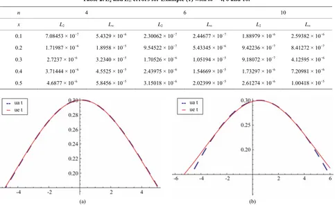
Table 2. L2 and L∞ errors for Example (1) with m = 4, 6 and 10.
n 4 6 10
x L2 L∞ L2 L∞ L2 L∞
0.1 7.08453 × 10⁻⁷ 5.4329 × 10⁻⁶ 2.30062 × 10⁻⁷ 2.44677 × 10⁻⁷ 1.88979 × 10⁻⁶ 2.59382 × 10⁻⁶
0.2 1.71987 × 10⁻⁶ 1.8958 × 10⁻⁵ 9.54522 × 10⁻⁷ 5.43345 × 10⁻⁶ 9.42236 × 10⁻⁷ 8.41272 × 10⁻⁷
0.3 2.7237 × 10⁻⁶ 3.2340 × 10⁻⁵ 1.70526 × 10⁻⁶ 1.05194 × 10⁻⁵ 9.18072 × 10⁻⁷ 4.12595 × 10⁻⁶
0.4 3.71444 × 10⁻⁶ 4.5525 × 10⁻⁵ 2.43975 × 10⁻⁶ 1.54669 × 10⁻⁵ 1.73297 × 10⁻⁶ 7.20981 × 10⁻⁶
0.5 4.6877 × 10⁻⁶ 5.8456 × 10⁻⁵ 3.15018 × 10⁻⁶ 2.02399 × 10⁻⁵ 2.61274 × 10⁻⁶ 1.00418 × 10⁻⁵
[image:3.595.55.540.233.512.2]
(a) (b)
Figure 1. The exact solution and numerical solution with new modification of Laplace ADM for Example (1), for t = 0.1 and (b) for t = 0.5.
(a) (b)
Figure 2. (a) The exact solution for t = 0.5 and −5 ≤ x ≤ 5; (b) Numerical solution with new modification for t = 0.5 and −5 ≤ x 5.
≤
[image:3.595.99.509.555.707.2]
210 8
,0 0.15 0.00178571 0.0000141723 9.56 5.93001 10
u x x
8
4 6
12
07 10
x
13 3
2 3
8 6
, ,
0.00236161 0.0000715703 9.5607 10
u x t U x s
t tx
x
x
x
x O
Using recursive relation (11) yield the components
11
u x t
0 , 0 ,
0.15 0.15
U x s
s
1
11 1
2
0.00
, ,
0.00178571
u x t U x s
x
178571x2
s
4
000141723x
1
2 , 2 ,
0.00410714 0.0
u x t U x s
tx
And so on, in this manner the rest of components of the decomposition series were obtained.
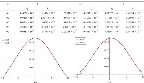
The results are given in Table 3 and the error norms for (c = 0.05) are recorded in Table 4 for different value of m. Also in Figure 3 we show the exact solution and nu-merical solution with new modification of Laplace ADM for t = 0.1 and t = 0.5. Figure 4 show the exact solution
and numerical solution with new modification for t = 0.5
at the interval 10 ≤x≤10.
4. Conclusion
[image:4.595.59.540.316.409.2]In this paper, we use the new modification of Laplace
Table 3. Absolute errors for Example (2) with c = 0.05, k = 0.109 and m = 10.
x/t 0.01 0.02 0.03 0.04 0.05
0.1 5.68488 × 10⁻⁹ 2.48779 × 10⁻⁹ 9.54769 × 10⁻⁹ 3.03715 × 10⁻⁸ 5.99272 × 10⁻⁸
0.2 1.56382 × 10⁻⁸ 2.23134 × 10⁻⁸ 2.01032 × 10⁻⁸ 9.09157 × 10⁻⁹ 1.06314 × 10⁻⁸
0.3 2.52853 × 10⁻⁸ 4.14523 × 10⁻⁸ 4.86129 × 10⁻⁸ 4.6885 × 10⁻⁸ 3.63928 × 10⁻⁸
0.4 3.44902 × 10⁻⁸ 5.96351 × 10⁻⁸ 7.55814 × 10⁻⁸ 8.2482 × 10⁻⁸ 8.04953 × 10⁻⁸
0.5 4.31131 × 10⁻⁸ 7.65863 × 10⁻⁸ 1.00602 × 10⁻⁷ 1.15349 × 10⁻⁷ 1.21020 × 10⁻⁷
Table 4. L2 and L∞ errors for Example (2) with m = 4, 6 and 10.
n 4 6 10
x L2 L∞ L2 L∞ L2 L∞
0.1 4.34078 × 10⁻⁶ 1.3424 × 10⁻⁶ 1.37871 × 10⁻⁶ 4.32171 × 10⁻⁷ 4.61577 × 10⁻⁷ 1.48914 × 10⁻⁷
0.2 4.97100 × 10⁻⁶ 1.70414 × 10⁻⁶ 1.59318 × 10⁻⁶ 5.56933 × 10⁻⁷ 5.4413 × 10⁻⁷ 1.98079 × 10⁻⁷
0.3 5.60954 × 10⁻⁶ 2.0710 × 10⁻⁶ 1.80913 × 10⁻⁶ 6.83084 × 10⁻⁷ 6.26085 × 10⁻⁷ 2.47459 × 10⁻⁷
0.4 6.26191 × 10⁻⁶ 2.4466 × 10⁻⁶ 2.0284 × 10⁻⁶ 8.11842 × 10⁻⁷ 7.08138 × 10⁷ 2.97527 × 10⁻⁷
0.5 6.93387 × 10⁻⁶ 2.8344 × 10⁻⁶ 2.25293 × 10⁻⁶ 9.44397 × 10⁻⁷ 7.91008 × 10⁻⁷ 3.48733 × 10⁻⁷
(a) (b)
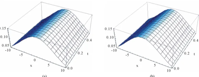
[image:4.595.59.537.432.707.2]
(a) (b)
Figure 4. (a) The exact solution for t = 0.5 and −10 ≤ x ≤ 10; (b) Numerical solution with new modification for t = 0.5 and −10 ≤ x ≤ 10.
ADM to solve the RLW equation. The decomposition series solutions are converge very rapidly in real physical problems. The numerical results we obtained justify the advantage of this methodology, even in the few terms approximation is accurate. The method is tested on the problem of single solitary motion and high accuracy was achieved with the L2 and L∞ error norms. The new
Laplace ADM presented here is for the RLW equation, but it can be implemented to a large number of physically important nonlinear wave problems.
REFERENCES
[1] D. H. Peregrine, “Calculation of the Development of an Undular Bore,” Journal of Fluid Mechanics, Vol. 25, No. 2, 1966, pp. 321-330. doi:10.1017/S0022112066001678 [2] Kh. O. Abdullove, H. Bogalubsky and V. G. Markhankov,
“One More Example of Inelastic Soliton Interaction,” Physics Letters A, Vol. 56, No. 6, 1976, pp. 427-428. [3] J. L. Bona, W. G. Pritchard and L. R. Scott, “Numerical
Schemes for a Model of Nonlinear Dispersive Waves,” Journal of Computer Physics, Vol. 60, 1985, pp. 167-196. [4] P. J. Jain and L. Iskandar, “Numerical Solutions of the
Regularized Long Wave Equation,” Computer Methods in Applied Mechanics and Engineering, Vol. 20, No. 2, 1979, pp. 195-201. doi:10.1016/0045-7825(79)90017-3 [5] L. R. T. Gardner, G. A. Gardner and A. Dogan, “A Least
Squares Finite Element Scheme for RLW Equation,” Communications in Numerical Methods in Engineering, Vol. 11, No. 1, 1995, pp. 59-68.
doi:10.1002/cnm.1640110109
[6] İ. Daǧ and M. N. Özer, “Approximation of the RLW Equation by the Least Square Cubic B-Spline Finite
Ele-ment Method,” Applied Mathematical Modelling, Vol. 25, No. 3, 2001, pp. 221-231.
doi:10.1016/S0307-904X(00)00030-5
[7] Y. keskin and G. Oturanc, “Numerical Solution of Regu-larized Long Wave Equation by Reduced Differential Transform Method,” Applied Mathematical Sciences, Vol. 4, No. 25, 2010, pp. 1221-1231.
[8] G. Adomian, “Nonlinear Stochastic Operator Equa-taions,” Academic Press, San Diego, 1986.
[9] G. Adomian, “Solving Frontier Problem of Physics: The Decomposition Method,” Kluwer Academic Publishers, Boston, 1994.
[10] E. Yusufoglu and A. Bekir, “Application of the Varia-tional Iteration Method to the Regularized Long Wave Equation,” Computer & Mathematics with Applications, Vol. 25, 2003, pp. 321-330.
[11] G. Adomian, “Modified Adomian Polynomials,” Mathe-matical Computation, Vol. 76, No. 1, 1996, pp. 95-97.
doi:10.1016/0096-3003(95)00186-7
[12] A.-M. Wazwaz and S. M. El-Sayed, “A New Modifica-tion of the Adomian DecomposiModifica-tion Method for Linear and Nonlinear Operators,” Applied Mathematics and Computation, Vol. 122, No. 3, 2001, pp. 393-405.
doi:10.1016/S0096-3003(00)00060-6
[13] T. S. El-Danaf, M. A. Ramadan and F. E. I. AbdAlaal, “The Use of Adomian Decomposition Method for Solv-ing the Regularized Long-Wave Equation,” Chaos, Soli-tons & Fractals, Vol. 26, No. 3, 2005, pp. 747-757.
doi:10.1016/j.chaos.2005.02.012
[image:5.595.92.508.83.245.2]