Amirkabir University of Technology (Tehran Polytechnic)
Vol. 45, No. 2, Fall 2013, pp. 43- 56
Amirkabir International Journal of Science& Research (Electrical & Electronics Engineering)
AIJ-EEE) )
*Corresponding Author, Email: [email protected]
Vol. 45, No. 2, Fall 2013 43
Fast SFFS-Based Algorithm for Feature Selection in
Biomedical Datasets
F. Shirbani
1and H. Soltanian Zadeh
2*
1-MSc. Student, Control and Intelligent Processing Center of Excellence (CIPCE), Electrical and Computer Engineering Department, University of Tehran, Tehran, Iran
2-Professor, Department of Diagnostic Radiology, Henry Ford Hospital, Detroit, MI, USA
2- Professor, School of Cognitive Sciences (SCS), Institute for Research in Fundamental Sciences (IPM), Tehran, Iran
ABSTARCT
Biomedical datasets usually include a large number of features relative to the number of samples.
However, some data dimensions may be less relevant or even irrelevant to the output class. Selection of an
optimal subset of features is critical, not only to reduce the processing cost but also to improve the
classification results. To this end, this paper presents a hybrid method of filter and wrapper feature selection
that takes advantage of a modified method of sequential forward floating search (SFFS) algorithm. The
filtering approach evaluates the features for predicting the output and complementing the other features. The
candidate subset generated by the filtering approach is used by k-fold cross validation of support vector
machine (SVM) with user-defined classification margin as a wrapper. Applications of the proposed SFFS
method to five biomedical datasets illustrate its superiority in terms of classification accuracy and execution
time relative to the conventional SFFS method and another previously improved SFFS method.
KEYWORDS
1- INTRODUCTION
A major problem in medical data analysis is “curse of dimensionality” [1-3], particularly in datasets with relatively few instances in a high-dimensional feature space [4]. Reducing the number of features not only may improve the classification accuracy and enhance understanding of computational models but also reduces the cost of database storage and management [5-7]. Therefore, feature reduction has become one of the major fields in biomedical data mining [6].
From the classification point of view, the main goal of feature reduction is to find an optimal feature subset that improves the classification performance [8-9]. To this end, either of the two common approaches of feature extraction and feature selection may be used [10]. Feature extraction methods such as principal component analysis combine the features to generate a smaller feature subset. On the other hand, feature selection methods omit some of the features to generate a smaller feature subset. The first approach blurs the physical meaning of the original features but the second approach preserves their meanings [11].
In most high dimensional datasets such as medical databases, there are non-informative features that may decrease the classification accuracy. Considering the advantages of feature selection algorithms like eliminating the effect of irrelevant information due to irrelevant features and preserving physical meaning of features, feature selection methods are usually preferred [9, 11]. Based on the interaction between feature selection and classification modules, these methods are categorized into three groups: (i) filter; (ii) wrapper; and (iii) hybrid [12-15].
Filter methods evaluate features by employing an independent test such as information entropy or statistical dependence but wrappers exploit specific machine learning algorithms to find an efficient subset [4, 16]. Each group has its own advantages and disadvantages. Filter-based techniques run fast but they do not benefit from a learning algorithm. Compared to the other methods, they lead to lower classification performance because no interaction is considered between classifier and features. On the other hand, wrappers often result in higher classification accuracy, but they are computationally expensive and thus inappropriate for large databases with many features. In addition, wrappers are less general than filters and must be re-run when switching from one learning algorithm to another [4, 7 and 16].
To benefit from the advantages of filter and wrapper methods, hybrid techniques have been developed. A typical hybrid approach uses both an independent test and
a performance evaluation function [5, 17]. Therefore, by limiting the search space of a wrapper and implementation of a learning algorithm in a filter, a hybrid method can be implemented that results in a classification with an excellent efficiency and performance. Different hybrid methods can be designed using various types of searching procedures, feature evaluation methods, and learning algorithms [4].
Many different filter approaches have been developed in recent years while much effort has been devoted to develop appropriate feature evaluation criteria. According to [18, 19], these criteria can be divided into 3 major groups: distance; information; and dependence. A distance measure finds the distance of class labels and attributes to generate feature importance scores. Relief algorithm is the most prominent method in this category [19]. An information measure computes the information gain of features as a measure for their selection. A well-known method that belongs to this category is C4.5. A dependence measure calculates the correlation between the features and class labels. The probability of error and average correlation coefficient methods are the well-known examples of this category [20].
Many efficient search algorithms have also been developed in recent years. A powerful and common approach is a genetic algorithm (GA) [21]. Importance score or sequential search and ARO are the other approaches [7, 22]. While several candidate solutions of feature subsets are maintained in GA, the sequential search methods determine the importance score of each feature and then search for the minimum number of features that maximize the classification accuracy [5, 7]. Researchers have studied these feature selection methods and shown that sequential methods result in better or at least comparable classification performance compared to GA [23-25].
Vol. 45, No. 2, Fall 2013 45
Thus, the new search algorithm is quicker and more accurate than the previous method. Finally, benefiting from an intelligent method of initial subset selection and a reliable wrapper method leads to the efficient results compared to the previous approaches.
The rest of the paper is organized as follows. Section 2 introduces filtering and wrapper feature selection methods. Section 3 presents a detailed explanation of the proposed feature selection algorithm that includes novel SFFS search method, search criteria, hybrid procedure, and a brief description of two other evaluation approaches. Section 4 describes the experimental results and compares the proposed method with two previous methods, using five biomedical datasets. Finally, Section 5 presents the concluding remarks.
2- FEATURE SELECTION 2-1- FILTER METHOD
The filter approach ranks features based on their characteristic and usually regardless of the classification accuracy. In this work, it selects candidate features based on their relevance [7]. Features are relevant if their values vary systematically with category membership, otherwise, they are irrelevant [26]. A redundant feature is also defined when it is correlated with other features. The above definitions lead to the following filter method of feature selection: A desired candidate subset includes features that are the most predictable of output while they have the least predictability of each other. In other words, a good feature subset contains features highly correlated with the class label, yet uncorrelated with each other [16]. To compute the output predictability of a feature, we apply the Relief algorithm. This instance based learning method ranks the features according to their relevance. The following description shows how the weights are updated in the Relief algorithm [18]:
In an iteration of the Relief algorithm, one data point is selected randomly. For each sample, the nearest miss instance (nearest data point from the opposite class) and the nearest hit instance (nearest data point from the same
class) are found [18, 27]. Distances between the data points are calculated using the Pythagorean distance definition. A feature weight is updated depending on how well its value distinguishes between similar instances of different classes [16, 27]. At the end, the features with higher relevancy weight are considered more predictable of the output.
Finally, predictability of a feature, P, is calculated by the ratio of an evaluation weight to the sum of all evaluation weights.
(2)
A good candidate feature should also be complementary to the features selected previously. In this study, the complementary property between a target feature and a subset of features is estimated by [4]:
(3)
Where pi is the Pearson correlation between a target feature (x) and a member of feature subset (yj). The value pi [-1, 1] indicates the correlation or dependency between 2 features and indicates their independency. The higher the value of for a target feature, the more complementary to the preselected feature.
The measure C, complementary of a feature and the subset Y, is calculated by averaging
independency of the target and any of the selected features in the subset:
(4)
Finally, the filter method criterion to find the efficient features is:
(5) Here, the two predictability and complementariness normalizing factors balance discrimination ability of a feature and its independence from the features selected previously. Consequently, M is computed for the features that are not selected previously and additional features are selected from those that have the highest M values.
2-2- WRAPPER METHOD
is computationally more expensive [27]. Several learning algorithms have been used in wrappers, and in most cases, classification accuracy has been used as a measure of feature selection. As a more reliable measure, we use the following average area under the ROC curve (AUC) of k-fold cross validation [4]:
(6)
As a learning algorithm, we apply SVM classification, which has shown great promise in high dimensional data classification such as biomedical datasets [28, 29]. A SVM classifier finds hyper-planes that produce largest separation between two data points in different classes. Regardless of kernel type, in the first step, SVM produces a decision value for each test data point. Then, it finds a proper threshold for classification. To calculate AUC for each data subset, we change the threshold from the smallest to the largest possible values and generate an ROC curve. Different non-linear kernels in the LIB_SVM MATLAB toolbox generate different decision values. By moving the margin, different points of the ROC curve are produced. Assume f(i), i=1, 2, …, m denote the vector of the decision values and “m” is the number of test data points. Then, the classification output is shown by y1(i) or y2(i), depending on the classifier that produces the greater AUC value.
(7)
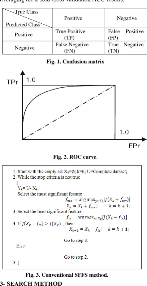
(8) Since we utilize binary class datasets in this research, the classifier outputs can be grouped in four possible categories. When a positive sample is classified correctly as positive, it is a true positive (TP) and when it is classified wrongly as negative, it is a false negative (FN). Similarly, when a negative sample is classified correctly as negative, it is a true negative (TN) and when it is classified wrongly as positive, it is a false positive (FP) (see Fig. 1). True positive rate (FPr) and false positive rate (FPr) that form two axes of an ROC curve are calculated by:
(9)
(10)
As shown in Fig. 2, a receiver operating characteristic (ROC) curve is created by changing threshold from the
minimum decision value to the maximum decision value which results in different TPr versus FPr. The AUC is calculated by integrating the area under the ROC curve. The average AUC for a set of features is calculated by averaging the k-fold cross validation AUC results.
Fig. 1. Confusion matrix
Fig. 2. ROC curve.
Fig. 3. Conventional SFFS method.
3- SEARCH METHOD
The proposed feature selection algorithm is a hybrid filter and wrapper method and applies an improved Sequential Forward Floating Search (SFFS) algorithm. Before explaining the proposed algorithm, SFFS is briefly explained.
3-1- SFFS METHOD
Sequential feature selection algorithms search for an efficient subset of features by aggregating the best features or eliminating the worst features iteratively [30]. This approach has progressed from one directional search of sequential forward selection (SFS) or sequential
True Class Predicted Class
Positive Negative
Positive True Positive
(TP)
False Positive (FP)
Negative False Negative
(FN)
Vol. 45, No. 2, Fall 2013 47
backward search (SBS) to the conventional methods of sequential forward floating search (SFFS) and sequential backward floating search (SBFS) that are bidirectional.
In one directional search methods, once a feature is selected in SFS (or eliminated in SBS), there is no way to discard (or add) this feature again. This is the main disadvantage of these methods. On the other hand, bidirectional search methods are able to reselect discarded features or delete selected ones, as they include both of the inclusion and exclusion parts. Fig. 3 shows the framework of the SFFS method.
SFFS starts the search from a null subset (or a random subset X0), performs an iterative procedure for selecting the most significant feature (fms) from the remaining dataset (Yk = U - Xk), adds it to Xk (Xk= Xk U fms) and then, repeatedly finds and deletes the least significant features (fls) from the new subset Xk. After each iteration, the results are compared to those of the previous step (Xk). If the outcome is improved, then (Xk+1 = Xk – fls) and this procedure continues repeatedly until reaching a specific criterion. The most and the least significant features are selected by applying a wrapper algorithm and an evaluation criterion.
3-2- PROPOSED ALGORITHM
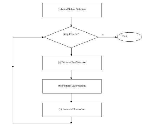
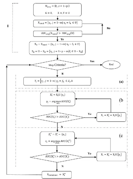
The proposed feature selection algorithm is a hybrid approach, which searches for an efficient subset of features by applying an improved SFFS method. The block diagram in Fig. 4 demonstrates the main steps of the proposed algorithm while the details are given in Fig. 5. As shown in Fig. 5, the method includes a main loop, preceded by selecting the first subset of features in part I. The main loop consists of three main steps: a) feature pre-selection using the proposed filter method; b) iterative procedure of aggregating the best features one by one until the wrapper measure stops increasing; and c) iterative procedure of removing the worst features one by one until the wrapper measure stops increasing.
Denoting Uqxp as the complete dataset where q and p indicate the number of data points and the number of features, the proposed algorithm in part I starts from a random subset of “m” features (X0) with the conditions explained below. Then, in the first step of the loop in part (a), the measure M in equation (5) is calculated for all the remaining features (p - m), and “n” features with relatively high evaluation values are pre-selected from Z0 = U - X0. The new pre-selected subset in each loop (i) is called Yi. In each iteration, Xi is assumed as selected feature subset and Yi as candidate feature subset.
In the second step of the loop in part (b), the SVM classification method is applied on Xi’, which is created by aggregating a candidate feature to Xi (Xi’ = Xi U
{yj}). The AUC is then calculated for each Xi’ and the candidate feature that increases AUCavg the most is selected as the best feature and added to the selected subset. This procedure repeats until no improvement is achieved. If adding no feature increases AUCavg, then Xi’ will be the same as Xi by the end of this part. The part (c) as the last step finds the worst feature of Xi and eliminates it from Xi’ (Xi’’= Xi’ - {xj}). The worst feature is discovered by the same wrapper measure used for identifying the best feature. Again, this procedure repeats until no improvement is achieved. These three steps repeat until the following steps result in the same subset of features.
The following conditions are important to the success of the proposed method.
The parameters “m” and “n” in parts I and (a) are properly selected based on the size of the dataset so that they do not lead to any hasty convergence or oscillatory and unstable results. If they are small compared to the total number of features, none of the candidate features may increase the wrapper measure and the algorithm may oscillate. On the other hand, if a relatively large number of features are pre-selected, the algorithm resembles the conventional SFFS method which is time consuming. Thus, we consider “m” to be about 20-25% and “n” to be 10-20% of the total number of features.
It is assumed that the first subset in part I is selected randomly. However, if it is selected completely at random, the execution cost may be high. To prevent this, m features are randomly selected and form the first selected subset if and only if the wrapper evaluation result of the selected subset exceeds the evaluation result of the whole dataset. Using this condition, the procedure terminates in a reasonable amount of time.
A K-fold cross-validation (K=5) of SVM is used to reduce chance relying results.
In pre-selection part (a), after calculating the measure “M”, instead of choosing “n” features with highest qualifications, relatively high values of the measure “M” are pre-selected. For example, n features are pre-selected randomly from one half or two thirds of the highest M values. This approach adds to the flexibility of the proposed algorithm since it increases the selection probability of a feature with a high value without selecting it for sure. Similarly, a feature with a low value is less probable to be selected but again not for sure. Figure 4: Proposed algorithm main steps
Fig. 4. Proposed algorithm main steps
TABLE 1. Experimented medical datasets used in this work
Name of dataset Number and type of features Number of data
points
Class label type/distribution
HBIDS (Human Brain Image
Database System) 29 continuous valued 160
2 Binary classes
(80 vs. 80) and (101 vs. 59)
WPBC (Wisconsin Prognostic
Breast Cancer) 32 continuous valued 198 1 Binary class (151 vs. 47)
WDBC (Wisconsin Diagnostic
Breast Cancer) 30 continuous valued 569 1 Binary class (357 vs. 212)
Arrhythmia heart data 206 continuous valued 430 1Binary class (245 vs. 185)
SPECTF (SPECTF heart data) 44 continuous valued 267 1 Binary class (212 vs. 55)
NNN
Stop Criteria?
(c) Features Elimination (b) Features Aggregation (a) Features Pre-Selection
Exit
Y
Vol. 45, No. 2, Fall 2013 49
Fig. 5. Proposed algorithm
4. EXPERIMENTAL RESULTS
The proposed feature selection algorithm is evaluated using five biomedical datasets with binary classes that contain two-label outcomes. Breast cancer Wisconsin Diagnostic (WDBC), breast cancer Wisconsin Prognostic (WPBC), the SPECTF heart data and Arrhythmia database available at UCI machine learning repository are four of the experimental datasets used in this research [31]. The first two datasets are complete, but the other two have the missing values. The incomplete features of WPBC are eliminated, while the missing values of Arrhythmia are replaced by applying the nearest neighbor method imputation. In addition, the miss-classified samples of Arrhythmia are excluded and the 15 output classes are depleted to two classes of normal and abnormal categories. The HBIDS dataset of Henry Ford Hospital collected from 160 temporal lobe epilepsy patients is the fifth dataset. It contains 108 numeric and nominal features. Excluding the nominal features and features with high percentage of missing values and applying mean imputation, missing value management leads in 29 numeric features. These features include information extracted from medical images, EEG analysis, and other disease-related information of the patients. The characteristics of the five datasets are summarized in Table 1. For a comparison study, two other methods of feature selection are applied to all datasets. The first method is the classical SFFS method, presented in Subsection3.1. The second one is a hybrid approach proposed by Peng and co-workers [4]. All methods in this paper were implemented and run by MATLAB 7.8 and a computer with properties as follows: Core 2Du with 2.26 GHz duration and 3 GB RAM.
This approach searches for efficient features by applying the conventional SFFS method. It uses a novel measure for pre-selection, which combines Pearson correlation for complementary ability and a simple threshold classifier for the predictability of a feature. In addition, it uses AUC of the SVM classifier as the wrapper method of feature evaluation. The efficient kernel and its parameters are found by optimizing a cross-validation based model selection criterion, applied to any of the complete datasets. In each iteration of SFFS, always, one feature (the one by which the wrapper measure becomes the highest) is added, even if AUC does not increase compared to the previous subset. Then, the worst features are eliminated one by one, if and only if the AUC measure increases by eliminations. After all, the results are compared by the previous subset results, and if there is no improvement, it starts again from the previous subset. Altogether, the feature aggregation always occurs at most one time in a loop, whereas
eliminations can happen from zero to several times. To apply the proposed feature selection method, we do the following.
1-
About m = 25% of the features are selected randomly with the condition of resulting greater AUC compared to the whole dataset.2-
In each iteration, about n = 15% of the remaining data is pre-selected with relatively high values of M. These features are selected randomly from 2/3 of the feature with the highest M values.3-
At the end of each loop, the selected features are compared with the previous loop. If the three following iterations generate the same features, the procedure stops.4-
In the beginning of the algorithm, about 10% of data samples are selected as an unseen evaluation dataset. However, the unbalance proportion of samples in two class labels is preserved so the evaluation data resembles a random sample of the complete dataset. The other 90% of the data samples contribute to the entire procedure. The evaluation results are reported on both evaluation dataset and the k-fold cross validation of the rest.5-
All wrapper evaluations are performed by the k-fold cross validation with k = 5.6-
To balance complementary and predictability coefficients, several w1 and w2 are examined such that w1 + w2 = 1. The ones that generate the highest accuracy are considered as the fixed coefficients for each of the datasets. These coefficients are found to be w1 = 0.6 , 0.7 and w2 = 0.4 , 0.3 for the data sets used in this work.7-
In each iteration of the k-fold cross validation with of the input dataset is used for training. Since 90% of the complete dataset is considered as the input dataset, the training data samples consist of of the complete dataset in any of the five cross validations.8-
The radial basis function (RBF) is applied as an efficient kernel for the WPBC dataset and polynomial functions are used for the other three datasets. Finding the efficient kernels and their optimized parameters depend on the specifications of the datasets.Vol. 45, No. 2, Fall 2013 51
TABLE 2. Results of applying the three methods on the five biomedical datasets:
(a) WDBC, (b) WPBC, (c) SPECTF (d) Arrhythmia and (e) HBIDS.
(a) WDBC
Mean AUC x100
Mean Accuracy %
Relative execution time
Standard deviation of AUC
Number of features selected
SFFS 99.2 98.3 325 0.06 11
Peng’s 99.7 98.9 185 0.05 16
Proposed 99.6 99.1 50 0.01 8
(b) WPBC
Mean AUC x100
Mean Accuracy %
Relative execution time
Standard deviation of AUC
Number of features selected
SFFS 72.9 86.6 256 0.50 19
Peng’s 76.3 88.2 60 0.10 10
Proposed 81.4 90.5 15 0.02 7
(c) SPECTF
Mean AUC x100
Mean Accuracy % Relative execution
time
Standard deviation of AUC
Number of features selected
SFFS 80.1 87.5 410 0.70 17
Peng’s 83.9 87.5 160 0.20 12
Proposed 86.5 92.7 23 0.03 9
(d) Arrhythmia
Mean AUC x100
Mean Accuracy % Relative execution
time
Standard deviation of AUC
Number of features selected
SFFS 66.4 68.7 1950 0.76 96
Peng’s 71.7 77.9 1242 0.52 63
Proposed 78.2 80.1 1038 0.11 49
(e) HBIDS
Mean AUC x100
Mean Accuracy %
Relative execution time
Standard deviation of AUC
Number of features selected
SFFS 78.6 84.3 623 0.90 13
Peng’s 82.5 86.6 131 0.01 10
Proposed 90.3 92.1 70 0.06 5
65 85 105
SFFS Peng's
method
suggested method
WDBC
WPBC
SPECTF
Arrhythmia
the reference [4] results. However, these differences are negligible and do not affect the comparison of two methods.
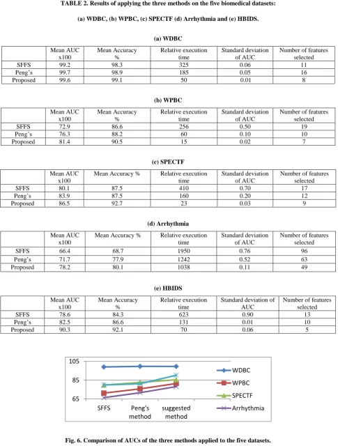
Table 2 illustrates that the proposed algorithm results in greater AUC and accuracy compared to the Peng’s method for all datasets except WDBC where the proposed algorithm is comparable to the Peng’s algorithm. These results illustrate that the proposed algorithm selects the most efficient features. The most recognizable achievement of the proposed algorithm is reduction of the execution time. To avoid presenting floating-point numbers for the execution times which represent for the whole process of 5 iterations, the actual execution times are multiplied by a constant (13.33 ms) and rounded to the nearest integer. This characteristic is very valuable especially in mining large-scale datasets. A comparison of the number of selected features in all cases confirms that this novel algorithm is able to pick a smaller number of features that generate a greater AUC. This is particularly useful for biomedical data mining that has relatively large number of features compared to the data samples.
Fig. 6 graphically compares the average AUC’s of three methods on five dataset.
5- DISCUSSION
Experimental results illustrate the efficiency of the proposed feature selection method in reducing the execution time and the number of features. They also show superiority of the proposed method to two related feature selection methods in their applications to five biomedical datasets. The other methods are SFFS, which is one of the best feature selection methods, and Peng’s algorithm, which is an enhanced version of SFFS. Advantages of the proposed method include an increased classification accuracy and AUC, decreased execution time, smaller AUC standard deviation, and more importantly, smaller sets of selected features in all cases. The only exception is AUC of WDBC where the proposed approach results in a slightly smaller yet comparable outcome. The combination of complementary and predictability measures in feature pre-selection is a source of improvement in algorithm efficiency as it also improves Peng’s method over conventional SFFS. The ability of a feature to complement a subset is retrieved by a measure derived from Pearson correlation in equation (3). Moreover, applying Relief algorithm as one of the best methods of filtering for feature selection produces an estimate of feature predictability. The efficiency of this method over simple threshold classifier leads to more efficient feature selections and shorter execution times. Since each dataset has its own characteristics, efficient contribution of the two measures may change from one case to another. To find optimal coefficients, we have conducted some experiments by varying [w1, w2] from
[1,0] to [0,1]. Fig. 7 shows the resulting accuracy and AUC values for all datasets. The first point in each diagram corresponds to the situation in which the M measure includes the complementary ability only. On the other hand, and the last point corresponds to the situation in which the predictability is considered only. Comparison of the classification results obtained by the proposed method and the Peng’s method in different combinations of the coefficients confirm the superiority of the proposed method to the Peng’s method.
The next innovation that makes this algorithm superior is in the features adding or removing technique. In each iteration of SFFS and the Peng’s method, the best feature among candidate features (in Peng’s) or among all features (in SFFS) is added to the final subset. Then, the worst features are found and eliminated one after another. The elimination process continues until reaching a specified condition such as no increase in accuracy or AUC. This means that in each iteration, one feature is certainly added to the subset even if the performance measure does not increase compared to the previous subset and the features elimination is done including this feature. After each iteration, the quality of the final result is compared with the previous step and if no improvement is attained, the new subset is discarded. Clearly, in this case, identification of the best and worst features may be useless and time consuming. In addition, in each iteration of both methods, at most one feature may be added. This procedure increases the execution time.
Vol. 45, No. 2, Fall 2013 53
Fi
g
.
7
.
Ac
cu
ra
cy
a
n
d
AU
C o
f
cl
a
ss
ifi
ca
tio
n
s re
sul
ts g
en
er
a
te
d
b
y
v
a
ry
in
g
w1
a
n
d
w2
c
o
efficie
n
ts f
o
r
th
e
fiv
e
d
a
ta
se
ts: (a
)
WDB
C; (b
)
WPBC;
(c
)
S
PECTF;
(d
)
Ar
rh
y
th
m
ia
;
a
n
d
(e
)
H
BID
There is another point that deserves a note here and that is the independency of the whole algorithm to the size and type of the datasets. Since no conditions or limitations are considered, this approach can be applied to large, non-biomedical datasets too. Nevertheless, testing of the proposed method on non-biomedical datasets was considered beyond the scope of this study.
Despite all the experiments reported above, the effectiveness of this algorithm could be theoretically predicted by comparing with other efficient similar optimization search methods such as ARO. In ARO algorithm, which is a model free optimization algorithm for real time applications, it is assumed that each solution in search space (feature subset in our method) is an organism in environment and only the most deserving ones can survive [22].
First of all, in ARO, an individual (parent) is randomly initiated (such as X0 in our method). Then it would reproduce an offspring ( ) and the parent and offspring would compete to survive based on their fitness function. If the offspring wins, it will replace its parent and be the new parent. Otherwise, the offspring is eliminated. In Our method as well, new subset of features is made by aggregating new features to the initial subset or deleting features from them. After producing any new subset, the parent ( ) and offspring ( ) compete in producing higher AUC of classification as a surviving measure. A few conditions for features pre-selection are considered in our algorithm to increase execution speed and avoid getting trapped in a local optimum feature subset just like ARO conditions which are set to guarantee the convergence.
Knowing that our proposed algorithm has similar searching structure to ARO, SFFS, and Peng’s algorithms, which are proved to be efficient, it is expected that this search algorithm is also efficient. Furthermore, the modifications made in our approach, including iterative aggregation /elimination of best/worst features in each iteration, would theoretically decrease the running time and increase the classification accuracy. The reason is that, on one hand, each iteration in our search method is not limited to the addition/exclusion of only one feature. Therefore, in a single search cycle, several changes may occur in the subset that would increase the execution speed of the algorithm. On the other hand, letting the least/most significant feature stay in/out of the selected subset may lead to further miss election and decrease the accuracy.
Altogether, from a theoretical point of view, as described above and by getting better practical results, this paper shows that the innovation and modifications
made in our proposed algorithm lead to impressive progress in the SFFS search algorithm in terms of execution time and accuracy [4, 10 and 22].
6- CONCLUSION
A new hybrid method of feature selection with a modified sequential search method is proposed for the classification of biomedical datasets. It includes a new filtering feature pre-selection measure. This measure benefits from combination of the Relief algorithm and the Pearson correlation as an evaluation of a feature’s predictability and complementarity. The proposed wrapper method is an optimized SVM method that selects the best or the worst features based on the average AUC measure of k-fold cross validation. Furthermore, the proposed search algorithm is a new modification of SFFS in which both of the feature aggregation and elimination tasks are repeated until no further improvement is achieved.
The results of our experiments on five biomedical datasets demonstrate the effectiveness of our proposed algorithm compared to the conventional SFFS algorithm and Peng’s method. The enhancements include an increase in the area under accuracy curve of data samples classification. In addition, the results show an explicit reduction in the relative execution time and the number of selected features. This is a valuable trait in mining large biomedical datasets as well as the other datasets with relatively large number of features.
ACKNOELEDGMENT
The work of the second author has been supported in part by NIH grant R01 EB013227.
REFERENCES
[1] J. Fan; J. Lv; “A selective overview of variable selection in high dimensional feature space”, Statistica Sinica, Vol. 20(1), pp. 101-148, 2010. [2] M. Pal; G. M. Foody; “Feature Selection for
Classification of Hyperspectral Data by SVM”, IEEE Trans. Geoscience and Remote Sensing, Vol. 48 , No. 5, pp. 2297-2307, 2010.
[3] Y. Liu; “Feature extraction and dimensionality reduction for mass spectrometry data”, Computers in Biology and Medicine, Vol. 39, pp. 818-823, 2009.
[4] Y. Peng; Z. Wu; J. Jiang; “A novel feature selection approach for biomedical data classification”, J. Biomedical Informatics, Vol. 43, pp. 15-23, 2010.
Vol. 45, No. 2, Fall 2013 55
library, Springer, Vol. 12, 2011.
[6] Y. Saeys; I. Inza; P. Larranaga; “A review of feature selection techniques in Bioinformatics”, Bioinformatics, Vol. 23, pp. 2507-2517, 2007. [7] Z. Aghbari; Bayesian Network,
<http://www.intechopen.com/books/bayesian- network/classification-of-categorical-and-numerical-data-on-selected-subset-of-features>, 2010.
[8] Y. Yang; X. Guan; J. You; “CLOPE: A fast and effective clustering algorithm for transactional data”, Proceeding of the eighth ACM SIGKDD International Conference on Knowledge Discovery and Data Mining, pp. 682–687, 2002. [9] H. Qin; X. Ma; T. Herawan; J. Mohamad Zain;
“MGR: An information theory based hierarchical divisive clustering algorithm for categorical data”, Knowledge-Based Systems, Vol. 67, pp. 401– 411, 2014.
[10] B. Pandey; R.B. Mishra; “Knowledge and intelligent computing system in medicine”, Computers in Biology and Medicine, Vol. 39, pp. 215-230, 2009.
[11] T. W. S Chow; P. Wang; E. W. M. Ma; “A new feature selection scheme using a data distribution factor for unsupervised nominal data”, IEEE Transactions on Systems, Man, and Cybernetics, Part B, Vol. 38, pp. 499-509, 2008.
[12] M. Blazadonakis; M. Zervakis; “Wrapper filtering criteria via linear neuron and kernel approaches”, Computers in Biology and Medicine, Vol. 38, pp. 894-912, 2008.
[13] R. Blanco; P. Larranaga; I. Inza; B. Sierra; “Gene selection for cancer classification using wrapper approaches”, International Journal of Pattern Recognition and Artificial Intelligence, Vol. 18, pp. 1373-1390, 2004.
[14] M. Pechenizkiy, A. Tsymbal; S. Puuronen; “Local dimensionality reduction and supervised learning within natural clusters for biomedical data analysis”, IEEE Transactions on Information Technology in Biomedicine, Vol. 10, pp. 533-539, 2006.
[15] X. Q. Zeng; G. Z. Li; J. Y. Yang; “Dimension reduction with redundant gene elimination for tumor classification”, BMC Bioinformatics, Vol. 9, S-6 2008.
[16] M. A. Hall; “Correlation-based feature selection for machine learning”, Ph.D. Thesis, Computer science department, University of Waikato at Hamilton, New Zealand, 1999.
[17] H. Liu; L. Yu; “Toward integrated feature selection algorithms for classification and clustering”, IEEE Transactions on Knowledge and Data Engineering, Vol. 17, pp. 491-502, 2005.
[18] K. Kira; L. A.Rendell; “The Feature Selection Problem: Traditional methods and a new algorithm”, Proceedings of Ninth National Conference on Artificial Intelligence, pp. 129-134, 1992.
[19] I. Kononenko; “Estimating attributes: Analysis and Extension of RELIEF”, Proceedings of European Conference on Machine Learning, pp. 171-182, 1994.
[20] V. Kariwala; L. Ye; Y. Cao; “Branch and bound method for regression-based controlled variable selection”, Computers & Chemical Engineering, Vol. 54, pp. 1–7, 2013.
[21] R.V. Rao; V.J. Savsani; D.P. Vakharia; “Teaching–Learning-Based Optimization: An optimization method for continuous non-linear large scale problems”, Information Sciences, Vol. 183, Issue 1, pp. 1–15, 2012.
[22] T. Mansouri; A. Farasat; M. B. Menhaj; M. Moghadam; “ARO: A new model free optimization algorithm for real time applications inspired by the asexual reproduction”, Expert Systems with Applications, Vol. 38, pp. 4866-4874, 2011.
[23] F. J. Ferri; P. Pudil; M. Hatef; J. Kittler; “Comparative study of techniques for large scale feature selection”, Machine Intelligence and Pattern Recognition, Vol. 16, pp. 403-413, 1994. [24] E. Yilmaz; “An expert system based on fisher
score and LS_SVM for cardiac Arrhythmia Diagnosis”, Computational and Mathematical Methods in Medicine, Vol. 2013, Article ID 849674, 6 pages, 2013.
[25] M. Kudo; J. Sklansky; “Comparison of algorithms that select features for pattern Recognition”, Pattern Recognition, Vol. 33, pp. 25-41, 2000. [26] E.Namsrai; T. Munkhdalai; “A feature
classification”, Journal of Information Processing Systems, Vol. 9, pp. 31-40, 2013.
[27] S. N. Ghazavi; T. W. Liao; “Medical data mining by fuzzy modeling with selected features”, Artificial Intelligence in Medicine, Vol. 43, pp. 195-206, 2008.
[28] Y. H. Peng; “A novel ensemble machine learning for robust microarray data Classification”, Computers in Biology and Medicine, Vol. 36, pp. 553-573, 2006.
[29] X. Zhang; X. Lu; “Recursive SVM feature selection and sample classification for mass-spectrometry and microarray data”, BMC Bioinformatics, Vol. 7, 2006.
[30] P. Somol; J. Novovicova J; P. Pudil; “Flexible-hybrid sequential floating search in statistical feature selection”, Lecture notes in computer science, Springer-Verlag, Vol. 41, pp. 632-639, 2006.
[31] A. Asuncion; D. J. Newman;