L. Chupin, A. M¨unch, Editors
GREEDY ALGORITHMS FOR HIGH-DIMENSIONAL NON-SYMMETRIC
LINEAR PROBLEMS
∗,∗∗E. Canc`
es
1, V. Ehrlacher
1and T. Leli`
evre
1Abstract. In this article, we present a family of numerical approaches to solve high-dimensional linear non-symmetric problems. The principle of these methods is to approximate a function which depends on a large number of variates by a sum of tensor product functions, each term of which is iteratively computed via a greedy algorithm [20]. There exists a good theoretical framework for these methods in the case of (linear and nonlinear) symmetric elliptic problems. However, the convergence results are not valid any more as soon as the problems under consideration are not symmetric. We present here a review of the main algorithms proposed in the literature to circumvent this difficulty, together with some new approaches. The theoretical convergence results and the practical implementation of these algorithms are discussed. Their behaviors are illustrated through some numerical examples.
R´esum´e. Dans cet article, nous pr´esentons une famille de m´ethodes num´eriques pour r´esoudre des probl`emes lin´eaires non sym´etriques en grande dimension. Le principe de ces approches est de repr´esenter une fonction d´ependant d’un grand nombre de variables sous la forme d’une somme de fonc-tions produit tensoriel, dont chaque terme est calcul´e it´erativement via un algorithme glouton [20]. Ces m´ethodes poss`edent de bonnes propri´et´es th´eoriques dans le cas de probl`emes elliptiques sym´etriques (lin´eaires ou non lin´eaires), mais celles-ci ne sont plus valables d`es lors que les probl`emes consid´er´es ne sont plus sym´etriques. Nous pr´esentons une revue des principaux algorithmes propos´es dans la litt´erature pour contourner cette difficult´e ainsi que de nouvelles approches que nous proposons. Les r´esultats de convergence th´eoriques et la mise en oeuvre pratique de ces algorithmes sont d´etaill´es et leur comportement est illustr´e au travers d’exemples num´eriques.
Introduction
High-dimensional problems arise in a wide range of fields such as quantum chemistry, molecular dynamics, uncertainty quantification, polymeric fluids, finance... In all these contexts, one wishes to approximate a function udepending ondvariatesx1, ...,xd whered∈N∗ is typically very large. Classically, the function uis defined
as the solution of a Partial Differential Equation (PDE) and cannot be obtained by standard approximation techniques such as Galerkin methods for instance. Indeed, let us consider a discretization basis withN degrees of freedom for each variate (N ∈N∗), so that the discretization space is given by
VN := Span
n
ψi(1)1 (x1)· · ·ψ(id)
d (xd), 1≤i1,· · · , id≤N
o
,
∗Funding from the Michelin company is acknowledged.
∗∗ Virginie Ehrlacher would like to thank Kathrin Smetana for very interesting discussions about symmetric formulations of
non-symmetric problems.
1Universit´e Paris Est, CERMICS, projet MICMAC, Ecole des Ponts Paristech - INRIA, 6 & 8 avenue Blaise Pascal, 77455
Marne-la-Vall´ee Cedex 2, France; e-mail: [email protected] & [email protected] & [email protected] c
EDP Sciences, SMAI 2013
where for all 1≤j≤d,ψi(j)
1≤i≤N is a family ofN functions which only depend on the variatexj. A Galerkin
method consists in representing the solutionuof the initial PDE as
u(x1,· · ·, xd)≈
X
1≤i1,···,id≤N
λi1,···,idψ (1)
i1 (x1)· · ·ψ (d)
id (xd),
and computing the set of Nd real numbers (λi1,···,id)1≤i1,···,id≤N. Thus, the size of the finite-dimensional problem to solve grows exponentially with the number of variates involved in the problem. Such methods cannot be implemented whendis too large: this is the so-calledcurse of dimensionality[2].
Several approaches have recently been proposed in order to circumvent this difficulty. Let us mention among others sparse grids [21], tensor formats [11], reduced bases [4] and adaptive polynomial approximations [6].
In this paper, we will focus on a particular set of methods, originally introduced by Ladev`ezeet al. to perform time-space variable separation [12], Chinesta et al. to solve high-dimensional Fokker-Planck equations in the context of kinetic models for polymers [1] and Nouy in the context of uncertainty quantification [15], under the name ofProgressive Generalized Decomposition (PGD) methods.
Let us assume that each variatexjbelongs to a subsetXj ofRmj, wheremj∈N∗ for all 1≤j≤d. For each
d-tuple (r(1),· · ·, r(d)) of functions such thatr(j)only depends onxj for all 1≤j≤d, we call atensor product function and denote byr(1)⊗ · · · ⊗r(d)the function which depends on all the variatesx1,· · ·, xdand is defined
by
r(1)⊗ · · · ⊗r(d):
X1× · · · × Xd → R
(x1,· · · , xd) 7→ r(1)(x1)· · ·r(d)(xd).
The approach of Ladev`eze, Chinesta, Nouy and coauthors consists in approximating the function u by a separate variable decomposition, i.e.
u(x1,· · · , xd)≈ n
X
k=1
r(1)k (x1)· · ·rk(d)(xd) = n
X
k=1
r(1)k ⊗ · · · ⊗r(kd)(x1,· · · , xd), (1)
for some n ∈ N∗. In the above sum, each term is a tensor product function. Each d-tuple of functions
r(1)k ,· · ·, r(kd) is iteratively computed in a greedy [20] way: once the firstk terms in the sum (1) have been computed, they are fixed, and the (k + 1)th term is obtained as the next best tensor product function to
approximate the solution. This will be made precise below.
Thus, the algorithm consists in solving several low-dimensional problems whose dimensions scale linearly with the number of variates and can be applied when classical methods are not. In this case, if we use a discretization basis withNdegrees of freedom per variate as above, the size of the discretized problems involved in the computation of a d-tuple rk(1),· · · , r(kd) is of the order ofN d and the total size of the discretization problems isnN d.
This numerical strategy has been extensively studied for the resolution of (linear or nonlinear) elliptic prob-lems [5, 10, 13, 18, 20]. More precisely, let ube defined as the unique solution of a minimization problem of the form
u= argmin
v∈V
E(v), (2)
where V is a reflexive Banach space of functions depending on thed variates x1, ..., xd, and E :V →R is a
coercive real-valued energy functional. Besides, for all 1≤j≤d, letVxj be a reflexive Banach space of functions
which only depend on the variate xj. The standard greedy algorithm reads:
(2) findr(1)n ,· · ·, r(nd)
∈Vx1× · · · ×Vxd such that
r(1)n ,· · · , r(nd)∈ argmin (r(1),···,r(d))∈Vx
1×···×Vxd
Eun−1+r(1)⊗ · · · ⊗r(d)
,
(3) setun=un−1+rn(1)⊗ · · · ⊗rn(d)andn=n+ 1.
Under some natural assumptions on the spacesV,Vx1, ...,Vxd and the energy functionalE, all the iterations of the greedy algorithm are well-defined and the sequence (un)n∈N∗ strongly converges inV towards the solution uof the original minimization problem (2).
This result holds in particular whenuis defined as the unique solution of
findu∈Vsuch that
∀v∈V, a(u, v) =l(v),
whereV is a Hilbert space,ais asymmetric continuous coercive bilinear form onV ×V andl is a continuous linear form on V. In this case, u is equivalently solution of a minimization problem of the form (2) with
E(v) = 1
2a(v, v)−l(v) for allv∈V.
However, there is no obvious generalization of the iterative algorithm presented above when the functionu is not defined as the solution of a minimization problem of the form (2). This situation typically occurs when uis defined as the solution of anon-symmetric linear problem
findu∈Vsuch that
∀v∈V, a(u, v) =l(v),
whereais a non-symmetric continuous bilinear form onV ×V andl is a continuous linear form onV. The aim of this article is to give an overview of the state of the art of the numerical methods based on the greedy iterative approach used in this non-symmetric linear context and of the remaining open questions concerning this issue. In Section 1, we present the standard greedy algorithm for the resolution of symmetric coercive high-dimensional problems and the theoretical convergence results proved in this setting. Section 2 explains why a naive transposition of this algorithm for non-symmetric problems is doomed to failure and motivates the need for more subtle approaches. Section 3 describes the provably converging algorithms existing in the literature for non-symmetric problems. All of them consist in symmetrizing the original non-symmetric problem by minimizing the residual of the equation in a well-chosen norm. However, depending on the choice of the norm, either the conditioning of the discretized problems may behave badly or several intermediate problems may have to be solved online, which leads to a significant increase of simulation times and memory needs compared to the original algorithm in a symmetric linear coercive case. So far, there are no methods avoiding these two problems and for which there are theoretical convergence results in the general case. In Section 4, we present some existing algorithms designed by Nouy [16] and Lozinski [14] to circumvent these difficulties and the partial theoretical results which are known for these algorithms. Section 5 is concerned with another algorithm we propose, for which some partial convergence results are proved. In Section 6, the behaviors of the different algorithms presented here are illustrated on simple toy numerical examples. Lastly, we present in the Appendix some possible tracks to design other methods, but for which further work is needed.
1.
The symmetric coercive case
1.1.
Notation
Let us first introduce some notation. Letdbe a positive integer,m1, ...,md positive integers andX1, ...,Xd
Letµx1, ...,µxd denote measures onX1, ..., Xd respectively. Let L 2(X1;µ
x1), ...,L 2(X
d;µxd) be associated
L2 spaces, i.e. vectorial spaces which are complete when endowed with the scalar products
∀f, g∈L2(Xj;µxj), hf, giXj :=
Z
Xj
f(xj)g(xj)µxj(dxj), ∀1≤j≤d,
and their associated normsk · kX1, ...,k · kXd. For instance, in the case whenX1= (0,1) andµx1 is the standard Lebesgue measure onX1, the spacesL2(0,1),Lper2 (0,1) andL20(0,1) :=
n
f ∈L2(0,1), R01f = 0oare examples of suchL2 spaces.
In the rest of this article, for the sake of simplicity, we will omit the reference to the measuresµx1, ...,µxd
and denote byL2(X1) =L2(X1;µ
x1), ...,L 2(X
d) =L2(Xd;µxd).
We introduce the space L2(X
1× · · · × Xd) := L2(X1)⊗ · · · ⊗L2(Xd). This space is a Hilbert space when
endowed with the natural scalar product
∀f, g∈L2(X1× · · · × Xd), hf, gi:=
Z
X1×···×Xd
f(x1,· · ·, xd)g(x1,· · ·, xd)µx1(dx1)· · ·µxd(dxd),
and the associated norm is denoted byk · kX1×···×Xd.
Let V ⊂L2(X
1× · · · × Xd), Vx1 ⊂L
2(X1), ...,V
xd ⊂L
2(X
d) be Hilbert spaces endowed respectively with
scalar products denoted byh·,·iV,h·,·iVx1, ...,h·,·iVxd and associated normsk · kV,k · kVx1, ...,k · kVxd.
We defineV′, V′
x1, ...,Vxd′ as the dual spaces ofV,Vx1, ...,Vxd with respect to theL
2 scalar productsh·,·i,
h·,·iX1, ...,h·,·iXd. These dual spaces are endowed with their natural normsk · kV′ etc.
Lastly, the Riesz operatorRV :V →V′ is defined by
∀v, w∈V, hv, wiV =hRVv, wiV′,V. It holds in particular that kvkV =kRVvkV′. Similar operators RVx
1, ..., RVxd are introduced for the spaces
Vx1, ...,Vxd.
For anyd-tuple r(1),· · · , r(d)∈Vx1× · · · ×Vxd, we define the tensor product functionr
(1)⊗ · · · ⊗r(d) as follows
r(1)⊗ · · · ⊗r(d):
X1× · · · × Xd → R
(x1,· · · , xd) 7→ r(1)(x1)· · ·r(d)(xd).
In the particular case whend= 2, we shall denote respectivelyx1,X1,m1,Vx1 byx,X,mx,Vxandx2,X2, m2,Vx2 byt,T, mt,Vt.
Besides, for any Banach spacesH1,H2, the space of bounded linear operators fromH1toH2will be denoted byL(H1, H2).
1.2.
Theoretical results
We recall here the theoretical framework of the standard greedy algorithm in the coercive symmetric case.
Let us consider the problem
findu∈V such that
∀v∈V, a(u, v) =l(v), (3) where
• a(·,·) is asymmetric, coercivecontinuous bilinear form onV ×V;
Then, problem (3) is equivalent to the minimization problem
u= argmin
v∈V E(
v), (4)
where
∀v∈V, E(v) :=1
2a(v, v)−l(v). (5)
The greedy algorithm reads: (1) letu0= 0 andn= 1; (2) definer(1)n ,· · ·, r(nd)
∈Vx1× · · · ×Vxd such that
r(1)n ,· · · , r(nd)∈ argmin (r(1),···,r(d))∈V
x1×···×Vxd
Eun−1+r(1)⊗ · · · ⊗r(d)
; (6)
(3) defineun=un−1+rn(1)⊗ · · · ⊗r(nd) and setn=n+ 1.
Let us denote by
Σ :=nr(1)⊗ · · · ⊗r(d), r(1)∈Vx1,· · · , r (d)∈V
xd
o
(7)
and make the following assumptions:
(A1) Span(Σ)V =V;
(A2) Σ is weakly closed in V.
These assumptions are usually satisfied in the case of classical Sobolev spaces [5].
Theorem 1.1. Assume that (A1) and (A2) are satisfied. Then, for alln∈N∗, there exists at least one solution
r(1)n ,· · ·, r(nd)
∈Vx1× · · · ×Vxd (not necessarily unique) to (6) and any solution satisfiesr (1)
n ⊗ · · · ⊗r(nd)6= 0 if and only if un−16=u. Besides, the sequence (un)n∈N∗ strongly converges towards uinV.
The following Lemma will be used later. Although the proof is given in [10], we recall it here for the sake of self-containedness.
Lemma 1.1. For all v∈V, let us denote bykvka:=
p
a(v, v). Then, for alln∈N∗,
rn(1)⊗ · · · ⊗r(nd)
a=(r(1),···,r(d))∈Vx sup
1×···×Vxd, r(1)⊗···⊗r(d)6=0
a u−un−1, r(1)⊗ · · · ⊗r(d)
r(1)⊗ · · · ⊗r(d)
a
. (8)
Proof. Let us prove (8) for n = 1. The proof is similar for larger n ∈ N∗. The d-tuple r(1)1 ,· · ·, r1(d) ∈
Vx1× · · · ×Vxd solution of (6) forn= 1 equivalently satisfies:
r(1)1 ,· · ·, r(1d)∈ argmin (r(1),···,r(d))∈Vx
1×···×Vxd
1 2
u−r(1)⊗ · · · ⊗r(d)2
a. (9)
The Euler equations associated to this minimization problem read: for all δr(1),· · ·, δr(d)∈Vx1× · · · ×Vxd,
which implies that
r(1)1 ⊗ · · · ⊗r1(d)
2
a =a
u, r(1)1 ⊗ · · · ⊗r(1d). (10) Let now r(1),· · ·, r(d)∈Vx1× · · · ×Vxd be such thatr
(1)⊗ · · · ⊗r(d)6= 0. Using (9) and (10), it holds that
u− a
u, r1(1)⊗ · · · ⊗r (d) 1
r(1)1 ⊗ · · · ⊗r (d) 1 2 a
r(1)1 ⊗ · · · ⊗r(1d)
2 a =
u−r(1)1 ⊗ · · · ⊗r(1d)
2 a≤ u−
a u, r(1)⊗ · · · ⊗r(d)
r(1)⊗ · · · ⊗r(d)2
a
r(1)⊗ · · · ⊗r(d)
2 a . Therefore,
au, r1(1)⊗ · · · ⊗r1(d)2
r1(1)⊗ · · · ⊗r1(d)2
a
≥a u, r
(1)⊗ · · · ⊗r(d)2
r(1)⊗ · · · ⊗r(d)2
a
.
Taking the supremum over all r(1),· · · , r(d)∈Vx1×· · ·×Vxdsuch thatr
(1)⊗· · ·⊗r(d)6= 0 yields the result. Equation (8) implies in particular that for alln∈N∗,
rn(1)⊗ · · · ⊗ · · ·rn(d)
a =(r(1),···,r(d)sup)∈Vx
1×···×Vxd
l r(1)⊗ · · · ⊗r(d)−a u
n−1, r(1)⊗ · · · ⊗r(d)
r(1)⊗ · · · ⊗r(d)
a
. (11)
Let us rewrite the greedy algorithm in the particular case whend= 2. (1) Letu0= 0 and n= 1;
(2) define (rn, sn)∈Vx×Vtsuch that
(rn, sn)∈ argmin
(r,s)∈Vx×Vt
E(un−1+r⊗s) ; (12)
(3) defineun=un−1+rn⊗sn and set n=n+ 1.
For the sake of simplicity, in the rest of the article, all the algorithms will be presented in the case whend= 2. The generalization of the approaches to a larger number of variatesdis straightforward unless mentioned.
The Euler equations associated to the minimization problem (12) read
a(un−1+rn⊗sn, δr⊗sn+rn⊗δs) =l(δr⊗sn+rn⊗δs), ∀(δr, δs)∈Vx×Vt. (13)
As a consequence of Theorem 1.1, provided that the set
Σ ={r⊗s, r∈Vx, s∈Vt} (14)
satisfies assumptions (A1) and (A2), at the first iteration of the algorithm (n = 1), as soon as the forml is nonzero, there exists at least one solution (r1, s1)∈Vx×Vtof
a(r1⊗s1, δr⊗s1+r1⊗δs) =l(δr⊗s1+r1⊗δs), ∀(δr, δs)∈Vx×Vt,
such thatr1⊗s16= 0.
In practice, at each iteration n∈N∗, a pair (rn, sn)∈Vx×Vt is computed via the resolution of the Euler
• choose rn(0), s(0)n
∈Vx×Vtand setm= 1; • findr(nm), s(nm)
∈Vx×Vtsuch that
aun−1+r(nm)⊗s(nm−1), δr⊗s(nm−1)
=lδr⊗s(nm−1)
, ∀δr∈Vx,
aun−1+r(nm)⊗s(nm), r(nm)⊗δs
=lr(nm)⊗δs
, ∀δs∈Vt;
(15)
• setm=m+ 1.
This fixed-point algorithm is numerically observed to converge exponentially fast in most situations, although, at least to our knowledge, there is no rigorous proof in the general case.
2.
The non-symmetric case
2.1.
General framework
Let us now consider the case of a non-symmetric linear problem of the form
findu∈V such that
∀v∈V, a(u, v) =l(v), (16)
where
• a(·,·) is anonsymmmetriccontinuous bilinear form onV ×V;
• l is a continuous linear form onV. In the rest of the article, we will assume that
(A3) problem (16) has a unique solutionu∈V for any continuous linear forml∈L(V,R).
We denote byA ∈L(V, V) the operator defined by
∀v, w∈V, hAv, wiV =a(v, w),
and byLthe element ofV such that
∀v∈V, hL, viV =l(v).
We also introduce the operator A:V →V′ and the linear formL∈V′ defined byA=RVAandL=RVL
so that the unique solutionuto (16) is also the unique solution to the problem
findu∈V such that Au=LinV′.
It follows from assumption (A3) thatAandA are invertible operators.
2.2.
Prototypical examples
Let us present two prototypical examples we will refer to throughout the rest of the paper.
• The first one is
findu∈H1
0(X)⊗L2(T) such that
−∆xu+bx· ∇xu+u=f in D′(X × T), (17)
withf ∈H−1(X)⊗L2(T) andb
x∈Rmx. For this problem,V =H01(X)⊗L2(T),V′ =H−1(X)⊗L2(T) and
∀u, v∈V, a(u, v) =RX ×T (∇xu· ∇xv+v(bx· ∇xu) +uv), ∀v∈V, l(v) =RThf, viH−1(X),H1
• The second example is
findu∈H01(X × T) such that
−∆x,tu+b· ∇x,tu+u=f inD′(X × T), (18)
withf ∈H−1(X ×T) andb= (bx, bt)∈Rmx×Rmt. For this problem,V =H01(X ×T),V′ =H−1(X,T) and
∀u, v∈V, a(u, v) =RX ×T (∇x,tu· ∇x,tv+v(b· ∇x,tu) +uv), ∀v∈V, l(v) =hf, viH−1(X ×T),H1
0(X ×T). In this case,A=−∆x,t+b· ∇x,t+ 1.
2.3.
Failure of the standard greedy algorithm
Problem (16) cannot be written as a minimization problem of the form (4) with an energy functional given by (5). The definition of the greedy algorithm via the minimization problems (6) or (12) cannot therefore be transposed to this case. However, a natural way to define the iterations of a greedy algorithm for the non-symmetric problem (16) is to define iteratively for n ∈ N∗ the pair (rn, sn) ∈ Vx×Vt as a solution of the
following equation
a(un−1+rn⊗sn, δr⊗sn+rn⊗δs) =l(δr⊗sn+rn⊗δs), ∀(δr, δs)∈Vx×Vt, (19)
by analogy with the Euler equations (13). This is the so-calledPGD-Galerkin algorithm [3].
Actually, there are cases whenl6= 0 and any solution (r1, s1)∈Vx×Vtof the first iteration of the algorithm
a(r1⊗s1, δr⊗s1+r1⊗δs) =l(δr⊗s1+r1⊗δs), ∀(δr, δs)∈Vx×Vt, (20)
necessarily satisfiesr1⊗s1= 0. Such an algorithm cannot converge since the approximationun = n
X
k=1 rk⊗sk
given by the algorithm is equal to 0 for anyn∈N∗. Besides, this situation may occur even when the norm of
the antisymmetric part of the bilinear forma(·,·) is arbitrarily small. Let us give an explicit example.
Example 2.1. Let X =T = (−1,1) andµx (respectively µt) be the Lebesgue measure on X (respectively on T). Let b∈R,Vx=H1
per(−1,1),Vt=L2(−1,1) andV =Vx⊗Vt. Consider the non-symmetric problem (16) with
∀v, w∈V, a(v, w) =
Z
X ×T
(∇xv· ∇xw+ (b· ∇xv)w+vw), and
∀v∈V, l(v) =
Z
X ×T
f v,
with f ∈L2
per(−1,1)⊗L2(−1,1). Problem (16) is equivalent to
find u∈Hper1 (−1,1)⊗L2(−1,1) such that
−∆xu+b∇xu+u=f in D′(R× T). (21) In this context, equations (20) read
find (r1, s1)∈Hper1 (−1,1)×L2(−1,1)such that
hR1
−1|s1(t)|
2dti(−r′′
1(x) +br1′(x) +r1(x)) =
R1
−1f(x, t)s1(t)dt,
hR1
−1 |r1′(x)|2+|r1(x)|2
dxis1(t) =R−11f(x, t)r1(x)dx,
since the periodic boundary conditions on r1 imply that R−11r1(x)r′1(x)dx= 0.
Unlike the symmetric case, there exists an infinite set of functionsf ∈L2per(−1,1)⊗L2(−1,1)such thatf 6= 0 and any solution(r1, s1)∈Vx×Vt of equations (22) necessarily satisfies r1⊗s1 = 0for any arbitrarily small value of|b|. This is the case for example whenf(x, t) =φ(x−t)for all(x, t)∈R×(−1,1)withφ∈L2
per(−1,1) an odd real-valued function.
Let us argue by contradiction. If (r1, s1)∈Vx×Vt is a solution to (22) such thatr1⊗s16= 0, up to some rescaling, we can assume that
Z 1
−1
|s1(t)|2dt=
Z 1
−1
|r1′(x)|2+|r1(x)|2
dx=λ >0.
Thus, we can rewrite (22) as
−r1′′(x) +br1′(x) +r1(x) = 1 λ
Z 1
−1
f(x, t)s1(t)dt,
s1(t) = 1 λ
Z 1
−1
f(x, t)r1(x)dx.
Plugging the second equation into the first one, we obtain
−r′′1(x) +br1′(x) +r1(x) = 1 λ2 Z 1 −1 Z 1 −1
f(x, t)f(y, t)dt
r1(y)dy. (23)
Let us denote by g(x, y) =R−11f(x, t)f(y, t)dt for all (x, y)∈R2. As φ is an odd,2-periodic function, it holds that
g(x, y) =
Z 1
−1
f(x, t)f(y, t)dt
=
Z 1
−1
φ(x−t)φ(y−t)dt
= −
Z 1
−1
φ(x−t)φ(t−y)dt
= −
Z 1+y
−1+y
φ(x−y−u)φ(u)du
= −
Z 1
−1
φ(x−y−u)φ(u)du.
Taking the Fourier transform of equation (23) yields that for allk∈πZ,
(|k|2+ibk+ 1)br1(k) =− 4
λ2
b
φ(k) 2
b
r1(k),
where
b
r1(k) =1 2
Z 1
−1
PRACTICE
THEORY
Dual norm residual minimization
PGD−Galerkin
Minimax
Dual Greedy
X−Greedy
Decomposition residual minimization
OK
Additional regularity on the right−hand side is needed though.
The conditioning of the resulting problems scale quadratically with the conditioning
of the original problem.
Need to solve several small− or high− dimensional
symmetric coercive problems
converge towards the true solution.
OK in finite dimension provided that the
compared to its implicit part. explicit part of the bilinear form is small enough
OK but slow
Diverges if the explicit part of the bilinear form is too large.
in practice.
Not clear how to implement the algorithm Same situation as the Dual−Greedy
OK OK OK OK
OK for separated operators
OK in finite dimension when
Problems in infinite dimension There are cases where the algorithm does not L2
V =Vx⊗Vt
Figure 1. Summary of the different greedy algorithms used for non-symmetric high-dimensional linear problems.
Futhermore, λ ∈ R∗+ and φb(0) = 0 (φ is an odd function). Thus, since φb(k) is a purely imaginary number,
−φb(k)2=bφ(k)2and a solutionr1necessarily satisfiesbr1(k) = 0for allk∈πZ, which yields a contradiction.
This example clearly shows that a naive transposition of the greedy algorithm to the non-symmetric case by analogy with the Euler equations (13) obtained in the symmetric case may be doomed to failure.
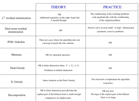
This article presents a review of some methods which aim at circumventing this difficulty. A particular highlight is set on the practical implementation of these methods and on the existence of theoretical rigorous convergence results. The properties of the different algorithms which are dealt with in this article are summarized in Figure 1. In particular, the algorithms which are markedOK in thePracticecolumn are those which
• do not suffer from conditioning problems;
• no extra loop of the greedy algorithm are needed to implement the method in practice.
3.
Residual minimization algorithms
idea is to symmetrize (16) using a reformulation as a residual minimization problem in a well-chosen norm. These algorithms are also calledMinimum Residual PGDin the literature [3].
3.1.
Minimization of the residual in the
L
2(
X × T
)
norm
Let us assume thatL∈L2(X × T) and that there existsD(A)⊂V a dense subdomain ofL2(X × T) such thatA(D(A))⊂L2(X × T). The mappingA:D(A)→L2(X × T) defines a linear operator onL2(X × T). Let us assume moreover that (A, D(A)) is a closed operator. This implies in particular thatD(A), endowed with the scalar product
∀v, w∈D(A), hv, wiD(A)=hv, wi+hAv, Awi, is a Hilbert space.
A first approach, inspired by [9], consists in applying a standard greedy algorithm on the energy functional
E(v) =kAv−Lk2L2(X ×T), ∀v∈D(A).
Let us consider the case when
A=
p
X
i=1
A(xi)⊗A(ti)
where for all 1≤i≤p,A(xi) andAt(i)are operators onL2(X) andL2(T) with domainsD
A(xi)
andDA(ti)
respectively. We denote byDx=Tpi=1D
A(xi)
andDt=Tpi=1D
A(ti), and assume thatDxandDtare dense
subspaces of L2(X) andL2(T) respectively and are Hilbert spaces, when endowed with the scalar products
∀v, w∈Dx, hv, wiDx =hv, wiX+ p
X
i=1
D
A(xi)v, A(xi)wE
X,
and
∀v, w∈Dt, hv, wiDt =hv, wiT +
p
X
i=1
D
A(ti)v, A
(i)
t w
E
T .
The greedy algorithm reads: (1) letu0= 0 and setn= 1;
(2) define (rn, sn)∈Dx×Dt such that
(rn, sn)∈ argmin
(r,s)∈Dx×Dt
kA(un−1+r⊗s)−Lk2L2(X ×T); (24)
(3) setun=un−1+rn⊗sn andn=n+ 1.
Let us denote by ΣD:={r⊗s, r∈D
x, s∈Dt}. From Theorem 1.1, provided that
(B1) SpanΣDD(A)=D(A);
(B2) ΣD is weakly closed inD(A);
the sequence (un)n∈N∗ strongly converges towardsuin D(A).
In the case of problem (17),A=Ax⊗AtwithAx=−∆x+b·∇x+1 andAt= 1,D(A) = H2(X)∩H01(X)
⊗
L2(T),D
x=D(Ax) =H2(X)∩H01(X) andDt=D(At) =L2(T).
For problem (18), A= A(1)x ⊗A(1)t +A
(2)
x ⊗A(2)t with A
(1)
x =−∆x+bx· ∇x+ 1, A(1)t = 1, A
(2)
x = 1 and
Actually, when L is regular enough, i.e. if L ∈ D(A∗), where A∗ denotes the adjoint of A and D(A∗) its
domain, this method is equivalent to performing a standard greedy algorithm on the symmetric coercive problem
A∗Au=A∗L.
The Euler equations associated to the minimization problems (24) read
hA(un−1+rn⊗sn)−L, A(δr⊗sn+rn⊗δs)i= 0, ∀(δr, δs)∈Dx×Dt.
This method suffers from several drawbacks though. Firstly, the right-hand side L needs more regularity than necessary for problem (16) to be well-posed (we needL∈L2(X × T) instead ofL∈V′).
Secondly, and more importantly, the conditioning of the associated discretized problems behaves badly since it scales quadratically with the conditioning of the original problem Au=L.
3.2.
Minimization of the residual in the dual norm
In order to avoid the conditioning problems encountered when minimizing the residual in the L2(X × T) norm, another method consists in performing a greedy algorithm on the energy functional
E(v) =kAv−Lk2V′ =kR−1
V (Av−L)k
2
V, ∀v∈V.
Here, the residual Av−L is evaluated in the dual norm k · kV′. In this method, the right-hand side L does not need to be more regular than L∈ V′ and this approach is equivalent to performing the standard greedy algorithm on the symmetric coercive problem
A∗(RV)−1Au=A∗(RV)−1L.
The conditioning of the resulting problem scales linearly with the conditioning of the originalAu=Lproblem. The algorithm reads:
(1) letu0= 0 andn= 1;
(2) let (rn, sn)∈Vx×Vt such that
(rn, sn)∈ argmin
(r,s)∈Vx×Vt
k(RV)−1[A(un−1+r⊗s)−L]k2V; (25)
(3) setun=un−1+rn⊗sn andn=n+ 1.
Provided that Σ defined by (14) satisfies assumptions (A1) and (A2), we infer from Theorem 1.1 that the sequence (un)n∈Nstrongly converges touinV.
The Euler equations associated with the minimization problems (25) read: for all (δr, δs)∈Vx×Vt,
R−V1[A(un−1+rn⊗sn)−L], R−V1[A(δr⊗sn+rn⊗δs)]V = 0,
or equivalently,
A(un−1+rn⊗sn)−L, RV−1[A(δr⊗sn+rn⊗δs)]
V′,V = 0.
However, even if the conditioning problem of the previous method is avoided, this algorithm still requires the inversion of the operatorRV.
In the case whenV =Vx⊗Vt, the dual spaceV′satisfiesV′=Vx′⊗Vt′, so that the operatorRV =RVx⊗RVt
is a tensorized operator and R−V1 = R−Vx1⊗R−Vt1. A prototypical example of this situation is given by the problem (17), where we have V′
R−V1 = (−∆x)−1⊗1 and carrying out the above greedy algorithm requires the computation of several
low-dimensional Poisson problems, which remains doable but increases the time and memory needs compared to a standard greedy algorithm in the symmetric coervive case whereb=bx= 0.
The situation is even more intricate when V 6=Vx⊗Vt, since the operatorRV is not a tensorized operator
in general. A prototypical example of this situation is problem (18) where V′ = H−1(X × T), R
V =−∆x,t
and R−V1 cannot be expanded as a finite sum of tensorized operators. These intermediate symmetric coercive high-dimensional can be solved with a standard greedy algorithm presented in Section 1, but this considerably increases the time needed to run a simulation.
In this particular case, sinceRV =−∆x⊗1−1⊗∆tis the sum of two tensorized operators which commute
with one another, we can use an approach described in [11]. This method consists in using an approximate expansion of the inverse of the Laplacian operator, constructed as follows. The functionh:x∈[x0,+∞)7→ x1 (wherex0is a positive real number) can be approximated by a sum of exponential functions of the form
1 x≈
N
X
l=1
Cle−clx,
for some N ∈ N∗ and where (Cl)1≤l≤N and (cl)1≤l≤N a two sets of well-chosen real numbers, depending on
x0. Provided that x0 satisfies x0 <min(1, λx1, λt1), where λx1 (respectively λt1) is the lowest eigenvalue of the operator −∆x onH01(X) with respect to the L2(X) scalar product (respectively the lowest eigenvalue of the operator −∆t on H01(T) with respect to the L2(T) scalar product), since both the operators −∆x⊗1 and −1⊗∆tcommute, R−V1can be approximated by
R−V1 ≈ PNl=1Cle−cl(−∆x⊗1−1⊗∆t)
= PNl=1Cle−cl∆x⊗e−cl∆t.
(26)
The computation of the expansion (26) only involves the computation of the exponential of small-dimensional operators. But of course, to have a reliable approximation of this operator, the numberN of terms in the above approximation may be very large. Besides, an explicit expansion is not always available for a general operator R−V1.
The algorithms presented in the following sections are attempts to find numerical methods which
• avoid the conditioning problem inherent to the method described in Section 3.1;
• avoid the use of inverse operators such asR−V1in the approach using the dual norm.
Of course, a natural idea would be to find a suitable norm to minimize the residual to avoid the conditioning and inversion problems. So far, no norms with such properties have been proposed.
In Section 4, we present algorithms already existing in the literature, namely those suggested by Anthony Nouy [16] and Alexe¨ı Lozinski [14]. In Section 5, a new algorithm is proposed. The known partial convergence results for these methods are presented and some details on the numerical implementations of these algorithms are provided.
4.
Algorithms based on dual formulations
In this section, we present some classes of algorithms based on dual formulations of the non-symmetric problem (16).
4.1.
MiniMax algorithm
A first algorithm based on a dual formulation of problem (16) is theMiniMax algorithmproposed by Nouy [16]. The algorithm reads as follows:
(2) let (rn,ern, sn,sen)∈Vx2×Vt2such that
(rn,ern, sn,esn)∈arg max
(r,ees)∈Vx×Vt(r,s)min∈Vx×VtJn(r⊗s,er⊗es), (27)
where for allv,ve∈V,
Jn(v,ev) =
1 2kvk
2
V −a(un−1+v,ev) +l(ev); (3) setun=un−1+rn⊗sn andn=n+ 1.
At each iterationn∈N∗, the computation of a quadruplet (rn,ern, sn,esn)∈Vx2×Vt2 satisfying (27) is done
by solving the stationarity equations
a(un−1+rn⊗sn,ern⊗δse+δer⊗sen) =l(ern⊗δes+δer⊗esn), ∀(δer, δes)∈Vx×Vt,
a(rn⊗δs+δr⊗sn,ern⊗esn) =hrn⊗δs+δr⊗sn, rn⊗sniV, ∀(δr, δs)∈Vx×Vt. (28)
In practice, for each n ∈ N∗, these equations are solved through a fixed-point procedure where the pairs
(rn,ren)∈Vx2 and (sn,esn)∈Vt2 are computed iteratively. More precisely, the fixed-point algorithm reads: • setm= 0, and choose an initial guessrn(0),ren(0), s(0)n ,es(0)n
∈Vx2×Vt2; • findr(nm+1),ern(m+1)
∈V2
x such that
aun−1+rn(m+1)⊗sn(m), δre⊗es(nm)
=lδer⊗es(nm)
, ∀δer∈Vx,
aδr⊗s(nm),ren(m+1)⊗es(nm)
=Dδr⊗s(nm), rn(m+1)⊗s(nm)
E
V , ∀δr∈Vx; • finds(nm+1),se(nm+1)
∈V2
t such that
aun−1+rn(m+1)⊗sn(m+1),re(nm+1)⊗δes
=ler(nm+1)⊗δes
, ∀δes∈Vt,
arn(m+1)⊗δs,ren(m+1)⊗es(nm+1)
=Drn(m+1)⊗δs, rn(m+1)⊗s(nm+1)
E
V , ∀δs∈Vt; • setm=m+ 1.
In [17], it is proved that in the case when a =ax⊗at where ax is a continuous bilinear form on Vx×Vx
and at a continuous bilinear form onVt×Vtand V =Vx⊗Vt, the algorithm converges. However, there is no
convergence result in the full general case.
4.2.
Greedy algorithms for Banach spaces
Another family of dual greedy algorithms is inspired from the methods suggested by Temlyakov in [20] for Banach spaces and was proposed by Lozinski [14] in order to deal with the resolution of high-dimensional problems of the form (16).
4.2.1. Greedy algorithms for general Banach spaces
For the sake of simplicity, let us present two particular greedy algorithms proposed by Temlyakov in the context of Banach spaces, namely theX-Greedyand theDual Greedy algorithms.
Let (X,k · kX) be a reflexive Banach space and D a dictionary of X, i.e. a subset of X such that for all
g∈ D,kgkX= 1 and Span(D) X
Letf ∈X. The aim of both the Dual Greedy and the X-Greedy algorithms is to give an approximation of f as a linear combination of vectors of the dictionaryD. These numerical methods are generalizations of the Pure Greedyalgorithm, which is defined for Hilbert spaces. WhenX is a Hilbert space endowed with the scalar producth·,·iX, the Pure Greedy algorithm can be interpreted in two equivalent ways, namely:
Pure Greedy algorithm (1):
(1) letf0= 0,r0=f andn= 1;
(2) letgn∈ Dandαn∈Rsuch that (assuming existence)
krn−1−αngnkX= min
g∈D, α∈Rkrn−1−αgkX; (3) letfn=fn−1+αngn,rn=rn−1−αngn andn=n+ 1;
and
Pure Greedy algorithm (2):
(1) letf0= 0,r0=f andn= 1;
(2) letgn∈ Dsuch that (assuming existence)
hrn−1, gniX = max
g∈Dhrn−1, giX;
(3) letαn ∈Rsuch that
krn−1−αngnkX= min
α∈Rkrn−1−αgnkX; (4) letfn=fn−1+αngn,rn=rn−1−αngn andn=n+ 1.
WhenX is a Hilbert space, the two versions of the Pure Greedy algorithm are equivalent, but this is not the case anymore as soon asX is a general Banach space.
TheX-Greedyalgorithm corresponds to the extension of the first version of the Pure Greedy algorithm: (1) letf0= 0,r0=f andn= 1;
(2) letgn∈ Dandαn∈Rsuch that (assuming existence)
krn−1−αngnkX= min
g∈D, α∈Rkrn−1−αgkX; (29) (3) letfn=fn−1+αngn,rn=rn−1−αngn andn=n+ 1.
TheDual Greedyalgorithm generalizes the second version of the Pure Greedy algorithm and is slightly more subtle. It is based on the notion ofpeak functional. For any non-zero elementf ∈X, we say thatFf ∈X′ is a
peak functional forf ifkFfkX∗ = 1 andFf(f) =kfkX. TheDual Greedy algorithm reads: (1) letf0= 0,r0=f andn= 1;
(2) letFrn−1∈X∗ be a peak functional forrn−1and letgn ∈ Dsuch that (assuming existence)
gn ∈argmax g∈D
Frn−1(g); (30)
(3) letαn ∈Rsuch that
αn∈argmin α∈R
krn−1−αgnkX; (31)
Slightly modified versions (relaxed versions) of the X-Greedy and Dual Greedy algorithms are proved to converge in [20] provided that the spaceX and the dictionaryDsatisfy some additional assumptions, detailed below. Actually, in these relaxed algorithms, (29), (30) and (31) are respectively replaced by
krn−1−αngnkX≤µn min
g∈D, α∈Rkrn−1−αgkX; (32) Frn−1(gn)≥νnmax
g∈DFrn−1(g); (33)
krn−1−αngnkX≤κnmin
α∈Rkrn−1−αgnkX; (34) where (µn)n∈N, (νn)n∈Nand (κn)n∈Nare well-chosen sequences of real numbers such that for alln∈N∗,µn ≥1,
νn≤1 andκn≥1.
We define the modulus of smoothness of the Banach spaceX by
∀β∈R, ρ(β) := sup
kxkX=kykX=1
1
2(kx+βykX+kx−βykX)−1
.
The Banach space (X,k · kX) is said to be uniformly smooth [20] if
lim
β→0 ρ(β)
β = 0.
Let us point out that if a Banach space (X,k · kX) is uniformly smooth, then the mappingG:x∈X 7→ kxkX
is Fr´echet-differentiable.
The relaxed versions of the X-Greedy and Dual Greedy algorithms are proved to converge [20] provided that
(B1) Span(D)k·kX =X;
(B2) RDis weakly closed inX;
(B3) X is a uniformly smooth Banach space.
We do not write here these relaxed versions of the algorithms for the sake of brevity and refer to [20].
4.2.2. Special Banach spaces for non-symmetric high-dimensional problems
Let us now present how these ideas were adapted by Lozinski to the case of high-dimensional non-symmetric problems. We begin here with the description of the particular Banach spaces involved. Let us assume in the rest of Section 4.2 that the operatorA−1:V →V is bounded.
A Banach space with good theoretical properties but which cannot be used in practice
The spaceV is now endowed with the following dual norm
∀v∈V, kvkA= sup
w∈V, w6=0 a(v, w)
kwkV
=kAvkV =kAvkV′.
Actually, since the linear operator Ais bounded onV, the space (V,k · kA) is a reflexive Banach space whose
dual space is (V,k · k(A∗)−1) where
∀v∈V, kvk(A∗)−1 = sup
w∈V, w6=0 a(w, v)
kwkV
=k(A∗)−1vk
Let us show that the Banach space (V,k · kA) and the dictionary
D={r⊗s, r∈Vx, s∈Vt, kr⊗skA= 1}
satisfy assumptions (B1), (B2) and (B3).
Let us begin with the proof of (B1) and (B2). Since the set of tensor product functions
Σ ={r⊗s, r∈Vx, s∈Vt}=RD
is assumed to be weakly closed in (V,k · kV) and to satisfy Span(Σ)
(V,k·kV)
=V (assumptions (A1) and (A2)), (B1) and (B2) are direct consequences of the fact thatAandA−1belong to the spaceL(V, V) (i.e. are bounded operators). For instance,L((V,k · kV),R) =L((V,k · kA),R) since
∀l∈L((V,k · kV),R), 1 kAkL(V,V)
klkL((V,k·kV),R)≤ klkL((V,k·kA),R)≤ kA
−1k
L(V,V)klkL((V,k·kV),R).
Let us now prove (B3). Since the operatorA is invertible, the modulus ρA of smoothness of (V,k · kA) is equal to the modulus of smoothnessρof (V,k · kV). Indeed, for allβ ∈R,
ρA(β) = sup
v,w∈V,kvkA=kwkA=1
1
2(kv+βwkA+kv−βwkA)−1
= sup
v,w∈V,kAvkV=kAwkV=1
1
2(kAv+βAwkV +kAv−βAwkV)−1
= sup
v,w∈V,kvkV=kwkV=1
1
2(kv+βwkV +kv−βwkV)−1
=ρ(β).
Since (V,k · kV) is a Hilbert space,
ρA(β)
β =
ρ(β) β β−→→00, and (V,k · kA) is a uniformly smooth Banach space.
To implement the X-Greedy or Dual Greedy algorithms in practice in this context, one needs to compute the normk · kA (see (29) and (31)). Since for allv∈V,kvkA=kAvkV =kR−V1AvkV, this requires the resolution
of several intermediate low- or high-dimensional problems to compute the inverse of the operatorRV. Actually,
this approach is equivalent to the one described in Section 3.2 and the same practical issues have to be faced in this context.
Another more practical Banach space
The idea of Lozinski is to replace this norm by a weaker one, easier to compute,
∀v∈V, kvkiA= sup
(r,s)∈Vx×Vt, r⊗s6=0
a(v, r⊗s)
kr⊗skV
Actually, denoting byk · ki theinjective normonV [8], defined by
∀v∈V, kvki = sup
(r,s)∈Vx×Vt, r⊗s6=0
hv, r⊗siV kr⊗skV
,
it holds that for allv ∈V,kvkiA=kAvki. Reasoning as above, the Banach space (V,k · kiA) has exactly the
same properties as (V,k · ki).
Since Σ is weakly closed inV, and since for allv∈V,kvki ≤ kvkV, Σ is also weakly closed in (V,k · ki). But,
in the full general case, the Banach space (V,k · ki) and hence the Banach space (V,k · kiA) are not uniformly
smooth. Actually, these spaces may not even be reflexive. Indeed, let us assume thatV =Vx⊗Vtand thatk·kV
is the associated cross-norm, in other words that for all (r, s)∈Vx×Vt,kr⊗skV =krkVxkskVt. It holds that [8]
(V,k · ki) is isomorphous toK(Vx, Vt), the Banach space of compact operators fromVx toVt endowed with the
operator norm. Since K(Vx, Vt) is not a reflexive space (K(Vx, Vt)∗ =S1(Vx, Vt) andS1(Vx, Vt)∗ =L(Vx, Vt)
where S1(Vx, Vt) denotes the set of trace-class operators fromVxto Vt), there is no guarantee of convergence
of the relaxed versions of the X-Greedy or Dual Greedy algorithms presented above.
The finite-dimensional cross-norm case
However, in the case when Vx and Vt are finite-dimensional and V = Vx⊗Vt, the spaces K(Vx, Vt) and
L(Vx, Vt) are identical. The space (V,k · ki) is then reflexive and uniformly smooth. Indeed, ifVx=Rmx and
Vt = Rmt, since k · kVx and k · kVt both derive from the scalar products h·,·iVx and h·,·iVt, there exist two
invertible matricesP ∈Rmx×mx and Q∈Rmt×mt such that ∀r∈Rmx, krkVx=kP rkF
mx, ∀s∈Rmt, kskVt =kQskF
mt,
where k · kFmx and k · kFmt denote respectively the Frobenius norms on R
mx and Rmt. Thus, (V,k · k i) is
isometrically isomorphic toRmx×mt seen asK(Vx, Vt), endowed with the norm
∀M ∈Rmx×mt, kMki= sup r∈Rmx, r6=0
kQM rkFmt kP rkFmx
=kQM P−1k2,
where
∀M ∈Rmx×mt, kMk2= sup r∈Rmx, r6=0
kM rkFmt krkFmx
.
Actually, (Rmx×mt,k · k2) is a uniformly smooth Banach space [19]. Thus, greedy algorithms for Banach spaces do converge in this setting.
4.2.3. Practical implementation of the algorithms
X-Greedy algorithm
The X-Greedy algorithm reads: (1) letu0= 0 andn= 1;
(2) find (rn, sn)∈Vx×Vtsuch that
(rn, sn)∈ argmin
(r,s)∈Vx×Vt
(3) setun=un−1+rn⊗sn andn=n+ 1.
From the definition of the normk · kiA (see (35)), the second step of the algorithm can be rewritten as
(2) find (rn, sn)∈Vx×Vtsuch that
(rn, sn) ∈ argmin(r,s)∈Vx×Vtsup(er,es)∈Vx×Vt
l(er⊗es)−a(un−1+r⊗s,er⊗es)
ker⊗eskV
= argmin(r,s)∈Vx×Vtsup(er,es)∈Vx×Vt,ker⊗eskV=1l(re⊗es)−a(un−1+r⊗s,er⊗se).
(37)
From a practical point of view, at each iterationn∈N∗, the functions (rn,ren, sn,esn)∈V2
x×Vt2are obtained
by solving the stationarity equations associated with (37), namely by solving the following coupled problem
find (rn,ren, sn,esn)∈Vx2×Vt2 such that for all (δr, δr, δs, δe es)∈Vx2×Vt2,
hern⊗esn,ern⊗δes+δer⊗esniV +a(un−1+rn⊗sn,ern⊗δes+δre⊗esn) =l(ern⊗δes+δer⊗sen),
a(rn⊗δs+δr⊗sn,ern⊗esn) = 0.
The X-Greedy algorithm has not been implemented in practice yet. Indeed, it is not clear how to compute a solution of the above stationarity equations since using a fixed-point algorithm procedure similar to the one presented in Section 4.1 for the MiniMax algorithm would always lead toren⊗esn = 0, due to the form of the
second equation.
Dual Greedy algorithm
Let us describe here how Lozinski adapted the Dual Greedy algorithm for the resolution of high-dimensional non-symmetric linear problems.
A remaining issue concerns the construction of a peak functional Frn−1 for the residual rn−1 = u−un−1 which is used in the second step of the algorithm (30). Actually, the true peak functional is not computed but only an approximation of this functional by an optimal tensor product function in a sense which is made precise below.
The adapted Dual Greedy algorithm reads: (1) setu0= 0 andn= 1;
(2) (computation of an approximate peak functional for the residualrn−1=u−un−1with a tensor product function) find (ern,esn)∈Vx×Vtsuch that
(ern,esn)∈ argmax
(r,ees)∈Vx×Vt,kre⊗eskV=1
a(u−un−1,er⊗es) = argmax (er,se)∈Vx×Vt,ker⊗eskV=1
l(er⊗es)−a(un−1,er⊗se); (38)
(3) (Step 2 of the Dual Greedy algorithm, see (30)) find (rn, sn)∈Vx×Vtsuch that
(rn, sn)∈ argmax
(r,s)∈Vx×Vt,kr⊗skiA=1
a(r⊗s,ern⊗esn); (39)
(4) (Step 3 of the Dual Greedy algorithm, see (31)) findαn∈Rsuch that
αn∈argmin α∈R
ku−un−1−αrn⊗snkiA= argmin
α∈R
sup
(er,es)∈Vx×Vt,ker⊗eskV=1
l(re⊗es)−a(un−1+αrn⊗sn,er⊗es); (40)
(5) setun=un−1+αnrn⊗sn andn=n+ 1.
The Euler-Lagrange equations associated with the minimization problem (38) read: for all (δer, δes)∈Vx×Vt,
for someλn∈Rsatisfyingλnkren⊗senk2V =λn=l(ern⊗esn)−a(un−1,ren⊗esn).
The Euler-Lagrange equations associated to the minimization problem (39) can be rewritten as follows: (rn, sn)∈Vx×Vtis solution of
a(rn⊗δs+δr⊗sn,ren⊗esn) =µna(rn⊗δs+δr⊗sn,brn⊗bsn), ∀(δr, δs)∈Vx×Vt,
where (brn,bsn)∈Vx×Vtis such that
(brn,bsn)∈ argmax
(br,bs)∈Vx×Vt,kbr⊗bskV=1
a(rn⊗sn,br⊗bs), (41)
andµn =a(rn⊗sn,ern⊗esn). Besides, if the pair (brn,bsn) satisfies (41), it holds that
a(rn⊗sn,brn⊗δsb+δbr⊗bsn) =νnhrbn⊗bsn,rbn⊗δbs+δbr⊗bsniV, ∀(δbr, δbs)∈Vx×Vt,
with νn =a(rn⊗sn,rbn⊗sbn) =krn⊗snkiA = 1. This yields to a coupled problem on (rn, sn) and (rbn,bsn).
Lozinski the noticed that, if (rn, sn) is solution to (39), (brn,sbn) = (ern,esn) is solution of (41) in the sense that
(ern,esn)∈ argmax
(br,bs)∈Vx×Vt,kbr⊗bskV=1
a(rn⊗sn,br⊗bs).
The Euler-Lagrange equations can be rewritten as
a(rn⊗sn,ern⊗δes+δer⊗esn) =hern⊗esn,ern⊗δes+δre⊗esniV, ∀(δr, δe es)∈Vx×Vt,
by takingµn=a(rn⊗sn,ern⊗esn) =krn⊗snkiA= 1.
The Euler equations associated with (40) read
a(u−un−1−αnrn⊗sn,ren⊗esn) = 0,
yielding toαn=a(u−un−1,ren⊗sen) =λn.
Finally, replacingαnrn⊗sn byrn⊗sn, the iterations of the Dual Greedy algorithm are computed in practice
as follows:
(1) letu0= 0 andn= 1;
(2) find (rn,ren, sn,esn)∈Vx2×Vt2 such that for all (δr, δr, δs, δe se)∈Vx2×Vt2,
hern⊗esn,ern⊗δse+δer⊗esniV =l(ern⊗δse+δer⊗sen)−a(un−1,ern⊗δes+δer⊗esn),
a(rn⊗sn,ern⊗δes+δer⊗esn) =l(ern⊗δes+δre⊗esn)−a(un−1,ren⊗δes+δre⊗esn);
(3) setun=un−1+rn⊗sn andn=n+ 1.
These equations lead to two decoupled problems on (rn, sn) and (ern,sen). Each of them is solved through a
fixed-point procedure similar to (15) described in details in Section 6.3.1. Some numerical tests are presented in Section 6, which illustrate the convergence of this algorithm.
5.
The Decomposition algorithm
Let us now present a new algorithm based on a decomposition of the bilinear form a. The bilinear form a can always be written as
a(·,·) =bs(·,·) +b(·,·) (42)
wherebs(·,·) is a symmetric coercive continuous bilinear form onV×V andb(·,·) a (not necessarily symmetric)
continuous bilinear form onV ×V. In the sequel,bs(·,·) (respectivelyb(·,·)) will be referred to as theimplicit
Example 5.1. Let us introduce as (respectively aas) the symmetric part (respectively antisymmetric part) of
a(·,·), defined by:
∀v, w∈V, as(v, w) =
1
2(a(v, w) +a(w, v)), (43)
and
∀v, w∈V, aas(v, w) =
1
2(a(v, w)−a(w, v)). (44)
Provided thatas is coercive, the decompositiona(·,·) =as(·,·) +aas(·,·)is admissible in the sense of (42).
Let us denote byBsandBthe bounded operators onV defined by
∀v, w∈V, bs(v, w) =hBsv, wiV, ∀v, w∈V, b(v, w) =hBv, wiV.
Sincebsis coercive, the operatorBsis invertible.
The principle of the algorithm we consider in this section to solve problem (16) consists in expliciting the part b of the bilinear form as a right-hand side source term. More precisely, one can consider the following fixed-point algorithm:
(1) choose a starting guessu0∈V and set n= 1; (2) letun be the unique solution to
∀v∈V, bs(un, v) =l(v)−b(un−1, v); (45)
(3) setn=n+ 1.
In other words, un =F(un−1) where for all v∈V,F(v) =Bs−1(L − Bv). If kBs−1BkL(V,V)<1, the mapping F : V → V is a contraction and it follows from the Picard fixed-point theorem that the sequence (un)n∈N strongly converges inV towards the solutionuof the initial problem (16).
A natural approach thus consists in solving problem (45) at each iteration n∈N∗ using a standard greedy
procedure. Provided that the greedy expansion obtained at each iteration n ∈ N∗ is accurate enough, the
sequence (un)n∈Ngiven by this algorithm strongly converges inV towardsu.
However, the principle of this method requires to compute a full greedy loop at each iteration n∈ N∗. In
order to save computational time, we now introduce the following algorithm, in which only one tensor product function is computed at each iterationn∈N∗.
Decomposition algorithm:
(1) letu0= 0 andn= 1;
(2) find (rn, sn)∈Vx×Vtsuch that
(rn, sn)∈ argmin
(r,s)∈Vx×Vt
1
2bs(un−1+r⊗s, un−1+r⊗s)−l(r⊗s)−b(un−1, r⊗s); (46)
(3) setun=un−1+rn⊗sn and setn=n+ 1.
The bilinear form b(·,·) is explicited as a right-hand side, whereas bs(·,·) remains implicit. This justifies the
terminology introduced in the beginning of the section.
Equation (46) can be rewritten equivalently as
(rn, sn) ∈ argmin(r,s)∈Vx×Vt
1
This means that for each n ∈ N∗, rn⊗sn is a tensor product solution to the first iteration of the greedy
algorithm applied to the following symmetric coercive problem
findu∈V such that
∀v∈V, bs(u, v) =l(v)−bs(un−1, v)−b(un−1, v) =l(v)−a(un−1, v).
As explained above, such an algorithm is expected to converge only if the normkB−1
s BkL(V,V)is small enough. Actually, in the case when the spacesVxandVtare finite dimensional, the following result holds:
Proposition 5.1. If Vx andVt are finite dimensional, there existsκ >0 such that if
kBs−1BkL(V,V)≤κ, (47)
then the sequence (un)n∈N∗ defined by the Decomposition algorithm strongly converges touin V.
Proof. Since Vt and Vx are assumed to be finite dimensional, from assumption (A1), so is V. Let κ := kB−1
s BkL(V,V). Let us denote by h·,·iVe = bs(·,·) the scalar product on V induced by the symmetric
bilin-ear formbs, and byk · kVe the associated norm.
LetL ∈e V and B ∈e L(V, V) be defined by
∀v∈V, l(v) =hLe, viVe,
∀v, w∈V, b(v, w) =hBev, wiVe.
Actually, Be = B−1
s B and Le = Bs−1L. This implies that for all v ∈ V, kAevkVe ≤ κkvkVe. Besides, I +Be=
B−1
s (Bs+B) =Bs−1A, whereI denotes the identity operator onV.
The proof relies on the fact that all norms are equivalent in finite dimension. In particular, let us define the injective norm k · keι by
∀v∈V, kvkeι= sup
(r,s)∈Vx×Vt
hv, r⊗siVe
kr⊗skVe .
Then, there existsα >0 such that
∀v∈V, kvkVe ≤αkvkeι.
Besides, for allv∈V,kvkeι≤ kvkVe.
Let us introduce Uen:=L −e Beun−un =Bs−1(L − Aun). For alln∈N∗,Uen is the vector ofV such that
∀v∈V, hUen, viVe =l(v)−a(un, v).
Forn≥1, the Euler equations associated to (46) read:
bs(un−1+rn⊗sn, rn⊗δs+δr⊗sn) =l(rn⊗δs+δr⊗sn)−b(un−1, rn⊗δs+δr⊗sn), ∀(δr, δs)∈Vx×Vt.
As a consequence,l(rn⊗sn)−a(un−1, rn⊗sn)−bs(rn⊗sn) =hUen−1−rn⊗sn, rn⊗sniVe = 0, which implies
that kUen−1kV2e =kUen−1−rn⊗snk2Ve +krn⊗snk2Ve. Furthermore, from Lemma 1.1, we have
krn⊗snkVe = sup
(r,s)∈Vx×Vt, r⊗s6=0
hUen−1, r⊗siVe
It holds that
kUen−1k2Ve − kUenkV2e = kUen−1kV2e− kUen−1−rn⊗sn−Bern⊗snk2Ve
= kUen−1kV2e− kUen−1−rn⊗snk2Ve− kBern⊗snk2Ve
+2hBern⊗sn,Uen−1−rn⊗sniVe
= krn⊗snk2Ve− kBern⊗snk2Ve−2hBern⊗sn,Uen−1−rn⊗sniVe
≥ (1−κ2)krn⊗snk2Ve −2κkrn⊗snkVekUen−1−rn⊗snkVe
≥ (1−κ2)krn⊗snk2Ve −2κkrn⊗snkVekUen−1kVe
≥ (1−κ2)krn⊗snk2Ve −2καkrn⊗snkVekUen−1keι
= (1−κ2−2ακ)krn⊗snk2Ve
= (1−κ2−2ακ)kUen−1k2eι.
If κ is small enough to ensure that 1−κ2 −2ακ > 0, the sequence (kUenkVe)n∈N∗ is non-increasing, hence
convergent. Thus, the series of general terms (kUen−1k2Ve − kUenk2Ve)n∈N∗ and (kUenk2
e
ι)n∈N∗ are convergent. This yields
kUenkeι −→ n→∞0,
and, as all norms are equivalent in finite dimension,
kUenkVen−→→∞0.
Ifκ <1, the operator (I+Be)−1 is continuous fromV toV for the normk · k
e
V, and ku−unkVe =kA−
1L−u
nkVe =
Bs−1A
−1
B−s1L −un
e
V =k(I+Be)
−1(L−e (I+Be)u
n)kVe =k(I+Be)−
1Ue
nkVen−→→∞0.
Since the normk · kVe is equivalent to the normk · kV, we obtain the desired result.
Unfortunately, the rateκin (47) strongly depends on the dimensions ofVxandVt, as shown in the proof of
Proposition 5.1. However, in some simple numerical experiments we performed with this algorithm, the rateκ does not seem to depend on the dimension, as illustrated in Section 6. The analysis of this numerical observation is work in progress.
A possible way to obtain a decomposition such as (42) satisfying (47) is to consider preconditioners for the initial antisymmetric problem. Problem (16) can be rewritten as
findu∈V such that
u= (I − CA)u+CL, (48)
whereCis a well-chosen continuous linear operator onV such thatkI − CAkL(V,V)is as small as possible. With this formulation, one can consider the following algorithm:
(1) letu0= 0 andn= 1;
(2) find (rn, sn)∈Vx×Vtsuch that
(rn, sn)∈ argmin
(r,s)∈Vx×Vt
1
(3) setun=un−1+rn⊗sn andn=n+ 1.
The bilinear form associated with the continuous operator CAneeds to be easy to compute on tensor product functions. At least in the case when V is finite dimensional, ifkI − CAkL(V,V) is small enough, the sequence
(un)n∈N∗ converges strongly inV towards the solutionuof (16). However, finding a suitable operatorCis not an easy task in general.
6.
Numerical results
6.1.
Presentation of the toy problems
In this section, we present the two toy problems we consider in these numerical tests. Let bx, bt ∈ R,
mx=mt= 1 and X =T = (−1,1).
The first toy problem is inspired from Example 2.1. In the continuous setting, we define
• V :=L2
per((−1,1), Hper1 ((−1,1),C)) =L2per((−1,1),C)⊗Hper1 ((−1,1),C);
• Vx:=Hper1 ((−1,1),C);
• Vt:=L2per((−1,1),C);
• f ∈L2
per((−1,1)2,C);
• for allu, v∈V,
a(u, v) :=
Z 1
−1
Z 1
−1
∇xu· ∇xv+ (bx· ∇xu)v+uv,
and
l(v) :=
Z 1
−1
Z 1
−1 f v.
The second toy problem is the following
• V :=H1
per((−1,1)2,C));
• Vx:=Hper1 ((−1,1),C);
• Vt:=Hper1 ((−1,1),C);
• f ∈L2
per((−1,1)2,C);
• for allu, v∈V,
a(u, v) :=
Z 1
−1
Z 1
−1
∇xu· ∇xv+∇tu· ∇tv
+
Z 1
−1
Z 1
−1
((bx· ∇xu+bt· ∇tu)v+uv),
and
l(v) :=
Z 1
−1
Z 1
−1 f v.
It can be easily checked in the two cases that the Hilbert spacesV,VxandVtsatisfy assumptions (A1) and
(A2). Besides, the sesquilinear forma:V ×V →Cis continuous and satisfies assumption (A3). Our aim is to
approximate the functionu∈V such that
∀v∈V, a(u, v) =l(v). (50)
We introduce finite-dimensional discretization spaces defined as follows. For all k ∈ Z, let ex
k : X ∋x 7→
1
√
2e
ikx andet
k:T ∋t7→ √12eikt. ForNx, Nt∈N∗, we define
VtNt := Spanetk, −Nt≤k≤Nt ,
andVNx,Nt :=VxNx⊗VtNt.
We then consider the Galerkin approximation of problem (50) in the discretization spaceVNx,Nt, i.e. find u∈VNx,Nt such that
∀v∈VNx,Nt, a(u, v) =l(v). (51) Forusolution of (51), we denote byU = (ukl)|k|≤Nx,|l|≤Nt ∈C(2Nx+1)×(2Nt+1) the matrix such that
u=
Nx
X
k=−Nx Nt
X
l=−Nt
uklexk⊗etl,
and byF = (fkl)|k|≤Nx,|l|≤Nt∈C(2Nx+1)×(2Nt+1) the matrix such that
f =
Nx
X
k=−Nx Nt
X
l=−Nt
fklexk⊗etl.
In this discrete setting, the first problem is equivalent to: findU ∈C(2Nx+1)×(2Nt+1)such that DxU+bxNxU+U =F
and the second problem equivalent to: findU ∈C(2Nx+1)×(2Nt+1) such that
DxU+bxNxU+U Dt+btU Nt+U =F (52)
where Dx, Nx∈C(2Nx+1)×(2Nx+1),Dt, Nt∈C(2Nt+1)×(2Nt+1), and for all −Nx≤k, k′ ≤Nxand−Nt≤l, l′≤
Nt,
(Dx)kk′ = |k|2δkk′, (Dt)ll′ = |l|2δll′, (Nx)kk′ = ikδkk′, (Nt)ll′ = ilδll′.
6.2.
Tests with the Decomposition algorithm
Let us begin with the numerical tests performed to illustrate the convergence of the Decomposition algorithm presented in Section 5.
6.2.1. The fixed-point loop
Before presenting the numerical results obtained with this algorithm, we would like to discuss the fixed-point procedure used in practice in order to compute the pair of functions (rn, sn)∈VtNt×VxNx, solution of (46) at
each iterationn∈N∗ of the Decomposition algorithm.
The algorithm reads as follows:
• choose rn(0), s(0)n
∈VtNt×VxNx and setm= 1; • findr(nm), s(nm)
∈VtNt×VNx
x such that
bs
rn(m)⊗sn(m−1), δr⊗s(nm−1)
=lδr⊗s(nm−1)
−aun−1, δr⊗s(nm−1)
, ∀δr∈VNx x ,
bs
rn(m)⊗sn(m), rn(m)⊗δs
=lrn(m)⊗δs
−aun−1, r(nm)⊗δs
• setm=m+ 1.
This fixed-point procedure exhibits of the exponential convergence rate which is numerically observed for standard greedy algorithms for symmetric coercive problems, as discussed in Section 1. The stopping criterion we choose for simulations presented in Section 6.2.2 is the following: krn(m)⊗s(nm)−rn(m−1)⊗s(nm−1)k< εwhere k · kdenotes the Frobenius norm andε= 10−8.
6.2.2. Numerical results
We consider the second problem presented in Section 6.1, wheref ∈L2per((−1,1)2,C) is chosen such that
f =X
k∈Z
X
l∈Z
fklexk⊗etl,
withfkl=|k|2+1|l|2+1 for allk, l∈Z.
We decompose the bilinear forma(·,·) asa(·,·) =bs(·,·) +b(·,·) wherebs(·,·) =as(·,·) is the symmetric part
ofa(·,·) defined in (43) andb(·,·) =aas(·,·) is the antisymmetric part ofa(·,·) defined in (44).
Let us recall that Proposition 5.1 states that, in the finite-dimensional case, there exists a rate κ (which depends on the dimension of the Hilbert spaces) small enough such that ifkB−1
s BkL(V,V)< κ, the Decomposition
algorithm is ensured to converge. In the numerical simulations presented below, we have witnessed that there exists a threshold rateκsuch that
• ifkB−1
s BkL(V,V)< κ, the algorithm converges; • ifkB−1
s BkL(V,V)=κ, the algorithm does not converge, but the norm of the residual remains bounded; • ifkB−1
s BkL(V,V)> κ, the algorithm does not converge, and the norm of the residual blows up.
Besides, the rateκseems to be independent of the dimension of the Hilbert spaces.
Forn∈N∗, letUn ∈C(2Nx+1)×(2Nt+1)denote the approximation ofU solution of (52) given by the algorithm
at thenth iteration. The following three figures show the evolution of the logarithm of the norm of the residual kF−DxUn−UnDt−bxNxUn−btUnNt−UkS2 (wherek · kS2 denotes the Frobenius norm), for different values
ofN =Nx=Ntandb=bx=btas a function ofn. We observe numerically that in this case, the limiting rate
Evolution of log10(kF−DxUn−UnDt−bxNxUn−btUnNt−UkS2) as a function of nforN = 20 and
different values ofb.
Evolution of log10(kF−DxUn−UnDt−bxNxUn−btUnNt−UkS2) as a function of nforN = 50 and
Evolution of log10(kF−DxUn−UnDt−bxNxUn−btUnNt−UkS2) as a function ofnforN= 100 and
different values ofb.
We also performed another set of tests with a modified version of the Decomposition algorithm, in order to increase the threshold rate κ, in a sense which will be precised below. The modified Decomposition algorithm reads as follows for α∈[1,+∞):
(1) letu0= 0 andn= 1;
(2) find (rn, sn)∈Vx×Vtsuch that
(rn, sn)∈ argmin
(r,s)∈Vx×Vt
α
2bs(r⊗s, r⊗s)−l(r⊗s)−a(un−1, r⊗s); (53)
(3) setun=un−1+rn⊗sn and setn=n+ 1.
Let us point out that this algorithms is equivalent to the standard Decomposition algorithm presented in Section 5 in the case whenα= 1.
Equivalently, for eachn∈N∗,rn⊗snis a tensor product solution to the first iteration of the greedy algorithm
applied to the symmetric coercive problem
findu∈V such that
∀v∈V, αbs(u, v) =l(v)−a(un−1, v).
We observe that this algorithm has the same convergence properties as the standard Decomposition algorithm, i.e. there exists a threshold rateκα=kB−s1BkL(V) such that
• ifkB−1
s BkL(V,V)< κα, the algorithm converges; • ifkB−1
s BkL(V,V)=κα, the algorithm does not converge, but the norm of the residual remains bounded; • ifkB−1
s BkL(V,V)> κα, the algorithm does not converge, and the norm of the residual blows up.
The rate κα also seems not to depend on the dimension of the Hilbert space. Besides, α ∈ [1,+∞) 7→ κα