Convergence of Iterative of Split-Operator
Approaches for Approximating Nonlinear
Reactive Transport Problems
Joseph F. Kanney, Cass T. Miller
1Center for the Advanced Study of the Environment, Department of Environmental Sciences and Engineering, University of North Carolina, Chapel Hill, North
Carolina 27599-7400, USA
C. T. Kelley
Center for Research in Scientific Computation, Department of Mathematics, North Carolina State University, Raleigh, NC, 27695-8205
Abstract
Numerical solutions to nonlinear reactive solute transport problems are often com-puted using split-operator (SO) approaches, which separate the transport and reac-tion processes. This uncoupling introduces an addireac-tional source of numerical error, known as the splitting error. The iterative split-operator (ISO) algorithm removes the splitting error through iteration. Although the ISO algorithm is often used, there has been very little analysis of its convergence behavior. This work uses theo-retical analysis and numerical experiments to investigate the convergence rate of the iterative split-operator approach for solving nonlinear reactive transport problems.
1 Corresponding author
Notation
Roman Letters
C volume averaged aqueous phase solute concentration [M L 3] Dx dispersion coefficient in x direction [L2T 1]
e difference of two general functions [ 1] E error in a numerical solution [ 1]
F general operator acting on IRn-valued functions [ ] f forcing function in simple ODE [ ]
ka aqueous phase reaction rate coefficient [M(1 ra)L3(ra 1)T 1] kf rapidly sorbing solid phase fraction reaction rate coefficient [T 1] ks slowly sorbing solid phase fraction reaction rate coefficient [T 1] K general constant in algorithm analysis [ ]
Kf rapidly sorbing solid phase fraction Freundlich coefficient [L3nfM nf] Ks slowly sorbing solid phase fraction Freundlich coefficient [L3nsM ns] Lt transport operator [ ]
Lr1 reaction operator [ ] Lr2 reaction operator [ ]
M general constant in algorithm analysis [ ] ne number of equations [ ]
nf rapidly sorbing solid phase fraction Freundlich exponent [ ] ns slowly sorbing solid phase fraction Freundlich exponent [ ] O asymptotic order [ ]
Q rate of convergence of ISO iterations [ ] ra aqueous phase reaction order [ ]
rf rapidly sorbing solid phase fraction reaction order [ ] rs slowly sorbing solid phase fraction reaction order [ ] R general operator acting on IRn-valued functions [ ] Rf retardation factor [ ]
IRn n-dimensional Euclidean space [Ln] t temporal coordinate [T]
ts simulation length [T] ∆t time increment [T]
u general IRn-valued function [ ]
v dependent variable in simple ODE [ ]
vx pore velocity component in x direction in PDE [LT 1] w dependent variable in simple ODE [ ]
x spatial coordinate [L]
Greek Letters
α first order mass transfer coefficient for mass transfer between aque-ous phase and slowly sorbing solid phase fraction [T 1]
kkk discrete vector norm of index k, where k = 1,2,∞ [ ] ω mass averaged solid phase solute concentration [M M 1] γ Lipschitz constant [ ]
ρ solid phase particle density [M L 3]
Φ denotes the solution (C, ωs) of the system of transport equations [ ] ρb solid phase bulk density [M L 3]
τ temporal discretization error of numerical solution [ ] θ solid phase porosity (void space volume fraction) [ ]
Subscripts
a qualifier denoting quantity in aqueous phase
f qualifier denoting quantity in rapidly sorbing solid phase fraction i iteration index in ISO algorithm
r1 operator qualifier denoting reaction r2 operator qualifier denoting reaction
s qualifier denoting quantity in slowly sorbing solid phase fraction t operator qualifier denoting transport
0 qualifier denoting value of quantity at x = 0, the inlet of one-dimensional domain
Superscripts
* qualifier denoting an exact solution
0 qualifier denoting quantity evaluated at t = 0
1/2 qualifier denoting the quantity evaluated after the transport solve in ISO algorithm
+ qualifier denoting the quantity evaluated after the reaction solve in ISO algorithm
c qualifier denoting the quantity evaluated using the current approx-imate solution
e qualifier denoting quantity measured at thermodynamic equilibrium ˜ qualifier denoting quantity obtained using intermediate values of
dependent variables in split-operator algorithms
Abbreviations
2D two-dimensional 3D three-dimensional AE algebraic equation
ADRE advection-dispersion-reaction equation
ASO alternating split-operator numerical solution algorithm CD central difference discretization of advection term CN Crank-Nicolson temporal discretization
FC fully coupled numerical solution algorithm
ISO iterative split-operator numerical solution algorithm NI Newton iteration
NRTP nonlinear reactive transport problem ODE ordinary differential equation
PDE partial differential equation SIA sequential iterative approach
SO split-operator numerical solution approach SNIA sequential noniterative approach
SSO sequential split-operator numerical solution algorithm
1 INTRODUCTION
Nonlinear reactive transport problems (NRTP’s), i.e., problems involving ad-vective and diffusive/dispersive solute transport combined with nonlinear ho-mogeneous and/or heterogeneous reactions, are important in many application areas. Examples include transport of contaminants, dissolved minerals, and microorganisms in groundwater systems [1, 13, 15, 16, 25, 40, 44, 53, 60, 71]; contaminant and nutrient transport in oceans, lakes and rivers [18, 19, 31, 41, 57, 75]; pollution transport in the atmosphere [9, 26, 33, 63, 72]; as well as a variety of industrial applications, e.g. [3, 10, 12, 34, 35, 46, 52]. The governing system of equations for NRTP’s typically consist of partial differential equa-tions (PDE’s) for transport coupled with algebraic equaequa-tions (AE’s) and/or ordinary differential equations (ODE’s) describing chemical equilibrium and chemical kinetics, respectively. These systems seldom admit analytical solu-tions, so numerical solution techniques are commonly used. Problems that are advective dominated or involve stiff chemical reactions are difficult to solve, even numerically. For large-scale problems and/or problems involving multi-ple species, the computational expense of obtaining accurate solutions can be substantial [77].
algorithm is very attractive for large, multidimensional problems with multi-ple species because the memory requirements of the individual substeps of the uncoupled problem are significantly smaller than the FC approach [5, 65, 77]. Furthermore, the SO approach allows one to combine a transport-only com-puter code with a chemistry-only comcom-puter code with minimal effort [8, 30]. The SO approach also lends itself to parallel computation, since the reaction step may be computed independently at each node in the computational grid [77]. Due to these advantages, SO approaches have been widely used to solve NRTP’s [36, 65].
A significant drawback of the SO approach is that decoupling the govern-ing equations introduces an additional source of numerical error, referred to as splitting error [70]. The splitting error has been shown to depend upon the order of the solution of the transport and reaction subproblems [5, 70]. Furthermore, the splitting error may be removed by iteration [24], which we refer to as the iterative split-operator (ISO) algorithm. The applicability of ISO depends mainly on the stability requirements and the rate of convergence of the iterations [24, 77]; others have reported difficulties in getting the iter-ative procedure to converge [21, 27, 65]. Despite this difficulty, and despite the wide application of SO approaches, there are relatively few studies of the convergence, computational accuracy, and efficiency of the method for general nonlinear problems. There are even fewer studies of the stability and conver-gence properties of the ISO algorithm.
The overall goal of the work reported here is to investigate the convergence of the ISO algorithm for NRTP’s. The specific objectives we pursue are (1) to perform a theoretical analysis of the convergence rate for the ISO algorithm solution of a general NRTP form; and (2) to investigate the implications of the analytical results through numerical experiments using a simplified ODE model and a model NRTP with features relevant to a wide class of applications in water resources.
2 BACKGROUND
2.1 Algorithms
[49, 65], or the one-step approach [24, 65]. The fundamental idea of the FC approach is to solve the PDE’s describing transport simultaneously with the AE’s or ODE’s describing the equilibrium or kinetic reaction system, respec-tively. Although mathematically rigorous, practical implementation of the FC approach is limited by available computer memory, since the size of the coef-ficient matrix in the discretized system grows as a product of the number of spatial discretization intervals and the number of species. In general, the FC approach involves solving aN×m system of nonlinear algebraic equations at each time step, where N is the number nodes in the spatial mesh and m is the number of chemical components.
SO approaches are commonly used in a wide variety of disciplines where trans-port of reacting species is imtrans-portant. Notable examples include the study of transport in subsurface systems [2, 21, 22, 25, 39, 45, 50, 53, 54, 59, 62, 66, 71, 74, 76, 78], in surface water systems [32, 48, 67], and in the atmosphere [11, 30, 43, 64, 69]. The basic concept of the SO approach is to solve the transport and reaction equations separately. The decoupled problem consists ofm transport equations, each withN unknowns, and a system ofm reaction equations at each of theN nodes. Thus, each of the subproblems has smaller memory requirements than the FC approach. The SO approach provides a framework that facilitates combining existing transport solvers with different reaction modules. The SO approach also lends itself to parallel solution, since the reaction subproblem at each node can be solved independently of the other nodes in the system. Application of SO approaches in the subsurface environment has been reviewed [45, 77].
Several variations of the SO approach are possible depending upon the order in which the subproblems are solved and whether or not iteration is involved. The magnitude of the error introduced by splitting depends in part on this ordering. Variants of the SO approach include the sequential SO (SSO) algorithm, the alternating SO (ASO) algorithm, and the iterative SO (ISO) algorithm.
SSO, also known as the sequential noniterative approach (SNIA) [77], is typ-ically formulated by (1) solving the transport portion of the problem over a time interval—neglecting reactions and mass transfer, and (2) solving for the reactions over a time interval of the same length. Each portion of the solution over the time interval used may include one or more steps, e.g., the reaction step may be solved using multiple steps of an ODE solver [45].
time marching by solving for the transport and reaction steps in an alternating fashion over an entire time interval, with a half-step transport solution at points in which a solution is needed. As with the SSO algorithm, each portion of the solution may include one or more steps.
ISO, also known as the sequential iterative approach (SIA) [24, 65, 77], is typically formulated by (1) solving the transport portion of the problem over a full time interval, assuming the reaction contributions are known; (2) solving the reaction portion of the problem over a full time interval, assuming the transport contributions are known; and (3) iterating over the first two steps in the algorithm until a convergence criterion is satisfied.
2.2 Error Analysis
In the water resources literature, several researchers have investigated the con-vergence of the SO approach applied to advection-dispersion-reaction equa-tions (ADRE’s). Although work on hyperbolic problems [37, 68], has shown that time splitting can introduce numerical error for certain classes of opera-tors [37, 68], convergence of the SO formulation is expected as the numerical time step approaches zero. In fact, Wheeler and Dawson [73] constructed a formal proof for the convergence of the SO approach applied to a general nonlinear ADRE.
Herzer and Kinzelbach [24] used Taylor series analysis and numerical exper-iments applied to a linear ADRE to show that the error introduced by time splitting in the SSO algorithm can be viewed as an additional source of nu-merical dispersion. Valocchi and Malmstead [70] used a heuristic analysis for a linear ADRE to show that the magnitude of splitting error for SSO is O(∆t), where ∆t is the time step in the numerical method, which agreed with re-sults in [24]. Numerical experiments indicated that the splitting error for the ASO algorithm could be an order of magnitude less than that of SSO for this problem. Barry et al. showed that the splitting error of the ASO algorithm isO∆t2 for ADRE’s with linear reactions [7], but that this result does not hold for nonlinear reactions [5]. Subsequent analysis of SSO and ASO applied to linear and nonlinear ADRE’s [28, 47] confirmed earlier results [5, 7, 6, 70] and highlighted the dependence of the splitting error on the magnitude of the reaction rates.
2.3 Comparison of ISO with Other Methods
compu-tationally efficient compared to alternative methods. Thus, formal analysis of the convergence rate of ISO applied to NRTP’s and/or numerical compar-isons of ISO to alternative solution algorithms are useful. We are not aware of any formal analysis on the convergence rate of the ISO algorithm applied to NRTP’s, but numerical comparisons of the ISO to other SO approaches and to FC approaches have appeared in the literature over the last decade [24, 58, 65, 77, 80].
Herzer and Kinzelbach [24] applied ISO to a linear ADRE and showed it to be a computationally efficient approach for reducing the error when compared to simply reducing the time step in the SSO algorithm. Yeh and Tripathi [77] analyzed computer memory requirements and estimated computational time requirements, for both the ISO and the FC approach, for two- and three-dimensional NRTP’s. It concluded that only ISO is viable for realistic ap-plications. The FC approach was judged to require excessive memory and computational time. Later work on biodegradation in groundwater systems [79, 80] advocated the use of ASO for NRTP’s with kinetic chemistry and ISO for NRTP’s with equilibrium chemistry.
The most extensive work that we know of is that of Steefel and MacQuar-rie [65], which considered example problems ranging from simple decay and equilibrium sorption reactions to more highly nonlinear Monod kinetic and multicomponent sorption problems. In some cases ISO gave the greatest effi-ciency, while in other cases SSO was more efficient. The FC approach was the least efficient from a computational viewpoint. But recent work comparing the ISO approach to the FC approach for several NRTP test cases reports that ISO is more efficient than the FC approach only for large, chemically simple problems [58]. These results seem to contradict, to some extent, the results of other researchers.
The results reported above indicate clear evidence that, at least in some cases, the convergence of the ISO algorithm is sufficiently rapid to make it computa-tionally efficient compared to other SO approaches and the FC approach. But the results of these investigations indicate that the optimal algorithm may be problem dependent, and formal analysis of the convergence behavior of the ISO algorithm has yet to appear in the literature.
3 ANALYSIS
Rf (C) ∂C
∂t =Lt(C) +Lr1(C, ωs) (1)
∂ωs
∂t =Lr2(C, ωs) (2)
where Rf(C), Lt(C), Lr1(C, ωs), Lr2(C, ωs) are operators. In a typical ap-plication, Lt(C) is a linear operator containing spatial derivatives associated with advective and dispersive processes, while Rf (C), Lr1(C, ωs),Lr2(C, ωs) are nonlinear operators associated with reaction processes.
3.1 ISO Solution Algorithm
The ISO algorithm can be expressed as a two-step procedure in which the first step solves an approximation to Eq. (1), which is typically a transport equa-tion, and the second step solves an approximation of a local system formed by Eqs. (1)–(2), typically reaction equations at each location in space. The initial conditions for each step of the ISO algorithm is the solution from the previous time step, or the initial conditions for the first time step, although other choices are possible and may lead to a more efficient algorithm. Specif-ically, we consider the time interval t ∈ [t0, t0 + ∆t] with initial conditions C(t0) =C0 and ω
s(t0) = ω0s.
We adopt the notation Φ = (C, ωs) for the solution to the system of equations. Any stage of the iteration will move from a current approximate solution Φc to a new one Φ+ through an intermediate step Φ1/2. In the first step, Φ1/2 =
C1/2, ω1/2 s
is computed as the solution of
˜ Rf
∂C1/2
∂t =LtC
1/2+ ˜L
r1, C1/2
t0=C0 (3)
ωs1/2 =ωsc (4)
where ˜Rf and ˜Lr1 are simple approximations. In this analysis, we use ˜
Rf =Rf(Cc) and ˜Lr1 =Lr1(Φc). (5)
Having computed Φ1/2, then Φ+ is the solution of
Rf
C+∂C+
∂t = ˜Lt+Lr1
C+, ω+ s
= ˜Lt+Lr1
Φ+
(6)
∂ω+ s
∂t =Lr2
C+, ωs+=Lr2
with initial condition Φ+(t0) = (C0, ω0
s). Here ˜Lt is an approximation. In this work, we use
˜
Lt=LtC1/2. (8)
As long as the spatial discretization is fixed over the course of the ISO iter-ations, we can ignore the spatial variables because they have no role in the analysis and the results will hold in one-dimensional (1D), two-dimensional (2D) and three-dimensional (3D) domains.
3.2 Preliminary Estimate
We begin by defining the norms used throughout the analysis, then intro-ducing a lemma which will be used twice. The norms and the lemma will be expressed in terms of a general function, u, and general operatorsR, F1, and F2. Approximations to R and F2 are denoted by ˜R and ˜F2, respectively.
Ifu: [0,∆t]→IRn is continuous, then we define
kuk∞= max
0≤t≤∆tku(t)k, (9)
where k · kis the Euclidean norm on IRn.
Lemma 3.1 Assume thatu and u∗ are twice Lipschitz continuously
differen-tiable IRn-valued functions in [0,∆t] and
R(u∗ )u∗
t =F1(u ∗
) +F2(u∗
), 0< t <∆t, u∗
(0) =u0 (10)
and
˜
Rut =F1(u) + ˜F2, 0< t <∆t, u(0) =u0. (11)
Assume that kR˜ 1k,kR 1k ≤ R 1
0 for some R0 > 0. Then if R, F1, and F2
are Lipschitz continuous and∆t is sufficiently small, then there isK >0such that
ku u∗
k∞≤K∆tkF2(u∗) F˜2k∞+kR(u∗) R˜k∞
. (12)
Proof. Set e =u u∗, so that et = ut u∗
t. Subtract Eq. (10) from Eq. (11) to obtain
et= ˜R 1F1(u) + ˜F2 R(u∗
) 1[F1(u∗
) +F2(u∗
Adding and subtracting ˜R 1[F1(u∗) +F2(u∗)] and rearranging yields
et = ˜R 1[F1(u) F1(u∗)] +
˜
R 1 R(u∗) 1F1(u∗)
+ ˜R 1h
˜
F2 F2(u∗)i+R˜ 1 R(u∗) 1F2(u∗). (14)
Combining the second and fourth terms in Eq. (14) yields
et = ˜R 1[F1(u) F1(u∗)] + R(u
∗ ) R˜ ˜
RR(u∗
) [F1(u
∗) +F2(u∗)]
+ ˜R 1hF2˜ F2(u∗)i.
(15)
Letγ1 be the Lipschitz constant of F1. By assumption
R˜
1[F1(u) F1(u∗ )]
∞≤R
1
0 γ1kek∞, (16)
and therefore, letting
M =R02[kF1(u∗)k∞+kF2(u∗)k∞]kR(u∗) R˜k∞
+R01kF2(u∗) F˜2k∞,
(17)
we have
ket(t)k ≤R01γ1kek∞+M. (18)
Hence, for all 0< t <∆t,
ke(t)k=
t Z 0
et(s)ds ≤ t Z 0 h
R01γ1kek∞+M
i
ds. (19)
So,
kek∞≤∆t
R01γ1kek∞+M
. (20)
Assuming that 1 ∆tR01γ1 <1/2 and setting
K = maxR 2
0 (kF1(u∗)k∞+kF2(u∗)k∞), R01
(21)
3.3 Applications of the Estimate
We now apply the estimate given in Lemma (3.1) to the two steps of the ISO algorithm described in Eqs. (3)–(4) and (6)–(7), respectively. In each application, the general functions and operators of the lemma are replaced by specific functions and operators of the ISO step in question.
We use Lemma (3.1) to estimatekΦ+ Φ∗
k∞. We begin by showing that the
error in C1/2 is, up to the truncation error of the solver for Eq. (3), O(∆t) smaller than the error in Φc. We let
EC =C C∗ and Eω =ωs ωs∗ and EΦ =max(EC, Eω) (22)
Lemma 3.2 Assume that Eq. (5) holds. Let C1/2 be the solution to Eq. (3);
then there is K1/2 >0 such that
kEC1/2k∞≤K1/2∆tkEΦck∞. (23)
Proof. We apply Lemma (3.1) to Eq. (3) with ˜Rf = ˜R,LtC =F1,Lr1(C∗, ω∗s) = F2(C∗), and ˜Lr1 = ˜F2.
Lemma (3.2) does not imply that the solutionC1/2that is computed in practice satisfies Eq. (23). Ifτ1/2 is the truncation error in the solution of Eq. (3) then
kEC1/2k∞≤K1/2∆tkEΦck∞+τ1/2. (24)
In order to apply Lemma (3.1) to Eqs. (6)–(7) we must incorporate the trun-cation error into the ˜F2 term.
Theorem 3.3 Let Φ+ be the solution to Eqs. (6)–(7), and let τ+ be the
trun-cation error in the integration. Then there is a K+ such that
kEΦ+k∞≤K+∆t∆tkEΦck+τ1/2+τ+. (25)
Proof. We will apply Lemma (3.1) to the complete system. Here
R=
Rf 0
0 I
, (26)
F1 =
Lr1(Φ)
Lr1(Φ)
, F2 =
LtC+
0
, and ˜F2 =
LtC1/2
0
The error inF2 does not depend on Eω, in fact
kF2(Φ∗) F˜2k∞ ≤MkE 1/2
C k∞ ≤M
K1/2∆tkECck∞+τ1/2
. (28)
Eq. (25) follows directly from the lemma and Eq. (28).
As was the case withτ1/2,τ+ reflects the truncation error of the solution. To
summarize, Theorem 3.3 says that, within the truncation error of the solution methods, the error in Φ+ should be O(∆t2) smaller than the error in Φc.
4 NUMERICAL EXPERIMENTS
To confirm the results of the theoretical analysis, we conducted numerical investigations on a series of ODE systems and on a model PDE problem that reflects a realistic model of reactive transport in the subsurface environment.
4.1 A Simple ODE
We first looked at a simple ODE system
v0
(t) =f1(t) 5v(t) +v(t)w(t) (29)
w0
(t) =f2(t) v(t)w2(t) (30)
v(0) = 0 (31)
w(0) = 1 (32)
in which the temporal derivative term is linear in v. The forcing functions fj
are constructed to make the solution of Eqs. (29)–(30)
v∗
(t) = sin (t) (33)
w∗
(t) = exp ( t) (34)
So, in the language of §3.1, we have
Rf(v) = 1 (35)
Lt(v) = 5v (36)
Lr1(v, w) =f1(t) +vw (37)
The initial value problem given by Eqs. (29)–(30) was solved in MATLAB using the ODE15s code [61] with relative and absolute error tolerances set at 10 13.
We directed the code to output solution value at t = ∆t and used Hermite interpolation or piece-wise linear interpolation to obtain solution values for
t∈[0,∆t] to use in subsequent steps.
We report results for three iterations and six values of ∆t. The initial iterate was
v0(t) = 0, w0(t) = 1, for t ∈(0,∆t). (39)
We use the `∞= error for Φ = (v, w),
Ei =E(Φi) = (|vi(∆t) v∗(∆t)|,|wi(∆t) w∗(∆t)|) (40)
whereiis the iteration index. In Table 1 we tabulateEi =E(Φi) fori= 0,1,2
and ∆tj = 2 j for j = 2,3, . . . ,7. For sufficiently small ∆t, and sufficiently
small truncation error, one would expect that the convergence rate
Qi(∆t) =Ei/Ei 1 =O
∆t2 (41)
from the results in §3.3 and hence that
Qi(∆t)/Qi(2∆t)≈0.25. (42)
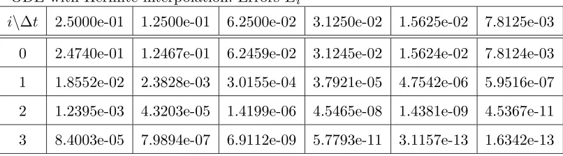
To observe this numerically we tabulate Ei, i = 0,1,2,3 for six values of ∆t
in Table 1 and Qi, i = 1,2,3 in Table 2. In Table 3 we see the convergence
predicted by the theory and Eq. (42). The interpolation error for Hermite interpolation is O(∆t4), which only begins to affect the convergence rates on
the 3rd iteration.
Table 1
ODE with Hermite interpolation: Errors Ei
i\∆t 2.5000e-01 1.2500e-01 6.2500e-02 3.1250e-02 1.5625e-02 7.8125e-03
0 2.4740e-01 1.2467e-01 6.2459e-02 3.1245e-02 1.5624e-02 7.8124e-03
1 1.8552e-02 2.3828e-03 3.0155e-04 3.7921e-05 4.7542e-06 5.9516e-07
2 1.2395e-03 4.3203e-05 1.4199e-06 4.5465e-08 1.4381e-09 4.5367e-11
Table 2
ODE with Hermite interpolation: RatiosQi=Ei/Ei 1
i\∆t 2.5000e-01 1.2500e-01 6.2500e-02 3.1250e-02 1.5625e-02 7.8125e-03
1 7.4985e-02 1.9112e-02 4.8279e-03 1.2137e-03 3.0428e-04 7.6181e-05
2 6.6811e-02 1.8131e-02 4.7086e-03 1.1990e-03 3.0250e-04 7.6226e-05
3 6.7774e-02 1.8493e-02 4.8675e-03 1.2711e-03 2.1665e-04 3.6022e-03
Table 3
ODE with Hermite interpolation: Estimated RatesQi(∆t)/Qi(2∆t)
i\∆t 1.2500e-01 6.2500e-02 3.1250e-02 1.5625e-02 7.8125e-03
1 2.5488e-01 2.5261e-01 2.5138e-01 2.5072e-01 2.5036e-01
2 2.7138e-01 2.5970e-01 2.5463e-01 2.5230e-01 2.5199e-01
3 2.7286e-01 2.6321e-01 2.6115e-01 1.7044e-01 1.6627e+01
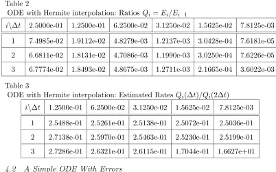
4.2 A Simple ODE With Errors
Here we repeat the computations from§4.1 under conditions more likely to be present in actual computations, i.e., the integration of the split equations and the operator estimates contain error. We introduce several types of error by: (1) replacing Hermite interpolation with linear interpolation; (2) increasing the tolerance of the ODE solver in both split equations; and (3) reducing the order and the accuracy of only the transport solve. The effect of any of these errors will be to increase the truncation error effects in Eqs. (24) and (25) and make Eq. (42) fail when the truncation error terms dominate the right sides of Eqs. (24) and (25).
4.2.1 Interpolation Error
We repeat the computations in §4.1, except now we use linear interpolation to estimate ˜Lr1 and ˜Lt over the transport and reaction solves, respectively. The error in linear interpolation isO(∆t2), the same order as the reduction in errors. As expected, we see interpolation effects in the second iteration, shown in the second row of Table 5.
4.2.2 Truncation Error
Table 4
ODE with linear interpolation: Errors Ei
i\∆t 2.5000e-01 1.2500e-01 6.2500e-02 3.1250e-02 1.5625e-02 7.8125e-03
0 2.4740e-01 1.2467e-01 6.2459e-02 3.1245e-02 1.5624e-02 7.8124e-03
1 1.2823e-02 1.9587e-03 2.7272e-04 3.6042e-05 4.6343e-06 5.8759e-07
2 2.7850e-04 2.3675e-05 2.0909e-06 1.6016e-07 1.1136e-08 7.3461e-10
3 8.7598e-04 5.3147e-05 3.2574e-06 2.0131e-07 1.2503e-08 7.7869e-10
Table 5
ODE with linear interpolation: Estimated Rates Qi(∆t)/Qi(2∆t)
i\∆t 1.2500e-01 6.2500e-02 3.1250e-02 1.5625e-02 7.8125e-03
1 3.0312e-01 2.7793e-01 2.6418e-01 2.5713e-01 2.5357e-01
2 5.5652e-01 6.3427e-01 5.7962e-01 5.4074e-01 5.2029e-01
3 7.1370e-01 6.9401e-01 8.0680e-01 8.9329e-01 9.4407e-01
First we repeat the computations of§4.1 usingatol=rtol = 10 4 in the ODE
solver ODE15s. The first row of Table 7 indicates that as (∆t) is reduced, the truncation error will begin to dominate, and second-order convergence is not evident. The ratio Qi(∆t)/Qi(2∆t) actually increases as (∆t) is decreased.
Table 6
ODE with solver tolerance = 10 4: ErrorsE i
i\∆t 2.5000e-01 1.2500e-01 6.2500e-02 3.1250e-02 1.5625e-02 7.8125e-03
0 2.4740e-01 1.2467e-01 6.2459e-02 3.1245e-02 1.5624e-02 7.8124e-03
1 1.8148e-02 2.3925e-03 3.3655e-04 1.0494e-04 4.8641e-05 2.0856e-05
2 1.1167e-03 1.8007e-04 1.5880e-04 1.0582e-04 4.8756e-05 2.0866e-05
3 1.3209e-04 1.7829e-04 1.5875e-04 1.0582e-04 4.8756e-05 2.0866e-05
Table 7
ODE with solver tolerance = 10 4: Estimated RatesQi(∆t)/Qi(2∆t)
i\∆t 1.2500e-01 6.2500e-02 3.1250e-02 1.5625e-02 7.8125e-03
1 2.6161e-01 2.8079e-01 6.2335e-01 9.2687e-01 8.5751e-01
2 1.2232e+00 6.2691e+00 2.1369e+00 9.9410e-01 9.9814e-01
3 8.3700e+00 1.0097e+00 1.0003e+00 1.0000e+00 1.0000e+00
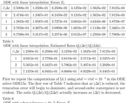
steps. To model this scenario, we repeat the calculations of §4.1 but solve the first step of the ISO algorithm (Eq. 3) using a second-order accurate integration method and adjust the solver tolerance such that the solution over the timestep ∆t is completed in only one or two substeps. The second step of the ISO algorithm (Eqs. 6–7) is computed using the same adaptive time stepping and tolerance used previously in §4.1. The rates in Table 9 show that we deviate from the second-order convergence, but the deviation appears smaller as (∆t) is decreased. This behavior was also observed in Table (5), where we reduced the interpolation accuracy.
Table 8
ODE with one low-order substep:Ei
i\∆t 2.5000e-01 1.2500e-01 6.2500e-02 3.1250e-02 1.5625e-02 7.8125e-03
0 2.4740e-01 1.2467e-01 6.2459e-02 3.1245e-02 1.5624e-02 7.8124e-03
1 1.8446e-02 2.8784e-03 4.2037e-04 5.7744e-05 7.6062e-06 9.7747e-07
2 3.7074e-04 5.3095e-05 5.4449e-06 4.4909e-07 3.2553e-08 2.1970e-09
3 1.4908e-03 1.1341e-04 8.1405e-06 5.5323e-07 3.6211e-08 2.3185e-09
Table 9
ODE with one low-order substep: Estimated RatesQi(∆t)/Qi(2∆t)
i\∆t 1.2500e-01 6.2500e-02 3.1250e-02 1.5625e-02 7.8125e-03
1 3.0966e-01 2.9151e-01 2.7460e-01 2.6341e-01 2.5701e-01
2 9.1776e-01 7.0221e-01 6.0044e-01 5.5029e-01 5.2517e-01
3 5.3118e-01 6.9994e-01 8.2396e-01 9.0297e-01 9.4873e-01
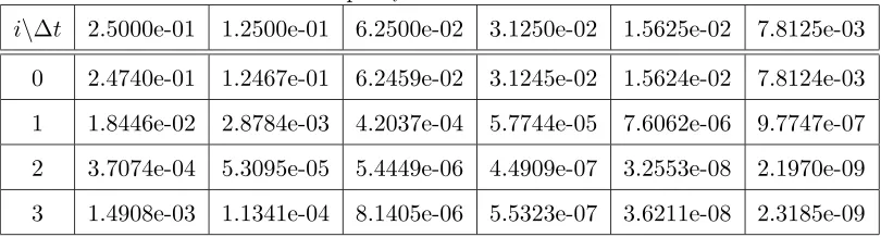
4.3 A More Complicated ODE
Many subsurface transport modeling efforts employ equilibrium mass transfer relationships that lead to an Rf that is not Lipschitz continuous near C = 0
[51]. The theoretical analysis assumes that Rf is Lipschitz, but one might ask
if this is a necessary condition. To investigate the sensitivity of the analysis to the Lipschitz assumption, we considered ODE systems with Rf(v) = 1/√v
andRf(v) = 1/(1 +v2). In the first case, theRf has a form that arises in
sub-surface modeling applications and for which the assumption of Lipschitz con-tinuity is violated. The second form is sufficiently smooth. One might expect that the first form degrades the ISO convergence rate while the second does not. The results for Rf(v) = 1/√v in Tables 10–11 and Rf(v) = 1/(1 +v2) in
Table 10
ODE withRf(v) = 1/√v: ErrorsEi
i\∆t 2.5000e-01 1.2500e-01 6.2500e-02 3.1250e-02 1.5625e-02 7.8125e-03
0 2.4740e-01 1.2467e-01 6.2459e-02 3.1245e-02 1.5624e-02 7.8124e-03
1 1.4964e-02 3.6734e-03 8.1460e-04 1.6783e-04 3.2646e-05 5.7186e-06
2 1.9867e-04 2.7798e-05 3.8206e-06 5.0851e-06 6.3568e-07 7.9464e-08
3 5.1079e-06 5.6116e-06 6.1460e-06 5.0852e-06 6.3569e-07 7.9465e-08
Table 11
ODE withRf(v) = 1/√v: Estimated RatesQi(∆t)/Qi(2∆t)
i\∆t 1.2500e-01 6.2500e-02 3.1250e-02 1.5625e-02 7.8125e-03
1 4.8714e-01 4.4265e-01 4.1186e-01 3.8898e-01 3.5033e-01
2 5.6996e-01 6.1980e-01 6.4600e+00 6.4267e-01 7.1363e-01
3 7.8519e+00 7.9684e+00 6.2166e-01 9.9999e-01 9.9999e-01
Table 12
ODE withRf(v) = 1/(1 +v2): ErrorsEi
i\∆t 2.5000e-01 1.2500e-01 6.2500e-02 3.1250e-02 1.5625e-02 7.8125e-03
0 2.4740e-01 1.2467e-01 6.2459e-02 3.1245e-02 1.5624e-02 7.8124e-03
1 2.4247e-02 2.6466e-03 3.1588e-04 3.8757e-05 4.8048e-06 5.9827e-07
2 2.7184e-03 5.9384e-05 1.6382e-06 4.8655e-08 1.4864e-09 4.6109e-11
3 2.9909e-04 1.3457e-06 8.7217e-09 6.4374e-11 3.3619e-13 1.6334e-13
Table 13
ODE withRf(v) = 1/(1 +v2): Estimated RatesQi(∆t)/Qi(2∆t)
i\∆t 1.2500e-01 6.2500e-02 3.1250e-02 1.5625e-02 7.8125e-03
1 2.1660e-01 2.3824e-01 2.4528e-01 2.4791e-01 2.4902e-01
2 2.0014e-01 2.3113e-01 2.4206e-01 2.4642e-01 2.4914e-01
3 2.0596e-01 2.3493e-01 2.4851e-01 1.7095e-01 1.5662e+01
4.4 A Nonlinear Reactive Transport Problem
4.4.1 Model Formulation
For convenience, we consider a model problem introduced in [29], which de-scribes solute transport, reaction, and interphase mass transfer in a porous medium system. Mass transfer occurs between a fluid phase and two types of solid phase—a fraction that achieves equilibrium quickly and a fraction that achieves equilibrium slowly. Transformation reactions are considered to be of a general form and may be linear or nonlinear. Subsets of this general model occur routinely in application, and because of this it makes a good test prob-lem for the solution issues of concern in this work. Because the major aspects of this work do not depend upon the spatial dimensionality of the system, we will restrict our efforts to one spatial dimension. We also limit ourselves to the case of transport with a known uniform flow field. This subset of the governing equations describing 1D transport in a uniform flow field is often employed for problems such as solute transport through soil columns, e.g. [17, 38, 20], fixed bed reactors, e.g. [3, 34, 46], and in many field-scale investigations, e.g. [1, 55, 60].
We formulate this model as
∂C ∂t +
ρb
θ ∂ωf
∂t =Dx ∂2C
∂x2 vx ∂C
∂x kaC
ra (43)
ρb
θ h
α(ωse ωs) +kfω rf
f
i
, in [0, Lx]×[0, ts]
∂ωs
∂t =α(ω
e
s ωs) ksωsrs, in [0, Lx]×[0, ts] (44)
subject to boundary conditions
C(0, t) =C0 (45)
∂C
∂x (Lx, t) = 0 (46)
and initial conditions
C(x,0) =sin
πx
Lx
(47)
ωs(x,0) = 0 (48)
where [0, Lx]⊂IR1 is the spatial domain; [0, ts] is the temporal domain;xand
tare the spatial and temporal coordinates, respectively;Cis an aqueous phase solute concentration; t is time; Dx is a hydrodynamic dispersion coefficient;
vx is a mean pore velocity; ka, kf, and ks are reaction rate constants for the
phase, respectively;ra,rf, andrsare reaction order exponents for the aqueous
phase, the rapidly sorbing solid phase, and the slowly sorbing solid phase, re-spectively;ρb is a solid-phase bulk density;αis a first-order mass transfer rate
coefficient for mass transfer between the aqueous phase and the slowly sorbing
solid phase; θ is porosity; ω is a mass averaged solid-phase solute
concentra-tion, i.e., mass fraction; ωf and ωs are solid-phase solute mass fractions for
the rapidly sorbing and slowly sorbing solid phase fractions, respectively; and
ωe, ωe
f and ωes are equilibrium solute mass fractions for the total, the rapidly
sorbing and slowly sorbing solid phase fraction, respectively, in equilibrium
with the aqueous-phase solute concentration Ce.
Equilibrium mass transfer between the fluid and solid phases is described by a combination of Freundlich equilibrium expressions
ωe=ωef +ωse (49)
ωe=Kf(Ce)nf +Ks(Ce)ns (50)
whereKf and Ks are Freundlich sorption capacity coefficients for the rapidly
sorbing and slowly sorbing solid-phase fraction, respectively; and nf and ns
are Freundlich exponents for the rapidly sorbing and slowly sorbing fraction, respectively.
The formulation summarized by Eqs. (43)–(50) is a coupled system of
nonlin-ear PDE’s in two primary dependent variables, C and ωs, if ωf is expressed
as a function ofC by invoking the assumption of local equilibrium. Eq. 43 is
frequently written in non-conservative form (e.g. [14, 23]) by assuming local equilibrium for the fast sites and using the chain rule to yield
Rf
∂C ∂t =Dx
∂2C
∂x2 vx
∂C
∂x kaC
ra (51)
ρb
θ h
α(ωse ωs) +kfω rf
f
i
, in Ω×[0, ts]
Rf= 1 +
ρb
θ ∂ωf
∂C (52)
where Rf is termed the retardation factor. We use this form of the equation
in this work.
In terms of the operator notation introduced§3, we have
Rf(C) = 1 +
ρb
θ KfnfC
nf 1 (53)
Lt(C) =Dx
∂2C
∂x2 vx
∂C
Lr1(C, ωs) = kaCra
ρb
θ [α(KsC
ns ωs) +k
fCrf] (55)
Lr2(C, ωs) =α(KsCns ωs) ksωrss (56)
4.4.2 Numerical Solution
We implemented the ISO algorithm using an approach in which the transport and reaction substeps are both solved using an ODE solver with formal er-ror control. The transport substep is solved using a method of lines (MOL) approach in which the spatial derivatives are approximated using a centered fi-nite difference to produce an ODE system for the concentrations at the nodes. This ODE system is integrated over [0,∆t] to a prescribed error tolerance using the stiff ODE solver ODE15s. The reaction substep consists of solving a local reaction problem over [0,∆t] at each node, again using ODE15s to produce a solution with a prescribed level of error.
We implemented several methods for computing the reaction operator estimate ˜
Lr1used in the transport substep, and the transport operator estimate ˜Ltused in the reaction substep. In the simplest approach these estimates were held constant over the respective substeps. Before the transport solve, the reaction operator estimateLr1 is computed using the current approximate solution. It
is then kept constant during the transport solve. Before the reaction solve, the transport operator estimate Lt is computed using the currrent approximate solution. It is then kept constant during the reaction solve. We implemented two approaches which represented ˜Lt and ˜Lr1 as functions of time. One
ap-proach uses linear interpolation between the current approximate solution and the solution at the begining of the time step. Another approach uses Hermite interpolation.
Based on the results in§4.3 for the non-LipschitzRf, we considered a technique that uses a smooth approximation of the Freundlich isotherm. The approach approximates ωe
f =Kf(Ce)nf with a cubic spline, using about 1000 points to cover the interval C ∈[0, C0]. Then Rf was computed using the derivative of the spline representation ofωe
f.
4.4.3 Numerical Experiments
In this instance no analytical solution is available. Therefore, our exact solu-tion is a numerical one computed with a MOL approach using the stiff ODE solver ODE15s. We selected this approach because it allows us to control the temporal error. We use this exact solution to compute the error in the ISO solution at each iteration. We compare the convergence over a single time step.
Table 14
Model Parameters
Dx vx ρb θ α Kf Ks ka kf ks
0.01 1 1.59 0.4 0.1 0.126 0.252 1 1 1
nf ns ra rf rs Lx ts C0 C0 ω0s
0.7 0.7 1 1 1 1 1 1 0 0
Numerical experiments were conducted for a single time step over a wide range of spatial and temporal discretizations. We considered the effect of in-terpolation accuracy for ˜Lt and ˜Lr1 on convergence by using constant, linear,
and Hermite interpolation. We observed results similar to those for the simple ODE problem, so they will not be shown here. In summary, we found that con-stant and linear interpolation both degraded the convergence rate to O(∆t), while Hermite interpolation of the operator estimates preserved the O(∆t2) convergence rate predicted by the analysis.
Tables 15–16 and 17–18 show the errors and convergence rate for the unsplined and splinedRf approaches, respectively, for 50 cell spatial discretization. Her-mite interpolation was used in both approaches, and ∆t = 1/2k for k = 6,7, . . . ,11. The exact solution and the substeps of the ISO solution were solved in MATLAB using the ODE15s code with relative and absolute er-ror tolerances set at 10 13. We observe that using the splined R
f approach preserves theO(∆t2) convergence rate.
Table 15
Model PDE with unsplinedRf approach: ErrorsEi
i\∆t 1.5625e-02 7.8125e-03 3.9062e-03 1.9531e-03 9.7656e-04 4.8828e-04
0 1.3289e-01 6.8916e-02 3.4932e-02 1.7561e-02 8.8004e-03 4.4048e-03
1 6.1164e-03 1.1270e-03 2.1160e-04 4.1161e-05 8.1896e-06 1.6388e-06
2 1.6587e-03 2.4611e-04 3.6634e-05 6.7019e-06 1.2379e-06 2.2518e-07
3 1.6622e-03 2.4636e-04 3.7587e-05 6.7780e-06 1.2441e-06 2.2566e-07
Table 16
Model PDE with unsplinedRf approach: Estimated RatesQi(∆t)/Qi(2∆t)
i\∆t 7.8125e-03 3.9062e-03 1.9531e-03 9.7656e-04 4.8828e-04
1 3.5530e-01 3.7041e-01 3.8696e-01 3.9702e-01 3.9980e-01
2 8.0524e-01 7.9281e-01 9.4046e-01 9.2836e-01 9.0900e-01
Table 17
Model PDE with splined Rf approach: Errors Ei
i\∆t 1.5625e-02 7.8125e-03 3.9062e-03 1.9531e-03 9.7656e-04 4.8828e-04
0 1.3289e-01 6.8916e-02 3.4932e-02 1.7561e-02 8.8004e-03 4.4048e-03
1 1.4244e-03 2.2490e-04 3.1539e-05 4.1739e-06 5.3679e-07 6.8058e-08
2 1.6587e-03 2.4611e-04 3.5803e-05 4.8263e-06 6.2645e-07 7.9793e-08
3 1.6622e-03 2.4636e-04 3.5812e-05 4.8266e-06 6.2646e-07 7.9794e-08
Table 18
Model PDE with splined Rf approach: Estimated RatesQi(∆t)/Qi(2∆t)
i\∆t 7.8125e-03 3.9062e-03 1.9531e-03 9.7656e-04 4.8828e-04
1 3.0445e-01 2.7666e-01 2.6326e-01 2.5662e-01 2.5331e-01
2 9.3971e-01 1.0374e+00 1.0186e+00 1.0093e+00 1.0046e+00
3 9.9892e-01 9.9924e-01 9.9980e-01 9.9995e-01 9.9999e-01
5 DISCUSSION
The analysis demonstrates that under fairly reasonable smoothness assump-tions, one can show that the theoretical convergence rate for ISO applied to our model NRTP’s is O∆t2, where ∆t is the time step of the numerical method. This result is independent of the class of spatial discretization em-ployed and is valid in 1D, 2D, or 3D domains. The theory does assume that the relevant temporal integration of the split equations can be done as accu-rately as needed. Obviously, this assumption must be relaxed in practice and may result in slower convergence in real applications.
Numerical experiments on a simple ODE system indicate that several factors may reduce the convergence rate of ISO in practice. We observed that reducing the accuracy used in the integration of the split equations has an adverse effect on the order of convergence. We also observed that reducing the accuracy of the interpolation used in the operator estimates can lower the convergence rate.
[42, 59, 71], it has significant implications for solving realistic problems.
Numerical experiments using an ODE with a model Rf term lend insight
into the importance of the Lipschitz continuity assumption used in the anal-ysis. The analysis treats Lipschitz continuity as a sufficient condition, but the numerical experiments indicate that it may be a necessary condition. This has significant practical implications for subsurface transport investigations, since the Freundlich model for sorption equilibrium often used in subsurface
transport simulations results in an Rf which is non-Lipschitz for very low
concentrations. The Freundlich model does not reduce to a linear relationship
between C and ω at low fluid-phase concentrations. Instead,∂ω/∂C tends to
infinity as the fluid phase solute concentration approaches zero.
The results of the numerical experiments on the model NRTP show that one can implement the ISO algorithm in a manner that preserves the second-order convergence predicted by the theory. Simple constant or linear approximations for the transport and reaction operator estimates destroy the second-order convergence rate, while Hermite interpolation along with a smooth approxi-mation for the retardation factor preserve second-order convergence. We stress that we looked at convergence, and we have not systematically investigated the computational efficiency of this approach. If the work for each iteration of the ISO method is excessive, it may not be competitive with other SO approaches or with the best FC approaches. This is an area which deserves further research.
6 CONCLUSIONS
Based upon the analysis and numerical experiments, We draw several conclu-sions regarding the use of the ISO algorithm for NRTP’s:
(1) Theoretical analysis shows that, given certain assumptions regarding smooth-ness, the rate of convergence for ISO solution of NRTP’s isO(∆t2).
(2) Numerical experiments using a simple ODE system indicate that the the-oretical convergence rate can be degraded by discretization errors intro-duced into the numerical solution and by coarse estimates of the reaction and transport operators. Experiments on ODE models also imply that Lipschitz continuity is an important assumption in practice.
(3) Numerical experiments on a model PDE system using typical finite dif-ference implementations of the ISO approach (i.e., with constant and linear estimates of the reaction and transport operators) and using the Freundlich sorption equilibrium model agree with the results of ODE experiments.
transport and reaction operator estimates, and using a smooth approxi-mation to the Freundlich sorption model, one can obtain the theoretical rate of convergence.
(5) Additional research on the computational efficiency of the the ISO ap-proach introduced here is needed before it is proposed for routine sub-surface simulation projects.
Acknowledgements
The UNC aspects of this work have been supported by the National Institute of Environmental Health Sciences (NIEHS) grant 5 P42 ES05948-02 and the National Science Foundation (NSF) grant DMS-0112653. The work at NCSU has been supported by NSF grants DMS-0070641 and DMS-0112542, and the US Army Research Office (ARO) grant DAAD19-99-1-0186. Computational support was provided by the North Carolina Supercomputer Center and from Cray Research, Inc.
References
[1] R.H. Abrams and K. Loague. A compartmentalized solute transport model for redox zones in contaminated aquifers, 2. Field-scale simulations.
Water Resources Research, 36(8):2015–2029, 2000.
[2] C. A. J. Appelo and A. Willemsen. Geochemical calculations and obser-vations on salt water intrusions, I. A combined geochemical/mixing cell model. Journal of Hydrology, 94:313–330, 1987.
[3] A. K. Avci, D. L. Trimm, and Z. I. Onsan. Heterogeneous reactor model-ing for simulation of catalytic oxidation and steam reformmodel-ing of methane.
Chemical Engineering Science, 56(2):641–649, 2001.
[4] D. A. Barry. Supercomputers and their use in modeling subsurface solute transport. Reviews of Geophysics, 38(3):277–295, 1990.
[5] D. A. Barry, C. T. Miller, P. J. Culligan, and K. Bajracharya. Split operator methods for reactive chemical transport in groundwater. In Proceeding of the International Conference on Modeling and Simulation
1995: MODSIM95, pages 125–132, New South Wales, 1995. Modeling and
Simulation Society of Australia, Inc.
[6] D. A. Barry, C. T. Miller, P. J. Culligan, and K. Bajracharya. Analysis of split operator methods for nonlinear and multispecies groundwater chemical transport models. Mathematics and Computers in Simulation, 43:331–341, 1997.
reaction/groundwater transport models.Journal of Contaminant Hydrol-ogy, 22(1/2):1–17, 1996.
[8] D.A. Barry, K. Bajracharya, M. Crapper, H. Prommer, and C.J. Cunning-ham. Comparison of split-operator methods for solving coupled chemical
non-equilibrium reaction/groundwater transport models. Mathematics
and Computers in Simulation, 53:113–127, 2000.
[9] I. Bey, D.J. Jacob, R.M. Yantosca, J.A. Logan, B.D. Field, A.M. Fiore, Q.B. Li, H.G.Y. Liu, L.J. Mickley, and M.G. Schultz. Global modeling of tropospheric chemistry with assimilated meteorology: Model description
and evaluation. Journal of Geophysical Research-Atmospheres, 106(D19):
23073–3095, 2001.
[10] D. Bhuyan, L. W. Lake, and G. A. Pope. Mathematical modeling of
high-pH chemical flooding. SPE Reservoir Engineering, 5:213–220, 1990.
[11] J.G. Blom and J.G. Verwer. A comparison of integration methods for
atmospheric transport-chemistry problems. Journal of Computational
and Applied Mathematics, 126(1–2):381–396, 2000.
[12] M. Blunt, F. J. Fayers, and F. M. Orr. Carbon-dioxide in enhanced
oil-recovery. Energy Conversion and Management, 34(9–1):1197–1204, 1992.
[13] R. C. Borden, P. B. Bedient, M. D. Lee, C. H. Ward, and J. T. Wil-son. Transport of dissolved hydrocarbons influenced by oxygen-limited
biodegradation, 2. Field application. Water Resources Research, 22(13):
1983–1990, 1986.
[14] M. L. Brusseau and P. S. C. Rao. Sorption nonideality during organic
con-taminant transport in porous media. Critical Reviews in Environmental
Control, 19(1):33–99, 1989.
[15] M. A. Celia, J. S. Kindred, and I. Herrera. Contaminant transport and biodegradation 1. A numerical model for reactive transport in porous
media. Water Resources Research, 25(6):1141–1148, 1989.
[16] H. P. Cheng and G. T. Yeh. Development and demonstrative application of a 3-D numerical model of subsurface flow, heat transfer, and reactive
chemical transport: 3DHYDROGEOCHEM.Journal of Contaminant
Hy-drology, 34(1–2):47–83, 1998.
[17] C. V. Chrysikopoulos, P. K. Kitanidis, and P. V. Roberts. Analysis of one-dimensional solute transport through porous media with spatially
variable retardation factor. Water Resources Research, 26(3):437–446,
1990.
[18] S.P. Chu and H. Elliott. Latitude versus depth simulations of ecodynamics and dissolved gas chemistry relationships in the central pacific. Journal of Atmospheric Chemistry, 40(3):305–333, 2001.
[19] D.M. Cooper, A. Jenkins, R. Skeffington, and B. Gannon. Catchment-scale simulation of stream water chemistry by spatial mixing: Theory and
application. Journal of Hydrology, 233(1–4):4121–137, 2000.
[20] B. B. Dykaar and P. K. Kitanidis. Macrotransport of a biologically
re-acting solute through porous media. Water Resources Research, 32(2):
[21] P. Engesgaard and K. L. Kipp. A geochemical transport model for redox-controlled movement of mineral fronts in groundwater flow systems — A case of nitrate removal by oxidation of pyrite. Water Resources Research, 28(10):2829–2843, 1992.
[22] P. Engesgaard and R. Traberg. Contaminant transport at a waste residue
deposit. 2. Geochemical transport modeling. Water Resources Research,
32(4):939–951, 1996.
[23] T. C. Harmon, W. P. Ball, and P. V. Roberts. Nonequilibrium transport of organic contaminants in groundwater. In B. L. Sawhney and K. Brown,
editors, Reactions and Movement of Organic Chemicals in Soils, pages
405–438. Soil Science Society of America, Inc., Madison, Wisconsin, 1989. [24] J. Herzer and W. Kinzelbach. Coupling of transport and chemical
pro-cesses in numerical transport models. Geoderma, 44:115–127, 1989.
[25] K.S. Hunter, Y.F. Wang, and P.M. Van Cappellen. Kinetic modeling of microbially-driven redox chemistry of subsurface environments: Coupling
transport, microbial metabolism and geochemistry. Journal of Hydrology,
209(1–4):53–80, 1998.
[26] M.Z. Jacobson. Fundamentals of Atmospheric Modeling. Cambridge
Uni-versity Press, 1998.
[27] A. A. Jennings, D. J. Kirkner, and T. L. Theis. Multicomponent
equi-librium chemistry in groundwater quality models. Water Resources
Re-search, 18(4):1089–1096, 1982.
[28] J. J. Kaluarachchi and J. Morshed. Critical assessment of the operator splitting technique in solving the advection dispersion reaction equation. 1. First-order reaction. Advances in Water Resources, 18(2):89–100, 1995. [29] J. F. Kanney, C. T. Miller, and D. A. Barry. Comparison of fully coupled approaches for approximating nonlinear transport and reaction problems. Advances in Water Resources, (In Press), 2002.
[30] J. Kim and S. Y. Cho. Computation accuracy and efficiency of the time-splitting method in solving atmospheric transport-chemistry equations. Atmospheric Environment, 31(15):2215–2224, 1997.
[31] A.A. Koelmans, A. Van der Heijde, L.M Knijff, and R.H. Aalderink. In-tegrated modelling of eutrophication and organic contaminant fate &
ef-fects in aquatic ecosystems. A review. Water Research, 35(15):3517–3536,
2001.
[32] R. Kopmann and Markofsky M. Three-dimensional water quality
mod-elling with TELEMAC-3D. Hydrological Processes, 14(13):2279–2292,
2000.
[33] A.S. Koziol and J.A. Pudykiewicz. Global-scale environmental transport
of persistent organic pollutants. Chemosphere, 45(8):1181–1200, 2001.
[34] S. Krishnaswamy, R.D. Gunn, and P.K. Agarwal. Low-temperature ox-idation of coal, 2. An experimental and modelling investigation using a fixed-bed isothermal flow reactor. Fuel, 75(3):344–352, 1996.
[35] L. W. Lake. Enhanced Oil Recovery. Prentice Hall, Englewood Cliffs, NJ,
[36] D. Lanser and Verwer J.G. Analysis of operator splitting for advection-diffusion-reaction problems from air pollution modelling.Journal of
Com-putational and Applied Mathematics, 111(1–2):201–216, 1999.
[37] R. J. LeVeque and J. Oliger. Numerical methods based on additive
split-tings for hyperbolic partial differential equations. Mathematics of
Com-putation, 40(162):469–497, 1983.
[38] D. M. Linn. Sorption and Degradation of Pesticides and Organic
Chem-icals in Soil. Soil Science Society of America, Inc., and American Society of Agronomy, Inc., Madison, WI, 1993.
[39] C. W. Liu and T. N. Narasimhan. Redox-controlled multiple-species
reac-tive chemical transport 1. Model development.Water Resources Research,
25(5):869–882, 1989.
[40] K. T. MacQuarrie, E. A. Sudicky, and E. O. Frind. Simulation of
biodegradable organic contaminants in groundwater, 1. Numerical formu-lation in principal directions. Water Resources Research, 26(2):207–222, 1990.
[41] A. Mahadevan and D. Archer. Modeling the impact of fronts and
mesoscale circulation on the nutrient supply and biogeochemistry of the
upper ocean. Journal of Geophysical Research-Oceans, 105(C1):1209–
1225, 2000.
[42] W. W. Mcnab and T. N. Narasimhan. A multiple species transport model with sequential decay chain interactions in heterogeneous subsurface
en-vironments. Water Resources Research, 29(8):2737–2746, 1993.
[43] G. J. McRae, W. R. Goodin, and J. H. Seinfeld. Numerical solution of the atmospheric diffusion equation for chemically reacting flows. Journal of Computational Physics, 45:1–42, 1982.
[44] C. T. Miller, G. Christakos, P. T. Imhoff, J. F. McBride, J. A. Pedit, and J. A. Trangenstein. Multiphase flow and transport modeling in
hetero-geneous porous media: Challenges and approaches. Advances in Water
Resources, 21(2):77–120, 1998.
[45] C. T. Miller and A. J. Rabideau. Development of split-operator,
Petrov-Galerkin methods to simulate transport and diffusion problems. Water
Resources Research, 29(7):2227–2240, 1993.
[46] P. Mizsey, A. Cuellar, E. Newson, P. Hottinger, T. Truong, and F. von Roth. Fixed bed reactor modelling and experimental data for catalytic
dehydrogenation in seasonal energy storage applications. Computers &
Chemical Engineering, 23:S379–S382, 1999.
[47] J. Morshed and J. J. Kaluarachchi. Critical assessment of the operator splitting technique in solving the advection dispersion reaction equation
2. Monod kinetics and coupled transport. Advances in Water Resources,
18(2):101–110, 1995.
[48] D.J. Mossman and N. AlMulki. One-dimensional unsteady flow and un-steady pesticide transport in a reservoir. Ecological Modelling, 89(1–3): 259–267, 1996.
Elsevier, New York, 1987.
[50] D.L. Parkhurst. User’s Guide to PHREEQC: A Computer Program for
Speciation, Reaction-Path, Advective-Transport and Diffusion Problems.
U.S. Geological Survey, 1995. Water Resource Investigation Report 95-4227.
[51] J. A. Pedit. An investigation of heterogeneous sorption by a natural solid. PhD thesis, University of North Carolina, Chapel Hill, NC, 1994.
[52] G. A. Pope and M. Bavi`ere. Basic Concepts in Enhanced Oil Recovery
Processes. Elsevier, New York, 1991.
[53] H. Prommer, D. A. Barry, and G. B. Davis. A one-dimensional reactive multi-component transport model for biodegradation of petroleum
hy-drocarbons in groundwater. Environmental Modelling and Software, 14:
213–223, 1999.
[54] H. Prommer, G.B. Davis, and D.A. Barry. PHT3D – A three-dimensional biogeochemical transport model for modelling natural and enhanced
re-memdiation. In C.D. Johnston, editor, Contaminated Site Remediation:
Challenges Posed by Urban and Industrial Contaminants, pages 351–358,
Fremantle, WA, 21-25 March 1999.
[55] F. Rocha and A. Walker. Simulation of the persistence of atrazine in soil at different sites in portugal. Weed Research, 35:179–186, 1995.
[56] J. Rubin. Transport of reacting solutes in porous media: Relation be-tween mathematical nature of problem formulation and chemical nature
of reactions. Water Resources Research, 19(5):1231–1252, 1983.
[57] R.L. Runkel, K.E. Bencala, R.E. Broshears, and S.C. Chapra. Reac-tive solute transport in streams. 1. Development of an equilibrium-based
model. Water Resources Research, 32(2):409–418, 1996.
[58] M.W. Saaltink, J. Carrera, and C. Ayora. On the behavior of approaches
to simulate reactive transport. Journal of Contaminant Hydrology, 48:
213–235, 2001.
[59] D. Schafer, W. Schafer, and W. Kinzelbach. Simulation of reactive pro-cesses related to biodegradation in aquifers. 1. Structure of the
three-dimensional reactive transport model. Journal of Contaminant
Hydrol-ogy, 31(1–2):167–186, 1998.
[60] T.D. Scheibe, Y.J. Chien, and J.S. Radtke. Use of quantitative models
to design microbial transport experiments in a sandy aquifer. Ground
Water, 39(2):210–222, 2001.
[61] L. F. Shampine and M. W. Reichelt. The MATLAB ODE suite. SIAM
Journal of Scientific Computing, 18(1):1–22, 1997.
[62] J. Simunek and D. L. Suarez. Two-dimensional transport model for
vari-ably saturated porous media with major ion chemistry. Water Resources
Research, 30(4):1115–1133, 1994.
[63] H.B. Singh. Composition, Chemistry, and Climate of the Atmosphere.
John Wiley and Sons, New York, 1995.
Environmen-tal Modelling and Software, 15(6–7):673–679, 2000.
[65] C. I. Steefel and K. T. B. MacQuarrie. Approaches to modeling of reactive transport in porous media. In P. C. Lichtner, C. I. Steefel, and E. H.
Oelkers, editors,Reactive Transport in Porous Media: General Principles
and Applications to Geochemical Processes, pages 83–129. Mineralogical
Society of America, Washington, DC, 1996.
[66] C. I. Steefel and S.B. Yabusaki. OS3D/GIMRT, Software for Modelling
Multicomponent-Multidimensional Reactive Transport, User Manual and
Programmer’s Guide. Pacific Northwest Laboratory, Richland,
Washing-ton, 1995.
[67] D.L. Stefanovic and H.G. Stefan. Accurate two-dimensional simulation of advective-diffusive-reactive transport. Journal of Hydraulic
Engineering-ASCE, 127(9):728–737, 2001.
[68] G. Strang. On the construction and comparison of difference schemes.
SIAM Journal on Numerical Analysis, 5(3):506–517, 1968.
[69] N.-Z. Sun. Mathematical Modeling of Groundwater Pollution.
Springer-Verlag, New York, 1996.
[70] A. J. Valocchi and M. Malmstead. Accuracy of operator splitting for
advection-dispersion-reaction problems. Water Resources Research, 28
(5):1471–1476, 1992.
[71] A. L. Walter, E. O. Frind, D. W. Blowes, C. J. Ptacek, and J. W. Molson. Modeling of multicomponent reactive transport in groundwater 1. Model
development and evaluation. Water Resources Research, 30(11):3137–
3148, 1994.
[72] K.Y. Wang, J.A. Pyle, and D.E. Shallcross. Formulation and evaluation of ims, an interactive three-dimensional tropospheric chemical transport
model 1. Model emission schemes and transport processes. Journal of
Atmospheric Chemistry, 38(2):195–227, 2001.
[73] M. F. Wheeler and C. N. Dawson. An operator-splitting method for advection-diffusion-reaction problems. Technical Report Technical Re-port 87-9, Rice University Department of Computational and Applied Mathematics, Houston, TX, 1987.
[74] M. F. Wheeler, C. N. Dawson, P. B. Bedient, C. Y. Chiang, R. C. Borden, and H. S. Rifai. Numerical simulation of microbial biodegradation of
hydrocarbons in ground water. InProceedings of the NWWA Conference
on Solving Ground Water Problems with Models, pages 92–109, 1987.
[75] T. M. Wood and A. M. Baptista. A model for diagnostic analysis of
estuarine geochemistry. Water Resources Research, 29(1):51–71, 1993.
[76] T. Xu, J. Samper, C. Ayora, M. Manzano, and E. Custidio. Modeling of non-isothermal multi-component reactive transport in field scale porous
media flow systems. Journal of Hydrology, 214(1–4):144–164, 1999.
[77] G. T. Yeh and V. S. Tripathi. A critical evaluation of recent develop-ments in hydrogeochemical transport models of reactive multichemical
components. Water Resources Research, 25(1):93–108, 1989.
multispecies components: Model development and demonstration. Water
Resources Research, 27(12):3075–3094, 1991.
[79] A. Zysset and F. Stauffer. Modeling of microbial processes in groundwa-ter infiltration systems. In T. F. Russell, R. E. Ewing, C. A. Brebbia,
W. G. Gray, and G. F. Pinder, editors, Mathematical Modeling in Water
Resources, volume 2, pages 325–332, Southampton, UK, 1992.
Computa-tional Mechanics Publications.
[80] A. Zysset, F. Stauffer, and T. Dracos. Modeling of chemically
reac-tive groundwater transport. Water Resources Research, 30(7):2217–2228,