Model-free Variable Selection in Reproducing Kernel Hilbert
Space
Lei Yang [email protected]
Department of Population Health New York Univeristy
New York, NY, 10016, USA
Shaogao Lv [email protected]
Center of Statistics
Southwestern University of Finance and Economics Chengdu, Sichuan, 610074, China
Junhui Wang [email protected]
Department of Mathematics City University of Hong Kong Kowloon Tong, 999077, HongKong
Editor:Jie Peng
Abstract
Variable selection is popular in high-dimensional data analysis to identify the truly informa-tive variables. Many variable selection methods have been developed under various model assumptions. Whereas success has been widely reported in literature, their performances largely depend on validity of the assumed models, such as the linear or additive models. This article introduces a model-free variable selection method via learning the gradient functions. The idea is based on the equivalence between whether a variable is informative and whether its corresponding gradient function is substantially non-zero. The proposed variable selection method is then formulated in a framework of learning gradients in a flex-ible reproducing kernel Hilbert space. The key advantage of the proposed method is that it requires no explicit model assumption and allows for general variable effects. Its asymptotic estimation and selection consistencies are studied, which establish the convergence rate of the estimated sparse gradients and assure that the truly informative variables are correctly identified in probability. The effectiveness of the proposed method is also supported by a variety of simulated examples and two real-life examples.
Keywords: group Lasso, high-dimensional data, kernel regression, learning gradients, reproducing kernel Hilbert space (RKHS), variable selection
1. Introduction
In literature, a wide spectrum of variable selection methods have been proposed based on various model assumptions. For example, under the linear model assumption, regular-ized regression models are popularly used for variable selection, including the nonnegative garrote (Breiman and Friedman, 1985), the least absolute shrinkage and selection operator (Tibshirani, 1996), the smoothly clipped absolute deviation (Fan and Li, 2001), the adap-tive Lasso (Zou, 2006), the combinedL0 andL1 penalty (Liu and Wu, 2007), the truncated L1 penalty (Shen et al., 2012), and many others. The main strategy is to associate the least square loss function with a sparsity-inducing penalty, leading to sparse representation of the resultant regression function. With the linear regression model, the sparse representation leads to variable selection based on whether the corresponding regression coefficient is zero. The aforementioned variable selection methods have demonstrated superior performance in many real applications. Yet their success largely relies on the validity of the linear model assumption. To relax the model assumption, attempts have been made to extend the variable selection methods to a nonparametric regression context. For example, under the additive regression model assumption, a number of variable selection methods have been developed (Shively et al., 1999; Huang and Yang, 2004; Xue, 2009; Huang et al., 2010). Furthermore, higher-order additive models can be considered, allowing each func-tional component contain more than one variables, such as the component selection and smoothing operator (Cosso) method (Lin and Zhang, 2006). While this method provides a more flexible and still interpretable model compared to the classical additive models, the number of functional components increases exponentially with the dimension. Another stream of research on variable selection is to conduct screening (Fan et al., 2011; Zhu et al., 2011; Li et al., 2012), which treats each individual variable separately and assures the sure screening properties. To overcome the issue of ignoring interaction effects, a higher-order interaction screening method is also developed (Hao and Zhang, 2014). Model-free variable selection has also been approached in the context of sufficient dimension reduction (Li et al., 2005; Bondell and Li, 2009). More recently, Stefanski et al. (2014) introduced a novel measurement-error-model-based variable selection method that can be adapted to a nonparametric kernel regression.
In this article, we propose a novel model-free variable selection method, which requires no explicit model assumptions and allows for general variable effects. The method is based on the idea that a variable is truly informative with respect to the regression function if the gradient of the regression function along the corresponding coordinate is substantially different from zero. Thus the proposed variable selection method is formulated in a gradi-ent learning framework equipped with a flexible reproducing kernel Hilbert space (Wahba, 1999). Learning gradients can be traced back to H¨ardle and Gasser (1985). Some of its recent developments include Jarrow et al. (2004), Mukherjee and Zhou (2006), Ye and Xie (2012), and Brabanter et al. (2013), where the main focus is to estimate the gradient functions.
simultaneously. Specifically, the proposed variable selection method via gradient learning is formulated in a regularization form that consists of a pairwise loss function for estimating the gradient functions and a group Lasso penalty.
One of the main features of the proposed variable selection method is that it does not require any explicit model assumption and detect informative variables with various effects on the regression function. This is a major advantage over most existing model-based variable selection methods which need to pre-specify a working model. If higher-order variable effects are considered, the model-based methods need to enumerate the possible components, whose number increases exponentially with the dimensionp. In sharp contrast, our proposed method only needs to estimate p components, while allowing for general variable effects.
Another interesting feature of the proposed method is the use of coefficient-based rep-resentation in estimating the gradient function. It follows directly from the representor theorem (Wahba, 1999) in a RKHS, and turns out to greatly facilitate variable selection in the gradient learning framework. With the coefficient-based representation, the group Lasso penalty can be naturally enforced on all the coefficients associated with the same variable. This leads to a well-structured optimization task, and can be efficiently solved through a blockwise coordinate descent algorithm (Yang and Zou, 2015). This is contrast to the exist-ing gradient learnexist-ing methods such as Ye and Xie (2012), where standard RHKS is used and a squared RKHS-norm penalty is enforced to attain the sparsity structure in the estimated gradients, and a forward-backward splitting algorithm is required for computation.
Finally, the effectiveness of the proposed method is supported by a variety of simulated and real examples. More importantly, its asymptotic estimation and selection consisten-cies are established, showing that the proposed method shall recover the truly informative variables with probability tending to one, and estimate the true gradient function at a fast convergence rate. Note that the variable selection consistency is not established in Ye and Xie (2012), and the estimation consistency of our method is more challenging due to the additional hypothesis error arises in the coefficient-based formulation. Also, as in many nonparametric variable selection methods (Lin and Zhang, 2006; Xue, 2009; Huang et al., 2010), the results are obtained in the sneario of fixed dimension, which are particlarly inter-esting given the fact that the variable selection consistency is obtained without assuming any explicit model.
The rest of the article is organized as follows. Section 2 presents a general framework of the proposed model-free variable selection method as well as an efficient computing al-gorithm to tackle the resultant large-scale optimization task. Section 3 establishes the asymptotic results of the proposed method in terms of both estimation and variable se-lection. The numerical experiments on the simulated examples and real applications are contained in Section 4. A brief discussion is provided in Section 5, and the Appendix is devoted to the technical proofs.
2. Model-free variable selection
2.1 Preambles
the following regression model,
y =f∗(x) +,
where E(|x) = 0, Var(|x) = σ2,x = (x(1), . . . , x(p))T is supported on a compact metric space X, and f∗ is the true regression function that is assumed to be twice differentiable everywhere.
When p is large, it is generally believed that only a small number of variables are truly informative. In literature, to define the truly informative variables, f∗ is often assumed to be of certain form. For instance, if f∗(x) = xT β∗
with β∗ = (β∗1, . . . , βp∗)T, then x(j) is regarded as truly informative if βj∗ 6= 0. However, this linear model assumption on f∗ can be too restrictive in practice, and whether a variable is informative shall not depend on the assumed model. In this article, a model-free variable selection method is developed without assuming any explicit form forf∗.
Since no explicit form is assumed forf∗, we note that ifx(l)is non-informative inf∗, the corresponding gradient function∇fl∗(x) =∂f∗(x)/∂x(l)≡0 for any x. This fact motivates the proposed model-free variable selection method in a gradient learning framework. Denote g∗(x) = ∇f∗(x) = (∇f∗
1(x), . . . ,∇fp∗(x))T the true gradient function, and the estimation error as
E(g) = E(x,y),(u,v)w(x,u)(y−v−g(x)T(x−u))2
= 2σs2+Ex,uw(x,u)(f∗(x)−f∗(u)−g(x)T(x−u))2, (1)
where σs2 = E(x,y),(u,v)[w(x,u)(y−f∗(x))2] is independent of g, and w(x,u) is a weight function that decreases as kx−uk increases and ensures the local neighborhood ofx con-tributes more to estimating g∗(x). Typically, w(x,u) =e−kx−uk2/τ2
n with a pre-specified
positive parameterτn2, which plays a key role in the asymptotic estimation consistency and is to be elaborated.
2.2 Coefficient-based formulation
Given the training set (xi, yi); i= 1, . . . , n, E(g) is approximated by its empirical version, and then the proposed variable selection method is formulated as
argmin
g∈Hp K
s(g) = 1 n(n−1)
n X
i,j=1 wij
yi−yj−g(xi)T(xi−xj) 2
+J(g), (2)
where wij = w(xi,xj), HK denotes a RKHS induced by a pre-specified kernel K(·,·), J(g) = λnPp
l=1πlJ(gl) is a penalty function on the complexity of g, and πl’s are the adaptive tuning parameters to be specified. The representor theorem assures that the minimizer of (2) must be of the following coefficient-based representation,
gl(x) = n X
t=1
αltK(x,xt); l= 1, . . . , p.
between ridge regression with a coefficient-based representation and support vector machine (Cortes and Vapnik, 1995) is also established in Scholk¨opf and Smola (2002).
Furthermore, to exploit the sparse structure in the regression model, we propose to consider the following sparsity-inducing penalty,
J(gl) = inf n
kα(l)k2 :gl(·) = n X
t=1
αltK(·,xt) o
. (3)
Here the group Lasso type of penalty kα(l)k2 attains the effect of pushing all or none of αtl’s to be exactly 0 and thus achieves the purpose of variable selection. The infimum is necessary for defining the penalty as the kernel basis {K(·,xt)}n
t=1 may not be linearly independent and thus the representation ofglinHK may not be unique. This penalty term differs from that in Ye and Xie (2012) in that our coefficient-based penalty does not rely on K and usually leads to sparser solutions. On the contrary, the penaltykglkK in Ye and Xie (2012) can be sensitive to the choice of K as its minimum eigenvalue can be very small. In addition, the finite dimensional hypothesis space is more flexible than the standard RHKS, and particularly the positive definiteK is no longer needed. This relaxation can be critical in scenarios when such kernels are inappropriate.
With the coefficient-based representation and the group Lasso penalty, the proposed variable selection formulation can be rewritten as
argmin
α(1),...,α(p) 1 n(n−1)
n X
i,j=1 wij
yi−yj−
p X
l=1
KTi α(l)(xil−xjl) 2
+λn p X
l=1
πlkα(l)k2, (4)
where Ki = (K(xi,x1), . . . , K(xi,xn))T is the i-th column of K = (K(xi,xj))n×n, and λn is a tuning parameter. The infimum operator in (3) is absorbed in the minimization in (4). Clearly, (4) simplifies the original formulation (2) from a functional space to a finite-dimensional vector space. However, the vector space is of dimensionnp and thus still requires an efficient large-scale optimization scheme, which will be developed in the next section.
2.3 Computing algorithm
To solve (4), we develop a block coordinate descent algorithm as in Yang and Zou (2015). First, after dropping theα-unrelated terms, the cost function in (4) can be simplified as
argmin
α −α
T U+1
2α T
Mα+λn p X
l=1
πlkα(l)k2, (5)
whereαT = (α(1))T, . . . ,(α(p))T
,U= n(n2−1)Pn
i,j=1wijUij,M= n(n2−1)Pni,j=1wijMij, Uij = (yi−yj)(xi−xj)⊗Ki,
Mij =
(xi−xj)(xi−xj)T
⊗ KiKTi ,
Then we update one α(l) at a time pretending others fixed, and the l-th subproblem becomes
argmin
α(l)
L(α) +λnπlkα(l)k2 =−α T
U+1 2α
T
Mα+λnπlkα(l)k2,
To solve the subproblem, a similar approximation as in Yang and Zou (2015) can be em-ployed, where the updatedα(l) is obtained by solving
argmin
α(l)
∇lL(αe)(α(l)−αe(l)) +γ (l) 2 (α
(l)− e
α(l))T(α(l)−αe(l)) +λnπlkα(l)k2. (6)
Here αe is the current estimate forα,αe
(l) is thel-th column of e α,
∇L(αe) = 2 n(n−1)
n X
i,j=1
wij(Mijαe−Uij),
∇lL(αe) denotes thel-th block vector of∇L(αe), and
∇lL(αe) = 2 n(n−1)
n X
i,j=1 wij
p X
s=1
((xi−xj)(xi−xj)T)lsKiKTi αe
(s)−(y
i−yj)(xil−xjl)Ki !
,
where ((xi−xj)(xi−xj)T)ls is the (l, s)-th entry of (xi −xj)(xi−xj)T. Furthermore, denote γ(l) the largest eigenvalue of
M(l)= 2 n(n−1)
n X
i,j=1
wij((xi−xj)(xi−xj)T)llKiKTi ,
which is thel-thn×nblock diagonal ofM.
It is straightforward to show that (6) has an analytical solution,
α(l)=
e
α(l)−∇lL(αe) γ(l)
1− λnπl kγ(l)
e
α(l)− ∇lL(αe)k2 !
+
. (7)
The proposed algorithm then iteratively updates α(l) for l = 1, . . . , p,1, . . . until conver-gence. The algorithm is guaranteed to converge to the global minimum, since the cost function in (5) is convex and its value is decreased in each updating step. Furthermore, the computational complexity of the block coordinate descent algorithm is O(n2p2D) with D being the number of iterations until convergence, which can be substantially less than the complexity of solving (5) with standard optimization packages.
3. Asymptotic theory
This section presents the asymptotic estimation and variable selection consistencies of the proposed model-free variable selection method. The estimation consistency assures that the distance between ˆg and g∗ converges to 0 at a fast rate, and the variable selection
tending to 1. Both consistency results are established for fixed p. For simplicity, we as-sume only the firstp0 variablesx(1), . . . , x(p0)are truly informative. The following technical assumptions are made.
Assumption A1. The support X is a non-degenerate compact subset of Rp, and there exists a cosntatnt c1 such that supxkH∗(x)k2 ≤ c1, where H∗(x) = ∇2f∗(x). Also, supx|K(x,x)|= 1, and the largest eigenvalue of Kis of order O(nψ) with 0≤ψ≤1.
Assumption A2. For some constants c2 and θ > 0, the probability density p(x) exists and satisfies
|p(x)−p(u)| ≤c2dX(x,u)θ, for any x,u∈ X, (8) wheredX(·,·) is the Euclidean distance onX.
Assumption A3. There exists some constantc4andc5such thatc4≤limn→∞min1≤l≤pπl ≤ limn→∞max1≤l≤p0πl≤c5 and n
−1/2λ
nminl>p0πl→ ∞.
Assumption A4. For anyj≤p0, there exists a constanttsuch that R
X \Xtkg
∗
j(x)k2dρX(x)> 0, and for anyj≥p0+ 1, gj∗(x)≡0 for any x∈ X, whereXt={x∈ X :dX(x, ∂X)< t}.
In Assumption A1, the compact support is assumed for the technical simplicity, which has been often used in the literature of nonparametric models (Horowitz and Mammen, 2007; Ye and Xie, 2012). The non-degenerateX rules out the complete multicollinearity and thus assures the unique minimizer of (4) and the true gradient function g∗(x). And k
H∗(x)k2
is a matrix-2 norm ofH∗(x) for any givenx, denoting its largest eigenvalue. The bounded assumption onkH∗(x)k2 implies that|f∗(u)−f∗(x)−(g∗(x))T(u−x)| ≤c1ku−xk22 for anyuandx, which is necessary to prevent the loss function from diverging at certain values. Furthermore, for the Gaussian Kernel, the assumption for its largest eigenvalue can be verified withψ= 1. (Gregory et al., 2012). Assumption A2 introduces a Lipschitz condition on the density function, assuring the smoothness of the distribution of x. Assumption A1 and A2 also imply that the probability densityp(x) is bounded. Assumption A3 provides some guideline on setting the adaptive weights, and is satisfied withπl =k( ˜α(l))TKα˜(l)k
−γ 2 and some positive γ. For example, the initializer ˜α(l) can be obtained by solving (4) without the Lasso penalty and γ = 3−2ψ, which can be verified following Lemma 1 and Theorem 14 in Mukherjee and Zhou (2006). Other consistent estimators can also be employed to initialize the weights. Assumption A4 requires that the gradient function along a truly informative variable needs to be substantially different from 0, and that along a non-informative variable is 0 everywhere.
Lemma 1 Let g0 be the minimizer of E(g) over all functionals. If Assumption A1-A2 are
met, then as τn2→0, g0(x) converges to g∗(x) in probability, and E(g0)−2σ2 s →0.
Lemma 1 is analogous to the Fisher consistency established for margin-based classification (Lin, 2004; Liu, 2007). It shows that the error measureE(g) in (1) is reasonable in the sense that its global minimizer well approximates the true gradient functiong∗ asτ2
n shrinks to 0. Note that it may not appropriate to setτn2to be exactly 0 in the gradient learning framework, but a sufficient smallτn2 is necessary in order to assure the estimation consistency.
Theorem 2 Suppose Assumptions A1-A4 are met. Then there exists some constant M0
and c6 such that with probability at least 1−δ,
E(ˆg)−2σs2≤c6 p
log(4/δ)
n−1/4+n2ψ−2 1λ−2
n +τnp+4+n
− 1
2(p+2) +n−(1− 1 2(p+2))λ2
nτ
−4 n
Theorem 2 establishes the estimation consistency of ˆg in terms of its estimation error
E(ˆg)−2σ2s, which is governed by the choice ofλnandτn. Specifically, letλn=n 2ψ−1
4 + 1 4(p+2)
and τn=n−
θ
4p(p+2)(p+4+3θ), and we have E(ˆg)−2σ2
s →0 in probability.
Next, let AT ={1,· · ·, p0} consist of all the truly informative variables, and Ab={j :
kαb(j)k2 >0}consist of all the estimated informative variables, whereαb(j) is the solution of (4).
Theorem 3 Suppose all the assumptions in Theorem 2 are met. Let λn = n 2ψ−1
4 + 1 4(p+2)
and τn=n−
θ
4p(p+2)(p+4+3θ), then P(Ab=A∗)→1 as ndiverges.
Theorem 3 assures that the selected variables by the proposed method can exactly recover the true active set with probability tending to 1. In fact,P(Ab=A∗) can be upper bounded by 1−O(n−1/4) with an appropriate choice ofδ. This result is particularly interesting given the fact that it is established without assuming any explicit model assumptions.
4. Numerical experiments
This section examines the effectiveness of the proposed model-free variable selection method, and compares it against some popular model based methods in literature, including variable selection with the additive model (Xue, 2009), Cosso (Lin and Zhang, 2006), sparse gra-dient learning (Ye and Xie, 2012) and multivariate adaptive regression splines (Friedman, 1991), denoted as MF, Add, Cosso, SGL and Mars respectively. In all the experiments, the Gaussian kernel K(x,u) = e−kx−uk22/2σ2n is used, where the scalar parameters σ2
n and τn2 in w(x,u) are set as the median over the pairwise distances among all the sample points (Mukherjee and Zhou, 2006). Other tuning parameters in these competitors, such as the number of knots in Xue (2009), are set as the default values in the available R and Matlab packages.
The tuning parameters in each method are determined by the stability-based selection criterion in Sun et al. (2013). The idea is to conduct a cross-validation-like scheme, and measure the stability as the agreement between two estimated active sets. It randomly splits the training set into two subsets, applies the candidate variable selection method to each subset, and obtains two estimated active sets, denoted as Ab1b and Ab2b. The variable selection stability can approximated bysλ = B1 PBb=1κ(Ab1b,Ab2b), whereB is the number of splitting in the cross validation scheme, and κ(·,·) is the standard Cohen’s kappa statistic measuring the agreement between two sets. The tuning parameterλis then selected as the one maximizing sλ. Finally, the performance of all methods is evaluated by a number of measures regarding the variable selection accuracy.
4.1 Simulated examples
Two simulated examples are considered. The first example was used in Xue (2009) and Huang et al. (2010), where the true regression model is an additive model. The second example modifies the generating scheme of the first one and includes interaction terms.
Example 1: First generate p-dimensional variables xi = (xi1, . . . , xip)T with xij = Wij+ηUi
j = 1, . . . , p. When η = 0 all variables are independent, whereas when η = 1 correlation presents among the variables. Next, setf∗(xi) = 5f1(xi1) + 3f2(xi2) + 4f3(xi3) + 6f4(xi4), withf1(u) =u,f2(u) = (2u−1)2,f3(u) =2−sin(sin(πuπu)), andf4(u) = 0.1 sin(πu) + 0.2 cos(πu) + 0.3 sin2(πu) + 0.4 cos3(πu) + 0.5 sin3(πu). Finally, generate yi by yi = f(xi) +i with i∼N(0,1.312). Clearly, the true underlying regression model is additive.
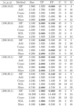
Example 2: The generating scheme is similar as Example 1, except thatf∗(xi) = (2xi1− 1)(2xi2−1), Wij and Ui are independently from N(0,1) andi ∼N(0,1). It is clear that the underlying regression model includes interaction terms, and thus the additive model assumption is no longer valid.
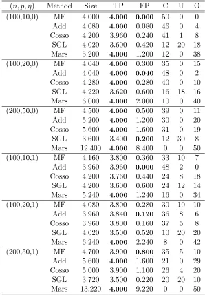
For each example, different scenarios are considered with η = 0 or 1, and (n, p) = (100,10), (100,20) or (200,50). Each scenario is replicated 50 times, and the averaged performance measures are summarized in Tables 1 and 2. Specifically, Size represents the averaged number of selected informative variables, TP represents the number of truly in-formative variables selected, FP represents the number of truly non-inin-formative variables selected and C, U, O are the times of correct-fitting, under-fitting and over-fitting, respec-tively.
It is evident that the proposed MF method delivers superior selection performance against the other three competitors. In Table 1 where the true model is indeed additive, MF performs similarly as Add and SGL, whereas Cosso and Mars appear more likely to overfit. In Table 2 where the true model consists of interaction terms, the performance of MF becomes competitive, but Add tends to under-fit more frequently, and Cosso, Mars and SGL tend to overfit as the dimension increases. Furthermore, in both examples with η= 1, it is clear that the correlation among variables increases the difficulty of selecting the truly informative variables, yet the proposed MF method still outperforms its competitors. Furthermore, it is also noted that the estimation accuracy of MF outperforms SGL, but it is omitted here as only MF and SGL estimate the gradient functiong, whereas Add, Cosso and Mars estimate the regression function f.
4.2 Real examples
(n, p, η) Method Size TP FP C U O (100,10,0) MF 4.000 4.000 0.000 50 0 0
Add 4.080 4.000 0.080 46 0 4 Cosso 4.200 3.960 0.240 41 1 8 SGL 4.020 3.600 0.420 12 20 18 Mars 5.200 4.000 1.200 12 0 38 (100,20,0) MF 4.040 4.000 0.300 35 0 15 Add 4.040 4.000 0.040 48 0 2 Cosso 4.280 4.000 0.280 40 0 10
SGL 4.220 3.620 0.600 16 18 16 Mars 6.000 4.000 2.000 10 0 40 (200,50,0) MF 4.500 4.000 0.500 39 0 11 Add 5.200 4.000 1.200 30 0 20 Cosso 5.600 4.000 1.600 31 0 19 SGL 3.600 3.400 0.200 12 30 8 Mars 12.400 4.000 8.400 0 0 50 (100,10,1) MF 4.160 3.800 0.360 33 10 7
Add 3.960 3.960 0.000 48 2 0 Cosso 4.200 3.760 0.440 24 8 18
SGL 4.200 3.600 0.600 24 12 14 Mars 5.240 4.000 1.240 16 0 34 (100,20,1) MF 4.080 3.800 0.280 30 10 10 Add 3.960 3.840 0.120 36 8 6 Cosso 3.960 3.800 0.160 37 5 8 SGL 4.020 3.500 0.520 10 20 20 Mars 6.240 4.000 2.240 8 0 42 (200,50,1) MF 4.700 3.900 0.800 35 5 10 Add 5.600 4.000 1.600 21 0 29 Cosso 5.000 3.900 1.100 26 4 20 SGL 3.720 3.500 0.220 20 20 10 Mars 13.220 4.000 9.220 0 0 50
Table 1: The averaged performance measures of various variable selection methods in Ex-ample 1.
(n, p, η) Method Size TP FP C U O (100,10,0) MF 1.960 1.920 0.080 43 3 4 Add 2.140 1.760 0.380 25 9 16 Cosso 2.920 1.920 1.000 15 3 32 SGL 2.320 1.920 0.400 30 4 16 Mars 4.000 2.000 2.000 8 0 42 (100,20,0) MF 2.100 2.000 0.100 45 0 5
Add 2.200 1.800 0.400 30 8 12 Cosso 4.320 1.920 2.400 10 3 37 SGL 2.220 2.000 0.220 42 0 8 Mars 4.240 1.920 2.320 14 2 34 (200,50,0) MF 2.100 2.000 0.100 45 0 5
Add 2.920 1.920 1.000 28 2 20 Cosso 2.200 1.800 0.400 25 10 15 SGL 1.800 1.800 0.000 42 8 0 Mars 8.200 2.000 6.200 0 0 50 (100,10,1) MF 2.160 2.000 0.160 42 0 8
Add 2.360 1.560 0.800 16 12 22 Cosso 3.600 2.000 1.600 10 0 40 SGL 2.300 2.000 0.300 35 0 15 Mars 4.240 2.000 2.240 10 0 40 (100,20,1) MF 2.040 1.920 0.120 40 4 6
Add 2.460 1.920 0.540 34 4 12 Cosso 3.240 1.800 1.440 9 10 31 SGL 2.120 1.800 0.320 28 10 12 Mars 6.740 2.000 4.740 0 0 50 (200,50,1) MF 2.160 1.960 0.200 40 2 8
Add 16.200 1.800 14.400 17 9 24 Cosso 2.340 1.800 0.540 28 10 22 SGL 2.460 1.960 0.500 23 2 25 Mars 8.160 1.960 6.240 0 2 48
Table 2: The averaged performance measures of various variable selection methods in Ex-ample 2.
digit recognition data. Each example is replicated 100 times, and the averaged prediction errors by MF, Add, Cosso and Mars are summarized in Tables 3-5.
Variables MF Add Cosso SGL Mars
CRIM - √ √ - √
ZN - - - -
-INDUS - - - -
-CHAS - - - -
-NOX - √ - - √
RM √ √ √ √ √
AGE - - - -
-DIS - √ - - √
RAD - - - - √
TAX - √ - -
-PTRATIO - √ - - √
B - - - - √
LSTAT √ √ √ √ √
Pred. Err. 1.774(0.0931) 1.780(0.0916) 1.797(0.0924) 1.774(0.0931) 1.956(0.0939)
Table 3: The selected variables as well as the corresponding prediction errors by various selection methods in the Boston housing dataset.
Variables MF Add Cosso SGL Mars
M √ √ √ √ √
DM - - - -
-DW - - - -
-VDHT - √ - √ √
WDSP - - - - √
HMDT √ - √ √ √
SBTH √ √ √ √ √
IBHT - √ - √ √
DGPG - √ - - √
IBTP √ - √ √ √
VSTY - √ - √ √
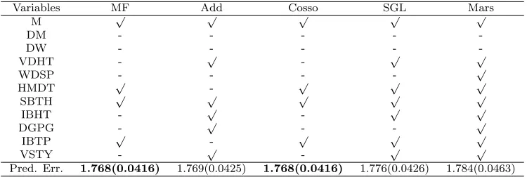
Pred. Err. 1.768(0.0416) 1.769(0.0425) 1.768(0.0416) 1.776(0.0426) 1.784(0.0463)
Table 4: The selected variables as well as the corresponding prediction errors by various selection methods in the Ozone concentration dataset.
MF Add Cosso SGL Mars
No. of variables 2 48 8 4 18
Prediction error 1.857(0.0316) 1.871(0.0310) 1.878(0.0314) 1.875(0.0324) 1.879(0.0310) Table 5: The number of selected variables and the prediction errors by various selection
methods in the digit recognition dataset.
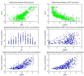
select four variables but Add and Mars select more. One discrepancy is the variable IBTP, which is selected by MF, Cosso, SGL and Mars but not by Add. As claimed in Gregory et al. (2012), M, SBTH and IBTP are three most important meteorological variables related to Ozone concentration as all of them describe the temperature changes. Meanwhile, MF and Cosso show smaller prediction error than SGL and Mars, which implies that SGL and Mars may include some non-informative variables. Figure 1 displays scatter plots of the responses against the selected variables by MF in the Boston housing data and the Ozone concentration data. It is clear that all the selected variables show moderate to strong re-lationship with the responses. For digit recognition data, MF selects much less variables than the other competitors and provides smaller prediction error. Figure 2 shows some randomly selected digits of 3 and 5 and the two selected informative variables, where the left informative variable is always contained in digit 5 and the right one is always contained in digit 3.
Figure 2: Some randomly selected digit 3, digit 5 and the two selected informative variables.
5. Summary
This article proposes a model-free variable selection method, which is in sharp contrast to most existing methods relying on various model assumptions. The proposed method makes use of the natural connection between informative variables and sparse gradients, and formulates the variable selection task in a flexible framework of learning gradients. Additionally, we introduce a coefficient-based representation to facilitate variable selection in the learning framework. A block-wise coordinate decent algorithm is developed to make efficient computation for large-scale problems feasible. More importantly, we establish the estimation and variable selection consistencies of the proposed method without assuming any restrictive model assumption. The effectiveness of the proposed method is also sup-ported by numerical experiments on simulated and real examples. It is worth pointing out that the computational cost of the proposed method can be expensive, as it allows for a more flexible modeling framework in RKHS. The extension of the proposed method to diverging dimension is also challenging as a model-free framework with diverging dimension can be too flexible to analyze. One possible remedy is to pre-screen the non-informative variables via some model-free screening methods (Li et al., 2012) to shrink the size of candidate variables.
Acknowledgments
Appendix A. technical proofs
Proof of Lemma 1: First, note that under Assumption A1 and A2, the probability densityp(x) is bounded, and thus there exists some constantc7such that supx∈Xp(x)≤c7. Moreover, denoteXt={x∈ X :dX(x, ∂X)< t}, then we haveρX(Xt)≤c8tfor anytgiven a constant c8, where ∂X is the boundary of the compact support X, ρX is the marginal distribution anddX(x, ∂X) = infu∈∂XdX(x,u).
Since g0 is the minimizer ofE(g), the functional derivative ofE(g) at g0 yields that for any arbitrary function vector δ(x),
Z
X
Z
X
w(x,u) f(x)−f(u) +g0(x)T(u−x)
(u−x)Tδ(x)dρX(u)dρX(x) =0p,
where 0p is a p-dimensional vector with all zeros. As the above equality is true for any δ(x), it implies that for any given x,
Z
X
w(x,u) f(x)−f(u) +g0(x)T(u−x)
(u−x)dρX(u) =0p.
For simplicity, denote M(x) = R
Xw(x,u)(u−x)(u−x)TdρX(u) a function matrix, and d(x) =RX w(x,u)(u−x) (f(u)−f(x))dρX(u) a function vector. ThenM(x)g0(x)− d(x) = 0 for any given x. Let Xτ = {x : dX(x, ∂X) ≥ τn, p(x) ≥ c2τnθ +τ
1/2
n }, then by Assumption A2,
P(Xτc)≤P(dX(x, ∂X)< τn) +P
p(x)< c2τnθ+τn1/2
≤c8τn+ (c2τnθ+τn1/2)|X |, where|X | denotes the Lebesgue measure ofX. For anyx∈ Xτ,
M(x) = Z
w(x,u)(u−x)(u−x)Tp(u)du
≥ τn1/2 Z
dX(x,u)<τn
e−
kx−uk22
2τn2 (u−x)(u−x)Tdu=τp+5/2
n Z
ktk2<1 e−
ktk22
2 t tTdt,
where t = (u−x)/τn. The inequality follows from Assumption A2 and the fact that p(u) ≥ p(x) − |p(u) −p(x)| ≥ p(x)−c2d(x,u)θ ≥ τn1/2 on Xτ. As the support X is non-degenerate by assumption A1, R
ktk2<1e
−ktk22
2 t tTdt is always positive definite. So its smallest eigenvalue, denoted asφmin, is positive, and thus the smallest eigenvalue ofM(x) must be larger thanφminτnp+5/2, which is also positive.
As M(x) is invertible for anyx∈ Xτ, we haveg0(x) =
M(x)−1d(x), and thus
kg0(x)−g∗(x)k
2≤ k(M(x))−1k2kd(x)−M(x)g∗(x)k2. Furthermore,
kd(x)−M(x)g∗(x)k
2 = Z
X
w(x,u)(u−x) f(u)−f(x)−g∗(x)T(u−x)
dρX(u)
≤
Z
w(x,u)(u−x) f(u)−f(x)−g
∗(x)T(u−x)
p(u)du
≤ c1c8 Z
w(x,u)ku−xk23du≤c1c8τnp+3 Z
e−
ktk2
2 2 ktk3
Therefore, for any x∈ Xτ,
kg0(x)−g∗(x)k
2 ≤ kM(x)−1k2kd(x)−M(x)g∗(x)k2≤
c1c8τn1/2 φmin
Z e−
ktk22
2 ktk3 2dt, which converges to 0 for any x ∈ Xτ. Since P(x∈ Xτ) → 1 as τn → 0, the desired result follows immediately.
Next, as E(g)−2σ2s > 0 for any g, we have 0 ≤ E(g0)−2σ2
s ≤ E(g∗) −2σs2. By Proposition 3 in Ye and Xie (2012), E(g∗)−2σ2
s ≤ O(τ p+4
n ) → 0 as τn → 0. Therefore,
E(g0)−2σ2
s →0 as τn→0.
To proceed further, we note that the proof of Theorem 2 is substantially different from conventional error analysis as in Mukerjee and Zhou (2006) and Ye and Xie (2012). In our setting, we consider the coefficient-based spaceHz={g: g(x) =Pn
i=1aiK(xi,x), ai∈ R} as the candidate functional space, which depends on{xi}ni=1. One difficulty arises is thatg∗ may not be contained inHpzand thusJ(g∗) can not be defined. To circumvent this difficulty,
we introduce an intermediate learning algorithm as a bridge for the error analysis, so that standard empirical process and approximation theories can be used.
Define a vector-valued functional space as HKp = {g = (g1, ..., gp)T, gj ∈ HK}, and
Hpz = {g = (g1, ..., gp)T, gj ∈ Hz}. Furthermore, denote the empirical error used in our
algorithm as
Ez(g) =
1 n(n−1)
n X
i,j=1 ωij
yj−yi−g(xi)T(xj−xi) 2
.
Clearly,E(Ez(g)) =E(g) for any g∈ HpK.
In order to establish the consistency results, we introduce an intermediate learning algorithm,
¯
g= argmin
g∈HpK
1 n(n−1)
n X
i,j=1 wij
yi−yj −g(xi)(xi−xj) 2
+ρn p X
l=1
πlkglk2K, (9)
whereρn=n−η withη= 4(p1+2). Note that (9) is a weighted version of the original gradient learning in Mukherjee and Zhou (2006). By the representor theorem, each element of ¯g in (9) has a closed solution with the form
¯ gl= n X t=1 ¯
αltK(x,xt), for l= 1, ..., p.
Denote ¯αl= ( ¯αl1, ...,α¯ln)T satisfies the linear system ρnπlKα¯l+
1 n(n−1)
n X
i,j=1 ωij
yj −yi−g¯(xi)T(xj−xi)
(K)Ti [xj−xi]l = 0, (10)
where (K)i represents the i-th row ofK. Without loss of generality, we assume that K is invertible. In this case, we can solve for ¯αlt as follows:
ρnπlα¯lt=− 1
n(n−1) n X
j=1 ωtj
yj−yt−g¯(xt)T(xj−xt)
With these preparations, we are now in the position to decompose the excess error as follows.
Proposition 4 Let ϕ0(z) =Ez(g∗)− E(g∗) and ϕ1(z) =E(ˆg)− Ez(ˆg). Then the following
inequality holds for any 0< ε≤1,
E(ˆg) +λn p X
l=1
πlJ(ˆgl)≤ϕ1(z) + 2ϕ0(z) + Λn(ε, ρ, K),
where
Λn(ε, ρ, K) = (1 +ε)E(g∗) + p0 X
l=1
ρnπl(kgl∗k2K− k¯glk2K) +c2n/ε, (12)
withcn= ρcxpλn
n
√
n−1 and cx≥supxkxk. In the literature of statistical learning theory,ϕ0(z), ϕ1(z) are called the sample error and Λ(λn) is the approximation error.
Proof of Proposition 4: First of all, by the H¨older inequality, it follows from 11 that:
J(¯gl)≤
cx ρnπl
√
n−1 p
Ez(¯g), l= 1, ..., p. (13)
The above inequality in connection with the definition of ˆg yields that
E(ˆg) +λn p X
l=1
πlJ(ˆgl) = E(ˆg)− Ez(ˆg) +Ez(ˆg) +λn p X
l=1
πlJ(ˆgl)
≤ E(ˆg)− Ez(ˆg) +Ez(¯g) +λn
p X
l=1
πlJ(¯gl)
≤ E(ˆg)− Ez(ˆg) +Ez(¯g) +
cxλn
√
n−1 p X
l=1 1 ρn
p
Ez(¯g)
≤ E(ˆg)− Ez(ˆg) + (1 +ε)Ez(¯g) +c2n/ε
≤ E(ˆg)− Ez(ˆg) + (1 +ε)Ez(g∗) + 2
p X
l=1
ρnπl(kgl∗k2K− k¯glk2K) +c2n/ε
≤ E(ˆg)− Ez(ˆg) + (1 +ε)Ez(g∗) + 2
p0 X
l=1
ρnπl(kgl∗k2K− k¯glk2K) +c2n/ε,
where the first inequality follows from the definition of ˆg, the second inequality is derived based on 13, the third inequality follows from the fact √xy ≤ εx+2y/ε for any ε > 0, the fourth inequality follows from the definition of ¯g, and the last inequality is due to the
assumption thatg∗l = 0 for any l > p0.
Next, For any given value R >0, define the functional subspace with bounded J(g) as
and
S(R,λn) = sup
g∈Hp R
|E(g)− Ez(g)|.
Then the quantityS(R, λn) can be bounded using the McDiarmid’s inequality (McDiarmid, 1989).
Lemma 5 (McDiarmid’s Inequality) LetZ1, ..., Znbe independent random variables taking
values in a set Z, and assume thatf :Zn→
Rsatisfies
sup z1,...,zn,z0i∈Z
|f(z1, ..., zn)−f(z1, ..., zi0, ..., zn)| ≤Ci,
for everyi∈ {1,2, ..., n}. Then, for every t >0,
P{|f(z1, ..., zn)−E(f(z1, ..., zn))| ≥t} ≤2 exp
− 2t
2 Pn
i=1Ci2
.
This result implies that, as soon as one has a function of nindependent random variables, whose variation is bounded when only one variable is modified, the function will satisfy a Hoeffding-type inequality.
Lemma 6 If |y| ≤ Mn and Assumptions A1-A3 hold, then for any constant R > 0 and ε >0 , there holds
P(|S(R, λn)−E(S(R, λn))| ≥ε)≤2 exp − nε
2 8(Mn+cxnψ/2R
c4λn )
4 !
.
In addition, there exists a constantc5, such that
P(|Ez(g∗)− E(g∗)| ≥ε)≤2 exp −
nε2 8(Mn+cxPp
l=1kgl∗kK) 4
!
. (14)
Proof of Lemma 6: It suffices to verify the conditions required by the McDiarmid’s inequality. For this purpose, we define (x0, y0) as a sample point drawn from the distribution ρ(x, y) and independent of (xi, yi). Denote by z0 the modified training sample which is the same as z except that thei-th observation (xi, yi) is replaced with (x0, y0). Let h(zi,zj) = ωij(yj−yi−g(xi)T(xj−xi))2 with any fixedg∈ HpR, then we decomposeEz(g) as follows,
Ez(g) =
1 n(n−1)
n X
k6=i,j6=i
h(zk,zj) + 1 n(n−1)
n X
j=1
h(zi,zj) + 1 n(n−1)
n X
k=1
h(zk,zi).
Note that if z is replaced by z0, the difference between Ez(g) and Ez0(g) boils down to
the differences between the second and third components of the above decomposition. By Assumption A3, we see thatπl > c4 for any l. Then it follows that
Ez(g)−Ez0(g)≤
4(Mn+cxPpl=1kglkK)2
n ≤
4(Mn+cxnψ/2Plp=1kα(l)k2)2
n ≤
4(Mn+cxn
ψ/2R c4λn )
2
where the second inequality follows from the H¨older inequality and Assumption A1. Inter-changing the roles of z andz0 yields that
|Ez(g)− Ez0(g)| ≤
4(Mn+cxnψ/2R
c4λn )
2
n , ∀g∈ H
p R.
Then applying the McDiarmid’s inequality, we have
P(|S(R,λn)−E(S(R, λn))| ≥ε)≤2 exp −
nε2 8(Mn+cxn
ψ/2R c4λn )
4 !
.
In contrast with the first one, it is easier to obtain the second result in Lemma 6, since it only involves the fixed function g∗. As a similar argument to the first one, we can set
Ci = 4(Mn+cx Pp
l=1kg
∗ lkK)2
n . Thus plugging Ci into the McDiarmid’s inequality, our desired
result follows immediately.
Proposition 7 Assume the assumptions of Theorem 2 are met. IfEz(0) = n(n1−1)Pn
i,j=1(yi− yj)2 is upper bounded by M0, then there exists a constant c9 such that for any δ ∈ (0,1),
with probability at least 1−δ,
J(ˆg)≤c9 p
log(4/δ)
Mn2n−1/2+n2ψ−21M2 0λ
−2
n +ετnp+ max l≤p0
ρnπlkg∗l −gl¯kK+c2n/ε
where cn is defined as Proposition 4. In addition, there holds
E(ˆg)−2σs2≤c9 p
log(4/δ)
Mn2n−1/2+n2ψ−2 1λ−2
n +ετnp+ max l≤p0
ρnπlkgl∗−gl¯kK+c2n/ε
Proof of Proposition 7: By Lemma 2 of Ye and Xie (2012), we have
E(S(R, λn))≤
(Mn+cxnψ/2R
c4λn )
2
√
n ,
which, together with Lemma 6, implies that with probability at least 1−δ,
ϕ1(z)≤ |S(R, λn)| ≤3 r
log(2/δ) n
Mn+
cxnψ/2R c4λn
2
. (15)
By Proposition 4, we recall that
J(ˆg) +E(ˆg)≤ϕ1(z) + 2ϕ0(z) + Λn(ε, ρ, K), where Λn(ε, ρ, K) = (1 +ε)E(g∗) +Pp0
l=1ρnπl(kg
∗
lk2K− kgl¯k2K) +c2n/ε. In addition, note that the Hessian matrixH∗(x) of f∗ is bounded uniformly on x, it is easy to verify that
E(g∗)−2σ2
s =O(τn4+p), which implies that
Λn(ε, ρ, K)−2σ2s ≤O(ετnp+ max l≤p0
sinceσs2 =O(τnp) by definition.
Thus, combining 14 in Lemma 6, 15 with 16 , for some constantc9, we have J(ˆg) +E(ˆg)−2σ2s
≤ c9 p
log(4/δ)
Mn2n−1/2+n2ψ−2 1R2λ−2
n +ετnp+ max l≤p0
ρnπlkg∗l −¯glkK+c2n/ε
with probability at least 1−δ. Finally, we give an explicit bound for R. Following the definition of ˆg, we have
Ez(ˆg) +J(ˆg)≤ Ez(0) +J(0)≤M0, which implies ˆg ∈ HpM
0, and thus R = M0. As a consequence, the first and the second desired inequalities follow immediately after the fact thatE(ˆg)−2σ2s ≥0 andJ(ˆg)≥0. Proof of Theorem 2: For given constant c6>0,C is denoted to be the following event,
C=
n ˆ
g :E(ˆg)−2σ2s > c6 p
log(4/δ)
n−1/4+n2ψ−2 1λ−2
n +ετnp+n
− 1
2(p+2)+n−(1− 1 2(p+2))λ2
n/ε
. o
.
Then, we split C into three different events as follows,
P(C) = PC ∩ {|y| ≤n1/8, U ≤M0}c
+PC ∩ {|y| ≤n1/8, U ≤M0}
≤ P(|y|> n1/8) +P(|y| ≤n1/8, U > M0) +P
C ∩ {|y| ≤n1/8, U ≤M0}
,
where U = n(n1−1)Pn
i,j=1(yi−yj)2 and M0 = 4B2 + 2σ2 + 1 with B an upper bound of f∗(x). The existence ofB is due to the assumptions thatx has a compact support andf∗ is continuous Now we bound these three probabilities one by one.
First, by Chebyshev inequality, P(|y| > n81) = E(P(f∗(x) + > n 1
8|x)) ≤ O(n− 1 4), where the last inequality is due to boundedf∗(x). For the second probability, note thatU is a U-statistic with meanE(U) =E(E(U|xi,xj)) =E(f∗(xi)−f∗(x0))2+2σ2 ≤4B2+2σ2. By Bernstein’s inequality for U-statistic (Janson, 2004),
P(|y| ≤n1/8, U > M0)≤P(U > E(U) + 1||y| ≤n1/8)≤exp
− 1
16n 3/4
,
where (yi−yj)2 is upper bounded by 4n1/4, which completes the second term.
Now we turn to the third term. Within the set {|y| ≤n1/8, U ≤M0}, by Proposition 7,
E(ˆg)−2σs2≤c9 p
log(4/δ)n−1/4+n2ψ−2 1M2
0λ−n2+ετnp+ max l≤p0
ρnπlkgl∗−¯glkK+c2n/ε
.
With the choice of ρl = n−η with η = 4(p1+2) for all l, we have kgl∗−¯glkK = O(n
− 1 4(p+2))
according to theorems 14, 17, 19 in Mukherjee and Zhou (2006). In addition,cn= ρcxpλn
n
√
n−1 = O(n−(12−η)λn). Thus with probability at least 1−δ, for some constantc6,
E(ˆg)−2σs2≤c6 p
log(4/δ)
n−1/4+n2ψ−2 1λ−2
n +ετnp+n
− 1
2(p+2) +n−(1− 1 2(p+2))λ2
n/ε
Specifically, with λn=n 2ψ−1
4 + 1 4(p+2),τ
n=n
− θ
4p(p+2)(p+4+3θ) and ε=τ4
n, we have
E(ˆg)−2σs2 ≤c6 p
log(4/δ)n−Θ,
where Θ = minn4p(p+2)(θ(p+4)p+4+3θ),2(p1+2),2pp2(p(p+2)(+4+3p+4+3θ)−2θθ)o. Proof of Theorem 3: First, we show that kαˆ(l)k2 = 0 for any l > p0 by contradiction. Suppose thatkαˆ(l)k2>0 for somel > p0. Taking the first derivative of (4) with respect to α(l) yields that
2 n(n−1)
n X
i,j=1
wij(yi−yj−gˆ(xi)T(xi−xj))(xil−xjl)Kl=−
λnπlαˆ(l)
kαˆ(l)k2 . (17)
Note that the norm of the right-hand side divided byn1/2 isn−1/2λ
nπl, which diverges to
∞ by Assumption A3. Then the contradiction can be concluded by showing the norm of the left-hand side is smaller than O(n1/2).
For simplicity, denote Bz(g) = n(n2−1)Pn
i,j=1wij(yi −yj −g(xi)T(xi −xj)). As the elements in both x and Kl are bounded by Assumption A1, it suffices to show |Bz(ˆg)| is
bounded. DenoteC = n
ˆ
g:|Bz(ˆg)|> c10 p
log(4/δ)(n−Θ/2+nψ−21λ−1
n +n−3/8) o
. As in the proof of Theorem 2, we decomposeP(C) as
P(C) = PC ∩ {|y| ≤n1/8, U ≤M0}c
+PC ∩ {|y| ≤n1/8, U ≤M0}
≤ P(|y|> n1/8) +P(|y| ≤n1/8, U > M0) +P
C ∩ {|y| ≤n1/8, U ≤M0}
.
whereU and M0 are the same as in Theorem 2.
Following the proof of Theorem 2, the first two probabilities can be bounded asP(|y|> n1/8) ≤ O(n−1/4) and P(|y| ≤ n1/8, U > M0) ≤ exp
−1 16n
3/4 . To bound the third probability, a slight modification of the proof of Proposition 7 yields that when |y| ≤n1/8 and U ≤M0, we haveJ(ˆg)≤M0 and with probability at least 1−δ/2,
|Bz(ˆg)−E(Bz(ˆg)| ≤3
r
log(4/δ) n
n1/8+cxn ψ/2M
0 c4λn
.
We then bound |E(Bz(ˆg)|as follows,
|E(Bz(ˆg))| =
Z X Z X
w(x,u)f∗(x)−f∗(u) + ˆg(x)T(u−x)dρX(x)dρX(u) ≤ Z X Z X
w(x,u)
f∗(x)−f∗(u) + ˆg(x)T(u−x)
2
dρX(x)dρX(u) 1/2
≤
Z
X
Z
X
w(x,u)
f∗(x)−f∗(u) + ˆg(x)T(u−x)2dρX(x)dρX(u)1/2 =
E(ˆg)−2σ2s1/2.
we have with probability at least 1−δ/2 that
|Bz(ˆg)| ≤c10 p
log(4/δ)(n−Θ/2+nψ−21λ−1
n +n−3/8). (18) This implies that P(C)≤δ/2 +O(n−1/4) for any given δ. Then it is clear that the norm of the left-hand side of (17) divided byn1/2 will converge to 0 in probability, which contradicts with the fact that the norm of the right-hand side divided byn1/2diverges to∞. Therefore, we have kαˆ(l)k2 = 0 for any l > p0.
Next, we show thatkαˆ(l)k2 >0 for anyl≤p0. Let ¯Xτ ={x∈ X :d(x, ∂X)> τn, p(x)> τn+c2τnθ}. Same as the proof of Theorem 5 in Ye and Xie (2012), for some given constant c11, we have
Z
¯
Xτ
kˆg(x)−g∗(x)k2
2dρX(x)≤c11τn−(p+3)
τnp+4+E(ˆg)−2σs2. According to Theorem 2, it can be showed that
Z
¯
Xτ
kgˆ(x)−g∗(x)k22dρX(x)→0.
Now suppose kαˆ(l)k2 = 0 for some l≤p0, which implies Z
¯
Xτ
kgˆ(x)−g∗(x)k2
2dρX(x) = Z
¯
Xτ
kgl∗(x)k22dρX(x).
As τn → 0, R
¯
Xτkg
∗
l(x)k22dρX(x) ≥ R
X \Xtkg
∗
l(x)k22dρX(x), which is a positive constant by Assumption A4, and then leads to the contradiction. Combining the above two statements implies the desired variable selection consistency.
References
H., Bondell and L., Li. Shrinkage inverse regression estimation for model free variable selection.Journal of the Royal Statistical Society, Series B., 71: 287-299, 2009.
K. Brabanter, J. Brabanter and B. Moor. Derivative estimation with local polynomial fit-ting. Journal of Machine Learning Research, 14: 281-301, 2014.
L. Breiman. Better subset regresson using nonnegative garrote.Technometrics, 37: 373-384, 1995.
L. Breiman and J. Friedman. Estimating optimal transformations for multiple regression and correlation. Journal of the American Statistical Association, 80: 580-598, 1985.
C. Cortes and V. Vapnik. Support vector networks.Journal of Machine Learning Research, 20: 273-297, 1995.
J. Fan, F. Yang and R. Song. Nonparametric independence screening in sparse ultrahigh dimensional additive models. Journal of the American Statistical Association, 106: 544-557, 2011.
J. Friedman. Multivariate Adaptive Regression Splines. The Annal of Statistics, 19: 1-67, 1991.
E. Gregory, J. Fred and W. Henryk. On dimension-independent rates of convergence for function approximation with Gaussian Kernels. SIAM Journal on Numerical Analysis, 50: 247-271, 2012.
R. Genuer, J. Poggi and C. Tuleau-Malot. Variable selection using random forests.Pattern Recognition Letters, 31: 2225-2236, 2010.
N. Hao and H. Zhang. Interaction screening for ultrahigh-dimensional data.Journal of the American Statistical Association, 109: 1285-1301, 2014.
W. H¨ardle and T. Gasser. On robust kernel estimation of derivatives of regression functions.
Scandinavian Journal of Statistics, 12: 233-240, 1985.
J. L. Horowitz and E. Mammen. Rate-optimal estimation for a general class of nonparamet-ric regression models with unknown link functions. Annal of Statistics, 35: 2589-2619, 2007.
J. Huang, J. Horowitz and F. Wei. Variable selection in nonparameteric additive models.
The Annals of Statistics, 38: 2282-2313, 2010.
J. Huang, and L. Yang. Identification of non-linear additive autoregressive models.Journal of the Royal Statistical Society: Series B, 66: 463-477, 2004.
S. Janson. Large deviations for sums of partly dependent random variables.Random Struc-tures and Algorithms, 24: 234-248, 2004.
R. Jarrow, D. Ruppert and Y. Yu. Estimating the term structure of corporate debt with a semiparametric penalized spline model. Journal of the American Statistical Association, 99: 57-66, 2004.
L. Li, D. Cook and C. Nachtsheim. Model-free variable selection. Journal of the Royal Statistical Society, Series B., 67: 285-299, 2005.
R. Li, W. Zhong and L. Zhu. Feature screening via distance correlation learning. Journal of the American Statistical Association, 107: 1129-1139, 2012.
Y. Lin. A note on margin-based loss functions in classification. Statistics and Probability Letters, 68: 73-82, 2004.
Y. Lin and H. Zhang. Component selection and smoothing in multivariate non-parametric regression. Annal of Statistics, 34: 2272-2297, 2006.
Y. Liu and Y. Wu. Variable selection via a combination of the L0 and L1 penalties.Journal of Computational and Graphical Statistics, 16: 782-798, 2007.
C. McDiarmid,. On the method of bounded differences.In Surveys in Combinatorics, 141: 148-188.
S. Mukherjee and D. Zhou. Learning coordinate covariates via gradient.Journal of Machine Learning Research, 7: 519-549, 2006.
B. Scholk¨opf and A.J. Smola. Learning with kernels: Support vector machines, regulariza-tion, optimizaregulariza-tion, and beyond. MIT Press, 2002.
X. Shen, W. Pan and Y. Zhu. Likelihood-based selection and sharp parameter estimation.
Journal of the American Statistical Association, 107: 223-232, 2012.
T. Shively, R. Kohn and S. Wood. Variable selection and function estimation in additive non-parametric regression using a data-based prior. Journal of the American Statistical Association, 94: 777-794, 1999.
L. Stefanski, Y. Wu and K. White. Variable selection in nonparametric classification via measurement error model selection likelihoods.Journal of the American Statistical Asso-ciation, 109: 574-589, 2014.
W. Sun, J. Wang and Y. Fang. Consistent selection of tuning parameters via variable selection stability. Journal of Machine Learning Research, 14: 3419-3440, 2013.
R. Tibshirani. Regression shrinkage and selection via the LASSO. Journal of the Royal Statistical Society: Series B, 58: 267-288, 1996.
G. Wahba. Support vector machines, reproducing kernel hilbert spaces, and randomized GACV. Advances in kernel methods, 69-88, 1999.
L. Xue. Consistent variable selection in additive models. Statistica Sinica, 19: 1281-1296, 2009.
Y. Yang and H. Zou. A fast unified algorithm for solving group-lasso penalized learning problems. Statistics and Computing, 25: 1129-1141, 2015
G. Ye and X. Xie. Learning sparse gradients for variable selection and dimension reduction.
Journal of Machine Learning Research, 87: 303-355, 2012.
M. Yuan and Y. Lin. Model selection and estimation in regression with group variables.
Journal of the Royal Statistical Society: Series B, 68: 49-67, 2006
L. Zhu, L. Li, R. Li and L. Zhu. Model-free feature screening for ultra-high dimensional data. Journal of the American Statistical Association, 106: 1464-1475, 2011.