Distributed Coordinate Descent Method for Learning with Big Data
Peter Richt´arik [email protected]
School of Mathematics University of Edinburgh
6317 James Clerk Maxwell Building Peter Guthrie Tait Road
Edinburgh, EH9 3FD
Martin Tak´aˇc [email protected]
Industrial and Systems Engineering Department Lehigh University
H.S. Mohler Laboratory 200 West Packer Avenue Bethlehem, PA 18015, USA
Editor:Koby Crammer
Abstract
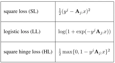
In this paper we develop and analyze Hydra: HYbriD cooRdinAte descent method for solving loss minimization problems with big data. We initially partition the coordinates (features) and assign each partition to a different node of a cluster. At every iteration, each node picks a random subset of the coordinates from those it owns, independently from the other computers, and in parallel computes and applies updates to the selected coordinates based on a simple closed-form formula. We give bounds on the number of iterations sufficient to approximately solve the problem with high probability, and show how it depends on the data and on the partitioning. We perform numerical experiments with a LASSO instance described by a 3TB matrix.
Keywords: stochastic methods, parallel coordinate descent, distributed algorithms, boosting
1. Introduction
Randomized coordinate descent methods (CDMs) are increasingly popular in many learning tasks, including boosting, large scale regression and training linear support vector machines. CDMs up-date a single randomly chosen coordinate at a time by moving in the direction of the negative partial derivative (for smooth losses). Methods of this type, in various settings, were studied by several authors, including Hsieh et al. (2008); Shalev-Shwartz and Tewari (2009); Nesterov (2012); Richt´arik and Tak´aˇc (2014); Necoara et al. (2012); Tappenden et al. (2013); Shalev-Shwartz and Zhang (2013b); Lu and Xiao (2015).
theory was developed for methods that update a random subset of blocks of coordinates at a time Richt´arik and Tak´aˇc (2015); Fercoq and Richt´arik (2013). Further recent works on parallel coordi-nate descent include (Richt´arik and Tak´aˇc, 2012; Mukherjee et al., 2013; Fercoq, 2013; Tappenden et al., 2015; Shalev-Shwartz and Zhang, 2013a).
However, none of these methods are directly scalable to problems of sizes so large that a single computer is unable to store the data describing the instance, or is unable to do so efficiently (e.g., in memory). In a big data scenario of this type, it is imperative to split the data across several nodes (computers) of a cluster, and design efficient methods for this memory-distributed setting.
Hydra. In this work we design and analyze the first distributed coordinate descent method: Hydra: HYbriD cooRdinAte descent. The method is “hybrid” in the sense that it uses parallelism at two levels: i) across a number of nodes in a cluster and ii) utilizing the parallel processing power of individual nodes1.
Assume we havecnodes (computers) available, each with parallel processing power. In Hydra, we initially partition the coordinates {1,2, . . . , d}into c sets, P1, . . . ,Pc, and assign each set to a single computer. For simplicity, we assume that the partition is balanced: |Pk| = |Pl| for all
k, l. Each computerownsthe coordinates belonging to its partition for the duration of the iterative process. Also, these coordinates are stored locally. The data matrix describing the problem is partitioned in such a way that all data describing features belonging toPlis stored at computer l. Now, at each iteration, each computer, independently from the others, chooses a random subset of
τ coordinates from those they own, and computes and applies updates to these coordinates. Hence, once all computers are done,cτ coordinates will have been updated. The resulting vector, stored as
cvectors of sizes=d/ceach, in a distributed way, is the new iterate. This process is repeated until convergence. It is important that the computations are done locally on each node, with minimum communication overhead. We comment on this and further details in the text.
The main insight. We show that the parallelization potential of Hydra, that is, its ability to accelerate asτ is increased, depends on two data-dependent quantities: i) thespectral norm of the data (σ) and ii) apartition-induced norm of the data (σ0). The first quantity completely describes the behavior of the method in thec= 1case. Ifσ is small, then utilization of more processors (i.e., increasingτ) leads to nearly linear speedup. Ifσis large, speedup may be negligible, or there may be no speedup whatsoever. Hence, the size ofσsuggests whether it is worth to use more processors or not. The second quantity, σ0, characterizes the effect of the initial partition on the algorithm, and as such is relevant in the c > 1case. Partitions with small σ0 are preferable. We show that, surprisingly, that as long asτ ≥2, the effect of a bad partitioning is that it most doubles the number of iterations of Hydra. Hence, data partitioning can be used to optimize for different aspects of the method, such as reducing communication complexity, if needed.
For all of these quantities we derive easily computable and interpretable estimates (ωforσand
ω0forσ0), which may be used by practitioners to gauge, a-priori, whether their problem of interest is likely to be a good fit for Hydra or not. We show that for strongly convex losses, Hydra outputs an-accurate solution with probability at least1−ρafter
dβ cτ µlog
1
ρ
iterations (we ignore some small details here), where a single iteration corresponds to changing of
τ coordinates by each of thecnodes;βis a stepsize parameter andµis a strong convexity constant.
square loss (SL) 12(yj−Aj:x)2
logistic loss (LL) log(1 + exp(−yjAj:x))
square hinge loss (HL) 12max{0,1−yjAj:x}2
Table 1: Examples of loss functions`covered by our analysis.
Outline.In Section 2 we describe the structure of the optimization problem we consider in this paper and state assumptions. We then proceed to Section 3, in which we describe the method. In Section 4 we prove bounds on the number of iterations sufficient for Hydra to find an approximate solution with arbitrarily high probability. A discussion of various aspects of our results, as well as a comparison with existing work, can be found in Section 5. Implementation details of our distributed communication protocol are laid out in Section 6. Finally, we comment on our computational experiments with a big data (3TB matrix) L1 regularized least-squares instance in Section 7.
2. The Problem
We study the problem of minimizing regularized loss,
min
x∈RdL(x) :=f(x) +R(x), (1)
wheref is a smooth convex loss, andRis a convex (and possibly nonsmooth) regularizer.
2.1 Loss Functionf
We assume that there exists a positive definite matrixM∈Rd×dsuch that for allx, h∈Rd,
f(x+h)≤f(x) + (f0(x))Th+12hTMh, (2)
and writeM=ATA, whereAis somen-by-dmatrix.
Example. These assumptions are natural satisfied in many popular problems. A typical loss function has the form
f(x) = n X
j=1
`(x,Aj:, yj), (3)
whereA ∈ Rn×dis a matrix encodingnexamples withdfeatures,Aj
:denotesj-th row ofA,`
2.2 RegularizerR
We assume thatRis separable, i.e., that it can be decomposed asR(x) =Pd
i=1Ri(xi), wherexi is thei-th coordinate ofx, and the functionsRi:R→R∪ {+∞}are convex and closed.
Example. The choiceRi(t) = 0fort ∈[0,1]andRi(t) = +∞, otherwise, effectively models bound constraints, which are relevant for SVM dual. Other popular choices areR(x) = λkxk1
(L1-regularizer) andR(x) = λ2kxk2
2(L2-regularizer).
3. Distributed Coordinate Descent
We consider a setup with ccomputers (nods) and first partition the dcoordinates (features) into
csetsP1, . . . ,Pc of equal cardinality,s := d/c, and assign set Pl to nodel. Hydra is described in Algorithm 1. Hydra’s convergence rate depends on the partition; we comment on this later in Sections 4 and 5. Here we simply assume that we work with a fixed partition. We now comment on the steps.
Algorithm 1:Hydra: HYbriD cooRdinAte descent 1 Parameters:x0 ∈Rd;{P1, . . . ,Pc};β >0,τ;k←0;
2 repeat
3 xk+1←xk;
4 for each computerl∈ {1, . . . , c}in parallel do 5 Pick a random set of coordinatesSˆl⊆ Pl,|Sˆl|=τ
6 for each i∈Sˆlin parallel do
7 hik←arg mintfi0(xk)t+Miiβ2 t2+Ri(xik+t); 8 Apply the update:xik+1 ←xik+1+hik;
9 until happy;
Step 3. Here we are just establishing a way of labeling the iterates. Starting withxk, all c computers modify cτ entries of xk in total, in a distributed way, and the result is called xk+1.
No computer is allowed to proceed before all computers are done with computing their updates. The resulting vector, xk+1, is the new iterate. Note that, due to this, our method is inherently
synchronous.In practice, a carefully designed asynchronous implementation will be faster, and our experiments in Section 7 are done with such an implementation.
Steps 4–5.At every iteration, each of theccomputers picks a random subset ofτfeatures from those that it owns, uniformly at random, independently of the choice of the other computers. LetSˆl denote the set picked by nodel. More formally, we require that i)Sˆl⊆ Pl, ii)Prob(|Sˆl|=τ) = 1, where 1 ≤ τ ≤ s, and that iii) all subsets of Pl of cardinality τ are chosen equally likely. In summary, at every iteration of the method, features belonging to the random setSˆ := ∪c
l=1Sˆl are
updated. Note that Sˆ has size cτ, but that, as a sampling from the set{1,2, . . . , d}, it does not choose all cardinality cτ subsets of {1,2, . . . , d} with equal probability. Hence, the analysis of parallel coordinate descent methods of Richt´arik and Tak´aˇc (2015) does not apply. We will say that
ˆ
Sis aτ-distributed samplingwith respect to the partition{P1, . . . ,Pc}.
Step 7. This is a critical step where updates to coordinatesi∈ Sˆlare computed. Byfi0(x)we denote thei-th partial derivative off atx. Notice that the formula is very simple as it involves one dimensional optimization.
Closed-form formulas. Often,hikcan be computed in closed form. ForRi(t) =λi|t|(weighted L1 regularizer),hikis the point in the interval
−
λi−fi0(xk) Miiβ ,
λi−fi0(xk) Miiβ
which is closest to−xik. IfRi(t) = λi2t2(weighted L2 regularizer), thenhik=− f0
i(xk)+λixik λi+Miiβ . Choice of β. The choice of the step-size parameter β is of paramount significance for the performance of the algorithm, as argued for different but related algorithms by Richt´arik and Tak´aˇc (2015); Tak´aˇc et al. (2013); Fercoq and Richt´arik (2013). We will discuss this issue at length in Sections 4 and 5.
Implementation issues:Note that computerlneeds to know the partial derivatives offatxkfor coordinatesi ∈ Sˆl ⊆ Pl. However,xk, as well as the data describingf, is distributed among the ccomputers. One thus needs to devise a fast and communication efficient way of computing these derivatives. This issue will be dealt with in Section 6.
Step 8. Here all the τ updates computed in Step 7 are applied to the iterate. Note that the updates arelocal: computerlonly updates coordinates it owns, which are stored locally. Hence, this step is communication-free.
4. Convergence Rate Analysis
Notation: For any G ∈ Rd×d, let DG = Diag(G). That is, DG
ii = Giifor all iandDijG = 0 for i 6= j. Further, let BG ∈ Rd×d be the block diagonal of G associated with the partition
{P1, . . . ,Pc}. That is,BGij =Gij wheneveri, j∈ Plfor somel, andBijG= 0otherwise.
4.1 Four Important Quantities:σ0, ω0, σ, ω
Here we define two quantities, σ0 and σ, which, as we shall see, play an important role in the computation of the stepsize parameterβ of Algorithm 1, and through it, in understanding its rate of convergence and potential for speedup by parallelization and distribution. As we shall see, these quantities might not be easily computable. We therefore also provide each with an easily computable and interpretable upper bound,ω0forσ0andωforσ.
Let
Q:= (DM)−1/2M(DM)−1/2, (4)
and notice that, by construction, Qhas ones on the diagonal. SinceM is positive definite, Qis as well. For eachl ∈ {1, . . . , c}, letAl ∈ Rn×s be the column submatrix ofAcorresponding to coordinatesi∈ Pl. The diagonal blocks ofBQare the matricesQll,l= 1,2, . . . , c, where
Qkl:= (DATkAk)−1/2AT
kAl(DA T
lAl)−1/2 ∈Rs×s (5)
for eachk, l∈ {1,2, . . . , c}. We now define
σ:= max{xTQx : x∈Rd, xTx≤1}. (7)
A useful consequence of (6) is the inequality
xT(Q−BQ)x≤(σ0−1)xTBQx. (8)
4.1.1 SPARSITY
Letarlbe ther-th row ofAl, and define
ω0:= max
1≤r≤n
ω0(r) :=|{l : l∈ {1, . . . , c}, arl6= 0}| ,
whereω0(r)is the number of matricesAlwith a nonzero in rowr. Likewise, define
ω:= max
1≤r≤n{ω(r) :=|{l : l∈ {1, . . . , c}, Arl 6= 0}|},
whereω(r)is the number of nonzeros in ther-th row ofA.
Lemma 1. The following relations hold:
max{1,σs} ≤σ0 ≤ω0 ≤c, 1≤σ≤ω≤d. (9)
The proof can be found in the appendix.
4.2 Choice of the Stepsize Parameterβ
We analyze Hydra with stepsize parameterβ ≥β∗, where
β∗ :=β1∗+β2∗,
β∗1 := 1 + (τ −1)(σ−1)
s1 ,
β∗2 :=
τ s −
τ −1
s1
σ0−1
σ0 σ,
(10)
ands1 = max(1, s−1).
As we shall see in Theorem 5, fixingc andτ, the number of iterations needed by Hydra find a solution is proportional toβ. Hence, we would wish to useβ which is as small as possible, but not smaller than the safe choiceβ =β∗, for which convergence is guaranteed. In practice,β can often be chosen smaller than the save but conservative value ofβ∗, leading to larger steps and faster convergence.
If the quantities σ andσ0 are hard to compute, then one can replace them by the easily com-putable upper boundsω andω0, respectively. However, there are cases whenσ can be efficiently approximated and is much smaller thanω. In some ML data sets withA ∈ {0,1}n×d, σ is close to the average number of nonzeros in a row ofA, which can be significantly smaller than the max-imum, ω. On the other hand, if σ is difficult to compute, ω may provide a good proxy. Similar remarks apply toσ0.
More importantly, if τ ≥ 2 (which covers all interesting uses of Hydra), we may ignore β2∗
Lemma 2. Ifτ ≥2, thenβ∗ ≤2β1∗.
Proof. It is enough to argue thatβ2∗ ≤ β1∗. Notice thatβ2∗ is increasing inσ0. On the other hand, from Lemma 1 we know thatσ0 ≤c= ds. So, it suffices to show that
τ s−
τ−1
s−1
1− s
d
σ≤1 +(τ −1)(σ−1)
s−1 .
After straightforward simplification we observe that this inequality is equivalent to(s−τ) + (τ−
2)σ+σd(s+τ)≥0, which clearly holds.
Clearly, β∗ ≥ β1∗. Hence, if in Hydra we instead ofβ = β∗ (best/smallest value prescribed by our theory) useβ = 2β1∗ —eliminating the need to computeσ0—the number of iterations will at most double. Since σ0, present inβ2∗, captures the effect of the initial partition on the iteration complexity of the algorithm, we conclude that this effect is under control.
4.3 Separable Approximation
We first establish a useful identity for the expected value of a random quadratic form obtained by sampling the rows and columns of the underlying matrix via the distributed samplingSˆ. Note that the result is a direct generalization of Lemma 1 in (Tak´aˇc et al., 2013) to thec >1case.
Forx ∈Rdand∅ 6=S ⊆[d] :={1,2, . . . , d}, we writexS :=P
i∈Sxiei, whereeiis thei-th unit coordinate vector. That is,xSis the vector inRdwhose coordinatesi∈Sare identical to those ofx, but are zero elsewhere.
Lemma 3. Fix arbitraryG∈Rd×dandx∈
Rdand lets1= max(1, s−1). Then
E[(xSˆ)TGxSˆ] = τ
s
α1xTDGx+α2xTGx+α3xT(G−BG)x
, (11)
whereα1 = 1−τs−11 ,α2= τs−11 ,α3 = τs −τs−11 .
Proof. In the s = 1case the statement is trivially true. Indeed, we must have τ = 1and thus Prob( ˆS={1,2, . . . , d}) = 1,hSˆ=h, and hence
Eh(hSˆ)TQhSˆi=hTQh.
This finishes the proof sinceτs−1
1 = 0.
Consider now thes >1case. From Lemma 3 in Richt´arik and Tak´aˇc (2015) we get
E h
(hSˆ)TQhSˆ
i
=E
X
i∈Sˆ
X
j∈Sˆ
Qijhihj
= d X i=1 d X j=1
pijQijhihj, (12)
wherepij =Prob(i∈Sˆ&j ∈Sˆ). One can easily verify that
pij = τ
s, ifi=j, τ(τ−1)
s(s−1), ifi6=jandi∈ Pl, j∈ Plfor somel, τ2
s2, ifi6=jandi∈ Pk, j∈ Plfork6=l.
We now use the above lemma to compute a separable quadratic upper bound onE[(hSˆ)TMhSˆ].
Lemma 4. For allh∈Rd,
E h
(hSˆ)TMhSˆ
i
≤ τ
sβ ∗
hTDMh. (13)
Proof. For x := (DM)1/2h, we have (hSˆ)TMhSˆ = (xSˆ)TQxSˆ. Taking expectations on both sides, and applying Lemma 3, we see thatE[(hSˆ)TMhSˆ]is equal to (11) forG=Q. It remains to bound the three quadratics in (11). SinceDQis the identity matrix,xTDQx =hTDMh. In view of (7), the 2nd term is bounded asxTQx≤σxTx=σhTDMh. Finally,
xT(Q−BQ)x = σ
0−1
σ0 x
T(Q−BQ)x+ 1 σ0x
T(Q−BQ)x
(8) ≤ σ
0−1
σ0 x
T(Q−BQ)x+σ0−1 σ0 x
TBQx
= σ
0−1
σ0 x TQx
(7) ≤ σ
0−1
σ0 σx
Tx
= σ
0−1
σ0 σh
TDMh.
It only remains to plug in these three bounds into (11).
Inequalities of type (13) were first proposed and studied by Richt´arik and Tak´aˇc (2015)—therein called Expected Separable Overapproximation (ESO)—and were shown to be important for the convergence of parallel coordinate descent methods. However, they studied a different class of loss functionsf (convex smooth and partially separable) and different types of random samplings
ˆ
S, which did not allow them to propose an efficient distributed sampling protocol leading to a distributed algorithm. An ESO inequality was recently used by Tak´aˇc et al. (2013) to design a mini-batch stochastic dual coordinate ascent method (parallelizing the original SDCA methods of Hsieh et al. (2008)) and mini-batch stochastic subgradient descent method (Pegasos of Shalev-Shwartz et al. (2011)), and give bounds on how mini-batching leads to acceleration. While it was long observed that mini-batching often accelerates Pegasos in practice, it was only shown with the help of an ESO inequality that this is so also in theory. Recently, Fercoq and Richt´arik (2013) have derived ESO inequalities for smooth approximations of nonsmooth loss functions and hence showed that parallel coordinate descent methods can accelerate on their serial counterparts on a class of structured nonsmooth convex losses. As a special case, they obtain a parallel randomized coordinate descent method for minimizing the logarithm of the exponential loss. Again, the class of losses considered in that paper, and the samplingsSˆ, are different from ours. None of the above methods are distributed.
4.4 Fast Rates for Distributed Learning with Hydra
thatf andR are strongly convex with respect to this norm with convexity parametersµf andµR, respectively. A functionφis strongly convex with parameterµφ>0if for allx, h∈Rd,
φ(x+h)≥φ(x) + (φ0(x))Th+µφ 2 khk
2
M,
whereφ0(x)is a subgradient (or gradient) forφatx.
We now show that Hydra decreases strongly convexLwith an exponential rate in.
Theorem 5. AssumeL is strongly convex with respect to the norm k · kM, with µf +µR > 0. Choosex0∈Rd,0< ρ <1,0< < L(x0)−L∗ and
T ≥ d
cτ ×
β+µR µf +µR
×log
L(x0)−L∗ ρ
, (14)
whereβ≥β∗andβ∗is given by(10). If{xk}are the random points generated by Hydra (Algorithm 1), then
Prob(L(xT)−L∗ ≤)≥1−ρ.
Proof. We first claim that for allx, h∈Rd,
E h
f(x+hSˆ) i
≤f(x) +E[|Sˆ|]
d
(f0(x))Th+β 2h
TDMh
. (15)
To see this, substitute h ← hSˆ into (2), take expectations on both sides and then use Lemma 4 together with the fact that for any vector a, E[aThSˆ] = E[|dSˆ|] = τ csc = τs. The rest follows by following the steps in the proof in (Richt´arik and Tak´aˇc, 2015, Theorem 20).
A similar result, albeit with the weaker rateO(sβτ ), can be established in the case when neither
f norRare strongly convex. In big data setting, where parallelism and distribution is unavoidable, it is much more relevant to study the dependence of the rate on parameters such asτ andc. We shall do so in the next section.
5. Discussion
In this section we comment on several aspects of the rate captured in (14) and compare Hydra to selected methods.
5.1 Insights Into the Convergence Rate
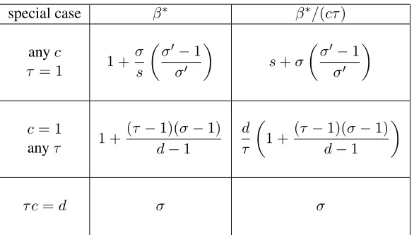
Here we comment in detail on the influence of the various design parameters (c = # computers,
special case β∗ β∗/(cτ)
anyc
τ = 1 1 +
σ s
σ0−1
σ0
s+σ
σ0−1
σ0
c= 1
anyτ 1 +
(τ −1)(σ−1)
d−1
d τ
1 +(τ−1)(σ−1)
d−1
τ c=d σ σ
Table 2: Stepsize parameterβ =β∗ and the leading factor in the rate (14) (assumingµR = 0) for several special cases of Hydra.
5.2 Strong Convexity
Notice that the size ofµR >0mitigates the effect of a possibly largeβon the bound (14). Indeed, for largeµR, the factor(β+µR)/(µf +µR)approaches 1, and the bound (14) is dominated by the term cτd, which means that Hydra enjoys linear speedup incandτ. In the following comments we will assume thatµR= 0, and focus on studying the dependence of the leading termdcτβ on various quantities, includingτ, c, σandσ0.
5.3 Search for Small but Safeβ
As shown by Tak´aˇc et al. (2013, Section 4.1), mini-batch SDCA mightdivergein the setting with
µf = 0 andR(x) ≡ 0, even for a simple quadratic function withd = 2, provided that β = 1. Hence, small values ofβneed to be avoided. However, in view of Theorem 5, it is good ifβ is as small as possible. So, there is a need for a “safe” formula for a smallβ. Our formula (10),β=β∗, is serving that purpose. For a detailed introduction into the issues related to selecting a goodβ for parallel coordinate descent methods, we refer the reader to the first 5 pages of (Fercoq and Richt´arik, 2013).
5.4 The Effect ofσ0
Ifc = 1, then by Lemma 9, σ0 = c = 1, and henceβ∗2 = 0. However, forc > 1 wemay have
β2∗ >0, which can hence be seen as a price we need to pay for using more nodes. The price depends on the way the data is partitioned to the nodes, as captured byσ0. In favorable circumstances,σ0 ≈1 even ifc > 1, leading to β2∗ ≈ 0. However, in general we have the boundσ0 ≥ cσ
d, which gets worse ascincreases and, in fact,σ0can be as large asc. Note also thatξis decreasing inτ, and that
100 101 102 103 100
101 102 103 104
σ
β
d / (c
τ
)
τ=1600 τ=12800 τ=105
(a)(c, s) = (1,105)
100 101 102 103
100 101 102 103 104
σ
β
d / (c
τ
)
τ=16 τ=128 τ=1000
(b)(c, s) = (102,103)
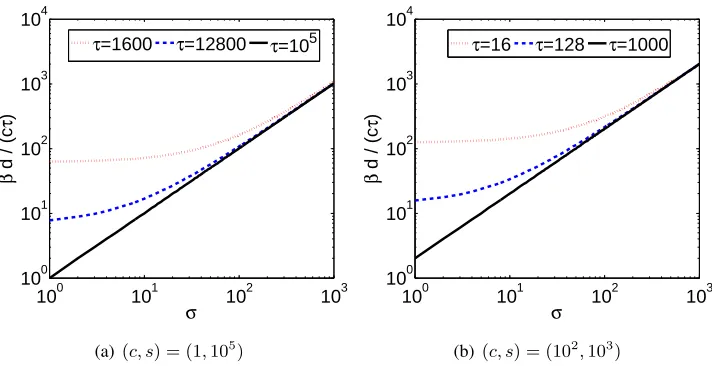
Figure 1: In terms of the number of iterations, very little is lost by usingc >1as opposed toc= 1.
with smallσ0. Due to the wayσ0is defined, this may not be an easy task. However, it may be easier to find partitions that minimizeω0, which is often a good proxy forσ0. Alternatively, we may ignore estimatingσ0altogether by settingβ = 2β∗1, as mentioned before, at the price of at most doubling the number of iterations.
5.5 Speedup by Increasingτ
Let us fixcand compare the quantitiesγτ := β ∗
cτ forτ = 1andτ =s. We now show thatγ1 ≥γs, which means that if all coordinates are updated at every node, as opposed to one only, then Hydra run withβ =β∗ will take fewer iterations. Comparing the 1st and 3rd row of Table 2, we see that
γ1 =s+σσ
0−1
σ0 andγs=σ. By Lemma 1,γ1−γs=s−σσ0 ≥0.
5.6 Price of Distribution
For illustration purposes, consider a problem withd= 105coordinates. In Figure 1(a) we depict the size of dβ∗1
cτ forc= 1and several choices ofτ, as a function ofσ. We see that Hydra works better for small values of σ and that with increasingσ, the benefit of using updating more coordinates diminishes. In Figure 1(a) we consider the same scenario, but withc= 100ands= 1000, and we plot d2β∗1
5.7 Comparison with Other Methods
While we are not aware of any otherdistributedcoordinate descent method, Hydra in thec= 1case is closely related to several existing parallel coordinate descent methods.
5.7.1 HYDRA VSSHOTGUN
The Shotgun algorithm (parallel coordinate descent) of Bradley et al. (2011) is similar to Hydra for
c = 1. Some of the differences: Bradley et al. (2011) only considerRequal to theL1norm and their method works in dimension2dinstead of the native dimensiond. Shotgun was not analyzed for strongly convexf, and convergence in expectation was established. Moreover, Bradley et al. (2011) analyze the step-size choiceβ = 1, fixed independently of the number of parallel updatesτ, and give results that hold only in a “smallτ” regime. In contrast, our analysis works for any choice ofτ.
5.7.2 HYDRA VSPCDM
Forc= 1, Hydra reduces to the parallel coordinate descent method (PCDM) of Richt´arik and Tak´aˇc (2015), but with abetterstepsize parameterβ. We were able to achieve smallerβ(and hence better rates) because we analyze a different and more specialized class of loss functions (those satisfy-ing (2)). In comparison, Richt´arik and Tak´aˇc (2015) look at a general class of partially separable losses. Indeed, in thec = 1 case, our distributed samplingSˆreduces to the sampling considered in (Richt´arik and Tak´aˇc, 2015) (τ-nice sampling). Moreover, our formula forβ (see Table 2) is essentially identical to the formula forβprovided in (Richt´arik and Tak´aˇc, 2015, Theorem 14), with the exception that we haveσwhere they haveω. By (9), we haveσ≤ω, and hence ourβis smaller.
5.7.3 HYDRA VSSPCDM
SPCDM of Fercoq and Richt´arik (2013) is PCDM applied to a smooth approximation of a nons-mooth convex loss; with a special choice ofβ, similar toβ1. As such, it extends the reach of PCDM
to a large class of nonsmooth losses, obtainingO(12) rates. It is possible to develop accelerated
Hydra withO(1)rates by combining ideas from this paper, Fercoq and Richt´arik (2013) with the APPROX method of Fercoq and Richt´arik (2015).
5.7.4 HYDRA VSMINI-BATCHSDCA
Tak´aˇc et al. (2013) studied the performance of a mini-batch stochastic dual coordinate ascent for SVM dual (“mini-batch SDCA”). This is a special case of our setup withc= 1, convex quadraticf
andRi(t) = 0fort∈[0,1]andRi(t) = +∞otherwise. Our results can thus be seen as a gener-alization of the results in that paper to a larger class of loss functionsf, more general regularizers
R, and most importantly, to the distributed setting (c >1). Also, we giveO(log1) bounds under strong convexity, whereas (Tak´aˇc et al., 2013) giveO(1)results without assuming strong convexity. However, Tak´aˇc et al. (2013) perform a primal-dual analysis, whereas we do not.
6. Distributed Computation of the Gradient
loss function` fi0(x) Mii
SL
m X
j=1
−Aji(yj−Aj:x) kA:ik22
LL
m X
j=1
−yjAji
exp(−yjAj:x)
1 + exp(−yjA j:x)
1 4kA:ik
2 2
HL X
j:yjAj
:x<1
−yjAji(1−yjAj:x)
kA:ik22
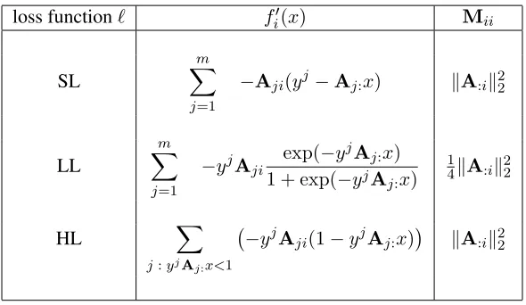
Table 3: Information needed in Step 5 of Hydra forf given by (3) in the case of the three losses`
from Table 1.
Note that in Hydra,xkis stored in a distributed way. That is, the valuesxikfori∈ Plare stored on computerl. Moreover, Hydra partitionsAcolumnwise asA= [A1, . . . ,Ac], whereAlconsists of columnsi∈ Pl ofA, and storesAl on computerl. So,Ais chopped into smaller pieces with stored in a distributed way in fast memory (if possible) across thecnodes. Note that this allows the method to work with large matrices.
At Step 5 of Hydra, node l at iteration k+ 1 needs to know the partial derivativesfi0(xk+1)
for i ∈ Sˆl ⊆ Pl. We now describe several efficient distributed protocols for the computation of fi0(xk+1) for functionsf of the form (3), in the case of the three losses` given in Table 1 (SL,
LL, HL). The formulas forfi0(x)are summarized in Table 3 (Aj:refers to thej-th row ofA). Let Dy := Diag(y).
6.1 Basic Protocol
If we writehi
k = 0ifiis not updated in iterationk, then
xk+1 =xk+ c X
l=1
X
i∈Slˆ
hikei. (16)
Now, if we let
gk:= (
Axk−y, for SL,
−DyAxk, for LL and HL,
(17)
then by combining (16) and (17), we get
gk+1=gk+ c X
l=1
δgk,l, where
δgk,l = (P
i∈Slˆ hikA:i, for SL, P
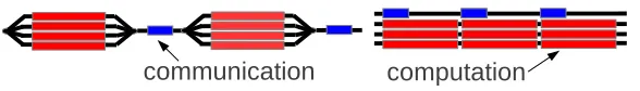
Figure 2: Parallel-serial (PS; left) vs Fully Parallel (FP; right) approach.
Note that the valueδgk,lcan be computed on nodelas all the required data is stored locally. Hence, we let each node computeδgk,l, and then use areduce alloperation to add up the updates to obtain gk+1, and pass the sum to all nodes. Knowinggk+1, nodelis then able to computefi0(xk+1)for
anyi∈ Plas follows:
fi0(xk+1) =
AT:igk+1=Pjn=1 Ajigjk+1, for SL,
Pn
j=1 yjAji
exp(gjk+1)
1+exp(gjk+1), for LL,
P
j:gjk+1>−1 y
jA
ji(1 +gkj+1), for HL.
6.2 Advanced Protocols
The basic protocol discussed above has obvious drawbacks. Here we identify them and propose modifications leading to better performance.
• alternating Parallel and Serial regions (PS):The basic protocol alternates between two pro-cedures: i) a computationally heavy one (done in parallel) with no MPI communication, and ii) MPI communication (serial). An easy fix would be to dedicate 1 thread to deal with com-munication and the remaining threads within the same computer for computation. We call this protocol Fully Parallel (FP). Figure 2 compares the basic (left) and FP (right) approaches.
• Reduce All (RA):In general, reduce all operations may significantly degrade the performance of distributed algorithms. Communication taking place only between nodes close to each other in the network, e.g., nodes directly connected by a cable, is more efficient. Here we propose theAsynchronous StreamLined (ASL)communication protocol in which each node, in a given iteration, sends only 1 message (asynchronously) to a nearby computer, and also receives only one message (asynchronously) from another nearby computer. Communication hence takes place in anAsynchronous Ring. This communication protocol requires significant changes in the algorithm. Figure 3 illustrates the flow of messages at the end of the k-th iteration forc= 4.
We order the nodes into a ring, denotingl−andl+the two nodes neighboring nodel. Nodel
only receives data froml−, and sends data tol+. Let us denote byδGk,lthe data sent by node ltol+at the end of iterationk. Whenlstarts iterationk, it already knowsδGk−1,l−.2 Hence, data which will be sent at the end of thek-th iteration by nodelis given by
δGk,l =δGk−1,l−−δgk−c,l+δgk,l. (18)
This leads to the update rule
gk+1,l =gk,l+δgk,l+δGk,l−−δgk−c+1,l.
Figure 3: ASL protocol withc= 4nodes. In iterationk, nodelcomputesδgk,l, and sendsδGk,lto l+.
ASL needs less communication per iteration. On the other hand, information is propagated more slowly to the nodes through the ring, which may adversely affect the number of itera-tions till convergence (note that we do not analyze Hydra with this communication protocol). Indeed, it takesc−1iterations to propagate information to all nodes. Also, storage require-ments have increased: at iterationkwe need to store the vectorsδgt,l fork−c ≤t ≤kon computerl.
7. Experiments
In this section we present numerical evidence that Hydra is capable to efficiently solve big data problems. We have a C++ implementation, using Boost::MPI and OpenMP. Experiments were executed on a Cray XE6 cluster with 128 nodes; with each node equipped with two AMD Opteron Interlagos 16-core processors and 32 GB of RAM.
7.1 Performance of Communication Protocols
In this experiment we consider a LASSO problem, i.e.,f given by (3) with`being the square loss (SL) and R(x) = kxk1. In order to to test Hydra under controlled conditions, we adapted the LASSO generator proposed by Nesterov (2013, Section 6); modifications were necessary as the generator does not work well in the big data setting.
As discussed in Section 6, the advantage of the RA protocol is the fact that Theorem 5 was proved in this setting, and hence can be used as a safe benchmark for comparison with the advanced protocols.
Table 4 compares the average time per iteration for the 3 approaches and 3 choices ofτ. We used128nodes, each running 4 MPI processes (hencec= 512). Each MPI process runs 8 OpenMP threads, giving 4,096 cores in total. The data matrixAhasn= 109rows andd= 5×10⁸columns, and has 3 TB, double precision. One can observe that in all cases, ASL-FP yields largest gains compared to the benchmark RA-PS protocol. Note that ASL has some overhead in each iteration, and hence in cases when computation per node is small (τ = 10), the speedup is only 1.62. When
τ comm. protocol organization avg. time speedup
10 RA PS 0.040 —
10 RA FP 0.035 1.15
10 ASL FP 0.025 1.62
102 RA PS 0.100 —
102 RA FP 0.077 1.30
102 ASL FP 0.032 3.11
103 RA PS 0.321 —
103 RA FP 0.263 1.22
103 ASL FP 0.249 1.29
Table 4: Duration of a single Hydra iteration for 3 communication protocols. The basic RA-PS protocol is always the slowest, but follows the theoretical analysis. ASL-FP can be 3×
faster.
is 3.11 times faster than RA-PS. But the gain becomes again only moderate forτ = 103; this is because computation now takes much longer than communication, and hence the choice of strategy for updating the auxiliary vectorgkis less significant. Let us remark that the use of largerτrequires larger beta, and hence possibly more iterations (in the worst case).
We now move on to solving an artificial big data LASSO problem with matrix A in block angular form, depicted in (19).
A=
Aloc1 0 · · · 0
0 Aloc2 · · · 0 ..
. ... . .. ... Aglob1 Aglob2 · · · Aglobc
. (19)
Such matrices often arise in stochastic optimization. Each Hydra head (=node) l owns two matrices: Alocl ∈R1,952,148×976,562andAglobl ∈R500,224×976,562. The average number of nonzero elements per row in the local part ofAlis175, and1,000for the global part. Optimal solutionx∗
has exactly160,000nonzero elements. Figure 4 compares the evolution ofL(xk)−L∗for ASL-FP and RA-FP.
Remark: When communicatinggkl, only entries corresponding to the global part ofAlneed to be communicated, and hence in RA, areduce alloperation is applied to vectorsδgglob,l ∈R500,224. In ASL, vectors with the same length are sent.
7.2 Updating All Coordinates on Each Node in Each Iteration Might not be Optimal
In this section we give an experimental demonstration that it may not be optimal for each node of Hydra to update all coordinates it owns (in each iteration). That is, we will show that the seemingly ideal choiceτ =sis not necessarily optimal.
fea-0 500 1000 1500 2000 10−10
100 1010
Elapsed Time [s]
L(x
k
)−L
* ASL−FP
RA−FP
Figure 4: Evolution ofL(xk)−L∗ in time. ASL-FP significantly outperforms RA-FP. The lossL is pushed down by 25 degrees of magnitude in less than 30 minutes (3TB problem).
0 20 40 60 80 100
10−8 10−6 10−4 10−2 100
Epochs
Duality gap
τ=2
τ=4
τ=8
τ=128
τ=256
0 200 400 600 800 1000
10−3
10−2
10−1
100
Iterations
Duality gap
τ=2
τ=4
τ=8
τ=128
τ=256
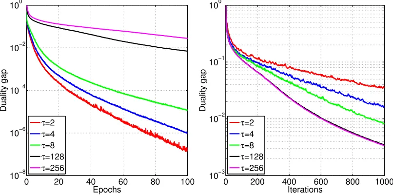
Figure 5: Evolution of the duality gap for several choices ofτ.
tures; and hence is a relatively small data set. We have chosen a random partition of the coordinates (=samples) toc = 32nodes, with each partition consisting ofs = 933samples (the last partition consists of959samples).
In Figure 5 we depict the evolution of the duality gap as a function of effective passes over data (epochs) (left plot) and as a function of iterations (right right). In each plot, we depict the performance of Hydra run with various choices ofτ.
1010 101 102 103 1.5
2 2.5 3
τ
(τβ*(1))/β*(τ)
Figure 6: Evolution of the duality gap for several choices ofτ.
of this situation is depicted in the right plot. That is, asτ increases, one needs fewer iterations to obtain any given accuracy.
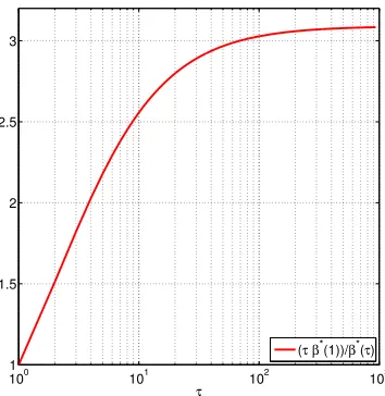
In Figure 6 we depict the theoretical speed-up guarantee, i.e., the fraction βτ∗. Looking at the right plot of Figure 5, we see that the choice τ = 256 does not lead to further speedup when compared to theτ = 128 choice. This phenomenon is also captured in Figure 6, where the line becomes quite flat aboveτ ≈102.
.
Remark: We have used10iterations of the power method in order to estimate parametersσand
σ0which were used to obtainβ∗using (10) (note that, in view of Lemma 2, we could have also used
β = 2β1∗). Their values are: σ= 440.61andσ0= 29.65.
7.3 A Simple Model for Communication-Computation Trade-Off: Search for Optimalτ
Assume allc nodes of the cluster are identical. Also assume s ≥ 2. Further, assume there is a constant1≤K ≤ssuch that while each node is able to computeKcoordinate updates in timeT1,
the computation ofjKupdates, forj= 2,3, . . . takesjT1units of time. This will be approximately
true in reality forKsufficiently large, typically a small multiple of the number of cores. It may be useful to think thatK is, in fact, equal to the number of cores of each node. Further, assume that the time of updatinggktogk+1 isT2(note that this involves communication).
Bases on this simple model, a single iteration of Hydra run withτ =jKcoordinate updates on each node (for1≤j≤s/K) takes
jT1+T2 (20)
units of time.
In what follows, we will assume, for simplicity, thatµR= 0(i.e., the regularizer is not strongly convex). The computations simplify with this assumption, but similar computations can be per-formed in theµR>0case.
100 101 102 100
101
j
z(j)
r1,2=10−4
r1,2=10−3
r1,2=10−2
r1,2=10−1
r1,2=100
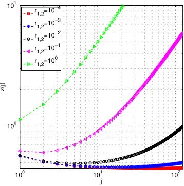
Figure 7: The dependence of the total “time complexity” T(j) on j for various values of the computation-communication ratior1,2.
time, as a function ofj, is proportional to
T(j) := β
jK(jT1+T2)
(10)
=
1 +(jK−1)(s σ−1)
1 +
jK
s − jK−1
s1
σ0−1
σ0 σ
jK (T2+T1j)
=
1 +(jK−1)(s σ−1)
1 +
jK
s − jK−1
s1
σ0−1
σ0 σ
jK (1 +jr1,2),
where
r1,2:= T1 T2 .
Note thatr1,2 is high if computation is expensive relative to communication, and vice versa. This
ratio can be estimated in any particular distributed system.
In Figure 7 we plotT(j)as a function ofjforr1,2 ∈ {10−4,10−3,10−2,10−1,100},K = 8and
the rest of the parameters appearing in the definition ofT(j)identical to those used in Section 7.2. For large enough r1,2, i.e., if communication is relatively cheap, thenT is an increasing function
ofj. This means that it is optimal to choosej = 1, which means that it is optimal to only update
τ =jKcoordinates on each node in each iteration. This observation is informally summarized as follows:
If communication is inexpensive relative to computation, it is optimal for each node to perform a small number of coordinate updates in each iteration. That is, if communi-cation is cheap, do less computation in each iteration.
10−4 10−3 10−2 10−1 100 0
50 100 150 200 250 300 350 400
r1,2
j
*(r
1,2
)
σ=10
σ=100
σ=1000
10−4 10−3 10−2 10−1 100
10−1 100 101 102 103
r1,2
j
*(r
1,2
)
σ=10
σ=100
σ=1000
Figure 8: Comparison ofj∗(r1,2)for various values of parameterσ(left: semilog plot; right: loglog
plot).
As communication becomes more expensive relative to computation, it is optimal for each node to perform a larger number of coordinate updates in each iteration. That is, if communication is more expensive, do more computation in each iteration.
SinceT is a simple function ofj, it is possible to findj∗which minimizesT(j)in closed form (if we relax the requirement of keepingjintegral, which is not very important):
j∗:= arg min
j T(j) = s
s(sσ0−σ)
r1,2K(sσ0(σ−1) +σ−σ0σ) .
In Figure 8 we plotj∗as a function ofr1,2forσ = 10,100,1000. Recall that smallerσmeans
less correlated data. This means that less synchronization is needed, and eventually allows us to do more coordinate updates in a single iteration (i.e.,j∗ is larger). If communication is relatively expensive (r1,2 is small), thenj∗is big. However, as communication gets cheaper,j∗ gets smaller.
7.4 Experiments with a Real Data Set in a Real Distributed Environment
In this section we report on experiments with the WebSpam data set Libsvm. This data set encodes a binary classification problem with d = 350,000samples and n = 16,609,143 features. The total size of the data set describing the problem exceeds 23 GB. We split this data into c = 16 balanced groups, each containing s = 21,875 samples and applied Hydra to the problem (the dual of SVM with hinge loss) for various choices ofτ. The results are depicted in Figure 9. As each node in our experiments had an 8-core processor, we have chosenτ in multiples of 8: τ ∈ {8,80,160,320,640,1280,2560,5120}.
In the plot on the left we have run the RA variant withβ := 2β1∗ and in the plot on the right we have run the RA withβ := 2β
∗
1
100. By comparing the plots, we can observe that for this particular
0 500 1000 10−3
10−2 10−1 100
Elapsed time [sec.]
Duality gap
τ=8
τ=80
τ=160
τ=320
τ=640
τ=1280
τ=2560
τ=5120
0 500 1000
10−6 10−4 10−2 100
Elapsed time [sec.]
Duality gap
τ=8
τ=80
τ=160
τ=320
τ=640
τ=1280
τ=2560
τ=5120
Figure 9: The duality gap evolving in time for Hydra run with various levels of parallelism (as given byτ) within each node.
can be obtained by using a more aggressive stepsize strategy, i.e., by choosingβ hundred times smaller than the one recommended by theory. While it is to be expected that particular data sets will tolerate such aggressive stepsize strategies, there are data sets where such stepsizes might lead to a diverging algorithm. However, it is clear that Hydra would benefit from a line-search procedure for the selection ofβ.
One can also observe from Figure 9 that with beyond some point, increasingτ does not bring much benefit, and only increases the runtime.
8. Extensions
Our results can be extended to the setting where coordinates are replaced by blocks of coordinates, as in (Nesterov, 2012), and to partially separable losses, as in (Richt´arik and Tak´aˇc, 2015). We expect the block setup to potentially lead to further significant speedups in a practical implementa-tion due to the fact that this will allow us to design data-dependent block norms, which will in turn enable Hydra to use more curvature information the information contained in the diagonal ofM. In such a setup, in Step 7 we will instead have a problem of a larger dimension, and the quadratic term can involve a submatrix ofM.
Acknowledgements
Appendix A. Proof Lemma 1
1. The inequality ω0 ≤ c is obviously true. By considering x with zeroes in all coordinates except those that belong toPk(wherekis an arbitrary but fixed index), we see thatxTQx=
xTBQx, and henceσ0≥1.
2. We now establish thatσ0 ≤ω0. Letφ(x) = 12xTQx,x∈Rd; its gradient is
φ0(x) =Qx. (21)
For eachk= 1,2, . . . , c, define a pair of conjugate norms onRsas follows:
kvk2
(k):=hQkkv, vi, (kvk ∗
(k))2:=k max
v0k
(k)≤1
hv0, vi=h(Qkk)−1v, vi. (22)
LetUkbe a column submatrix of thed-by-didentity matrix corresponding to columnsi∈ Pk. Clearly,Ak =AUkandUTkQUkis thek-th diagonal block ofQ, i.e.,
UTkQUk
(4)
=Qkk. (23)
Moreover, for x ∈ Rd andk ∈ {1,2, . . . , c}, letx(k) = UT
kx and, fixing positive scalars w1, . . . , wc, define a norm onRdas follows:
kxkw := c X
k=1
wkkx(k)k2(k)
!1/2
. (24)
Now, we claim that for eachk,
kUTkφ0(x+Ukh(k))−UTkφ0(x)k∗(k) ≤ kh (k)k
(i).
This means that φ0 is block Lipschitz (with blocks corresponding to variables inPk), with respect to the normk · k(k), with Lipschitz constant1. Indeed, this is, in fact, satisfied with equality:
kUTkφ0(x+Ukh(k))−UTkφ0(x)k∗(k) (21)
= kUTkQ(x+Ukh(k))−UkQxk∗(k)
= kUTkQUkh(k)k∗(k)
(23)
= kQkkh(k)k∗(k)
(22)
= h(Qkk)−1Qkkh(k),Qkkh(k)i (22)
= kh(k)k(k).
This is relevant because then, by Richt´arik and Tak´aˇc (2015, Theorem 7; see comment 2 following the theorem), it follows thatφ0 is Lipschitz with respect tok · kw, wherewk = 1 for allk= 1, . . . , c, with Lipschitz constantω0(ω0is the degree of partial block separability ofφwith respect to the blocksPk). Hence,
1 2x
TQx=φ(x)≤φ(0)+(φ0
(0))Tx+ω
0
2 kxk
2
w
(22)+(24)
= ω
0
2 c X
k=1
hQkkx(k), x(k)i= ω
0
2(x
TBQx),
3. We now show that σs ≤σ0. If we letθ:= max{xTBQx:xTx ≤1}, thenxTBQx≤θxTx
and hence{x : xTx≤1} ⊆ {x : xTBQx≤θ}. This implies that
σ= max x {x
TQx : xTx≤1} ≤max x {x
TQx : xTBQx≤θ}=θσ0.
It now only remains to argue thatθ ≤ s. Forx ∈ Rd, letx(k) denote its subvector in
Rs corresponding to coordinatesi ∈ Pkand∆ = {p ∈ Rc : p ≥ 0, Pc
k=1pk = 1}. We can now write
θ = max
x ( c
X
k=1
(x(k))TQkkx(k) : c X
k=1
(x(k))Tx(k)≤1 )
= max
p∈∆
c X
k=1
n
max(x(k))TQkkx(k) : (x(k))Tx(k) =pk o
= max
p∈∆
c X
k=1
pkmax n
(x(k))TQkkx(k) : (x(k))Tx(k)= 1o
= max
1≤k≤cmax n
(x(k))TQkkx(k) : (x(k))Tx(k)= 1o
≤ s.
In the last step we have used the fact thatσ(Q) =σ≤c= dim(Q), proved in steps 1 and 2, applied to the settingQ←Qkk.
4. The chain of inequalities1≤σ ≤ω ≤cis obtained as a special case of the chain1 ≤σ0 ≤
References
J. Bradley, A. Kyrola, D. Bickson, and C. Guestrin. Parallel coordinate descent for l1-regularized loss minimization. InICML, 2011.
O. Fercoq. Parallel coordinate descent for the AdaBoost problem. InICMLA, 2013.
O. Fercoq and P. Richt´arik. Smooth minimization of nonsmooth functions with parallel coordinate descent methods. arXiv:1309.5885, 2013.
O. Fercoq and P. Richt´arik. Accelerated, parallel and proximal coordinate descent. SIAM Journal on Optimization, 25(4):1997–2023, 2015.
C-J. Hsieh, K-W. Chang, C-J. Lin, S.S. Keerthi, , and S. Sundarajan. A dual coordinate descent method for large-scale linear SVM. InICML, 2008.
Libsvm. Datasets. http://www.csie.ntu.edu.tw/∼cjlin/ libsvmtools/datasets/binary.html.
Z. Lu and L. Xiao. On the complexity analysis of randomized block-coordinate descent methods. Mathematical Programming, 152(1):615–642, 2015.
I. Mukherjee, Y. Singer, R. Frongillo, and K. Canini. Parallel boosting with momentum. InECML, 2013.
I. Necoara, Yu. Nesterov, and F. Glineur. Efficiency of randomized coordinate descent methods on optimization problems with linearly coupled constraints. Technical report, 2012.
Yu. Nesterov. Efficiency of coordinate descent methods on huge-scale optimization problems.SIAM Journal on Optimization, 22(2):341–362, 2012.
Yu. Nesterov. Gradient methods for minimizing composite objective function. Mathematical Pro-gramming, 140(1):125–161, 2013.
P. Richt´arik and M. Tak´aˇc. Parallel coordinate descent methods for big data optimization. Mathe-matical Programming, pages 1–52, 2015.
P. Richt´arik and M. Tak´aˇc. Efficient serial and parallel coordinate descent methods for huge-scale truss topology design. InOperations Research Proceedings, pages 27–32. Springer, 2012.
P. Richt´arik and M. Tak´aˇc. Iteration complexity of randomized block-coordinate descent methods for minimizing a composite function. Mathematical Programming, 144(2):1–38, 2014.
S. Shalev-Shwartz and A. Tewari. Stochastic methods for `1 regularized loss minimization. In
ICML, 2009.
S. Shalev-Shwartz and T. Zhang. Accelerated mini-batch stochastic dual coordinate ascent. InNIPS, pages 378–385, 2013a.
S. Shalev-Shwartz, Y. Singer, N. Srebro, and A. Cotter. Pegasos: Primal estimated sub-gradient solver for SVM. Mathematical Programming, 127(1):3–30, 2011.
M. Tak´aˇc, A. Bijral, P. Richt´arik, and N. Srebro. Mini-batch primal and dual methods for SVMs. In ICML, 2013.
R. Tappenden, P. Richt´arik, and J. Gondzio. Inexact coordinate descent: complexity and precondi-tioning. arXiv:1304.5530, 2013.