Estimation of Graphical Models through Structured Norm
Minimization
Davoud Ataee Tarzanagh [email protected]
Department of Mathematics UF Informatics Institute University of Florida
Gainesville, FL 32611-8105, USA
George Michailidis [email protected]
Department of Statistics UF Informatics Institute University of Florida
Gainesville, FL 32611-8545, USA
Editor:Bert Huang
Abstract
Estimation of Markov Random Field and covariance models from high-dimensional data represents a canonical problem that has received a lot of attention in the literature. A key assumption, widely employed, is that of sparsityof the underlying model. In this paper, we study the problem of estimating such models exhibiting a more intricate structure com-prising simultaneously ofsparse, structured sparseanddensecomponents. Such structures naturally arise in several scientific fields, including molecular biology, finance and political science. We introduce a general framework based on a novel structured norm that enables us to estimate such complex structures from high-dimensional data. The resulting opti-mization problem is convex and we introduce a linearized multi-block alternating direction method of multipliers (ADMM) algorithm to solve it efficiently. We illustrate the superior performance of the proposed framework on a number of synthetic data sets generated from both random and structured networks. Further, we apply the method to a number of real data sets and discuss the results.
Keywords: Markov Random Fields, Gaussian covariance graph model, structured sparse norm, regularization, alternating direction method of multipliers (ADMM), convergence.
1. Introduction
There is a substantial body of literature on methods for estimating network structures from high-dimensional data, motivated by important biomedical and social science applications; see Barab´asi and Albert (1999); Liljeros et al. (2001); Robins et al. (2007); Guo et al. (2011a); Danaher et al. (2014); Friedman et al. (2008); Tan et al. (2014); Guo et al. (2015). Two powerful formalisms have been employed for this task, the Markov Random Field (MRF) model and the Gaussian covariance graph model (GCGM). The former captures statistical conditional dependence relationships amongst random variables that correspond to the net-work nodes, while the latter to marginal associations. Since in most applications the number of model parameters to be estimated far exceeds the available sample size, the assumption
c
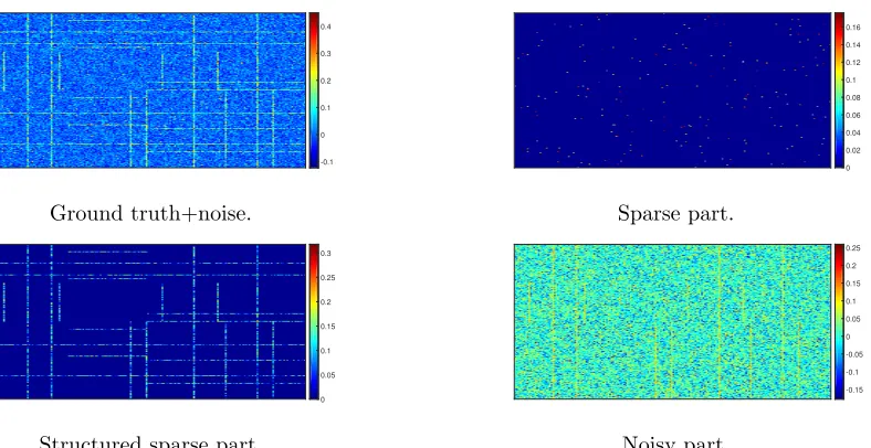
of sparsity is made and imposed through regularization. An `1 penalty on the parame-ters encoding the network edges is the most common choice; see Friedman et al. (2008); Karoui (2008); Cai and Liu (2011); Xue et al. (2012), which can also be interpreted from the Bayesian perspective as using an independent double-exponential prior distribution on each edge parameter. Consequently, this approach encourages sparse uniform network structures that may not be the most suitable choice for many real world applications, which in turn havehubnodes ordense subgraphs. As argued in Barab´asi and Albert (1999); Liljeros et al. (2001); Newman (2001); Li et al. (2005); Fortunato (2010); Newman (2012) many networks exhibit different structures at different scales. An example includes a densely connected subgraph, also known as acommunity in the social networks literature. Such structures in social interaction networks may correspond to groups of people sharing common interests or being co-located (Traud et al., 2011; Newman and Girvan, 2004), while in biological systems to groups of proteins responsible for regulating or synthesizing chemical products (Guimera and Amaral, 2005; Lewis et al., 2010; see, Figure 3 for an example). Hence, in many applications, simple sparsity or alternatively, a dense structure fails to capture salient features of the true underlying mechanism that gave rise to the available data.
In this paper, we introduce a framework based on a novel structured sparse norm that allows us to recover such complex structures. Specifically, we consider Markov Random Field and covariance models where the parameter of interest, Θ can be expressed as the superposition of sparse, structured sparse and dense components as follows:
Θ = Z1+Z1> | {z } sparse part
+ Z2+Z2>+· · ·+Zn+Zn>
| {z }
structured sparse part
+ E
|{z} dense part
, (1)
where Z1 is a sparse matrix, Z2, . . . , Zn are the set of n−1 structured sparse matrices (see, Figure 3 for an example of such structured matrices), andE is a dense matrix having possibly very many small, non-zero entries. As shown in Figure 3, the elements of Z1 represent edges between non-structured nodes, and the non-zero parts of structured matrices Z2, . . . , Zn correspond to densely connected subgraphs (communities).
We elaborate more on the decomposition proposed above. We start by discussing on the sparse and structured sparse component and then elaborate on the dense component. Traditional sparse (lasso Tibshirani, 1996; Friedman et al., 2008) and group sparse (group lasso Yuan and Lin, 2007; Jacob et al., 2009; Obozinski et al., 2011) are tailor-made to estimate and recover sparse and structured sparse model structures, respectively. However, these methods can not accommodate different structures, unless users specify a priorithe structure of interest (e.g. hub nodes and sparse components), thus severely limiting their application scope. On the other hand, the general framework introduced, is capable of estimating from high-dimensional data, groups with overlaps, hubs and dense subgraphs, with the size and location of such structures not known a priori.
tuning to recover the sparse component of interest. This line of reasoning is also adopted in Chernozhukov et al. (2017). Note however, that the model may also be used in settings where there is a significant dense component; however, as discussed in Chernozhukov et al. (2017) recovery of the individual component is not guaranteed. Hence, in this work we adopt the viewpoint that E represents a small ”perturbation” of the sparse+structured sparse structure. To achieve these goals, it leverages a new structured norm that is used as the regularization term of the corresponding objective function.
The resulting optimization problem is solved through a multi-block ADMM algorithm. A key technical innovation is the development of a linearized ADMM algorithm that avoids introducing auxiliary variables which is a common strategy in the literature. We estab-lish the global convergence of the proposed algorithm and illustrate its efficiency through numerical experimentation. The algorithm takes advantage of the special structure of the problem formulation and thus is suitable for large instances of the problem. To the best of our knowledge, this is the first work that gives global convergence guarantees for linearized multi-block ADMM with Gauss-Seidel updates, which is of interest in its own accord.
The remainder of the paper is organized as follows: In Section 2, we present the new structured norm used as the regularization term in the objective function of the Markov Random Field, covariance graph, regression and vector auto-regression models. In Section 3, we introduce an efficient multi-block ADMM algorithm to solve the problem, and provide the convergence analysis of the algorithm. In Section 4, we illustrate the proposed framework on a number of synthetic and real data sets, while some concluding remarks are drawn in Section 5.
2. A General Framework for Learning under Structured Sparsity
We start by introducing key definitions and associated notation.
2.1 Symmetric Structured Overlap Norm
LetX be an m×pdata matrix, Θ be ap×psymmetric matrix containing the parameters of interest of the statistical loss function G(X,Θ). The most popular assumption used in the literature is that Θ is sparseand can be successfully recovered from high-dimensional data by solving the following optimization problem
minimize
Θ∈S G(X,Θ) +λ
Θ
1, (2)
where S is some set depending on the loss function; λ is s a non-negative regularization constant; and k.k1 denotes the `1 norm or the sum of the absolute values of the matrix elements.
To explicitly model different structures in the parameter Θ, we introduce the following
symmetric structured overlap norm (SSON):
for a set of partitioned matrices Z1, . . . , Zn is given by, minimize
Z1,...,Zn, E
Ω(Θ, Z1, . . . , Zn, E) := λ1kZ1−diag(Z1)k1
+ n X
i=2 ˆ
λikZi−diag(Zi)k1+λi li
X
j=1
k(Zi−diag(Zi))jkF
+ λe 2 kEk
2 F, Θ = n X i=1
Zi+Zi>
+E, (3)
where {λi}ni=1 and {λˆi}ni=2 are nonnegative regularization constants; li is the number of
blocks of the partitioned matrixZi;(Zi−diag(Zi))j is thejth block of the partitioned matrix Zi; E is an unstructured noise matrix;k.k1 denotes the `1 norm or the sum of the absolute
values of the matrix elements; and k.kF the Frobenius norm.
We note that the overlap norm defined by Mohan et al. (2012); Tan et al. (2014) en-courages the recovery of matrices that can be expressed as a union of few rows and the corresponding columns (i.e. hub nodes). However, SSON represents a new symmetric and significantly more general variant of the overlap norm that promotes matrices that can be expressed as the sum of symmetric structured matrices. Moreover, unlike the previous group sparsity and the latent group lasso discussed in Yuan and Lin (2007); Jacob et al. (2009); Obozinski et al. (2011) that require users to specify structures of interesta priori, the SSON achieves a similar objective in anagnostic manner, relying only on how well such structures fit the observed data.
In many applications, such as regression models, we are interested in modeling different structures in a parameter vector θ. In these cases, we have the following definition as a special case of SSON:
Definition 2 Let θ be a p×1 vector containing the model parameters of interest. The structured overlap norm for a set of partitioned vectors z1, . . . , zn is given by,
minimize z1,...,zn, e
ω(θ, z1, . . . , zn, e) := λ1kz1k1+ n X
i=2 ˆ
λikzik1+λi li
X
j=1
kzijk2+ λe
2 kek 2 2,
θ = z1+z2+· · ·+zn+e, (4)
where {λi}ni=1 and {λˆi}ni=2 are nonnegative regularization constants; li is the number of
blocks of the partitioned vector zi; zij is the jth block of the partitioned vector zi (see, Figure 1); e is an unstructured noise vector; k.k1 denotes the `1 norm or the sum of the
absolute values of the vector elements; andk.k2 the two norm.
Remark 3 In the formulation of the problem, λ1, {λˆ2, . . . ,λˆn, λ2, . . . , λn}, and λe are
tuning parameters corresponding to the sparse component Z1, the structured components
{Z2, . . . Zn} and the dense (noisy) component E, respectively. While the nonzero
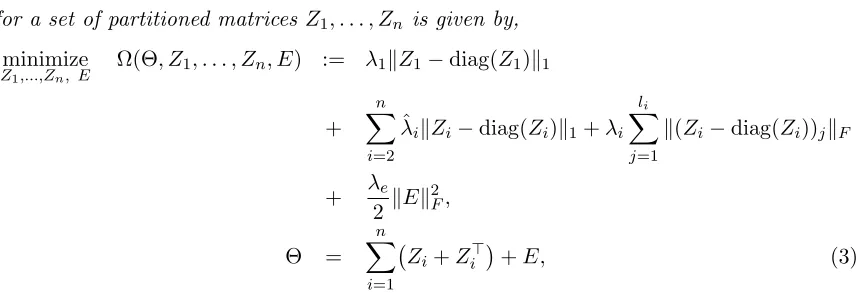
Figure 1: Decomposition of a vector θ into partitioned vectors z1, z2 and z3, where z1 is sparse, z2 and z3 are structured sparse vectors. White and red elements are zero and non-zero in the model parameter vector θ, respectively.
Remark 4 The SSON admits the lasso (Tibshirani, 1996), the group lasso with overlaps (Jacob et al., 2009; Obozinski et al., 2011) and the ridge shrinkage (Hoerl and Kennard, 1970) methods as three extreme cases, by respectively setting {λˆ2, . . . ,λˆn, λ2, . . . , λn, λe} →
∞, {λ1,λˆ2, . . . ,λˆn, λe} → ∞, and{λ1, . . . , λn,λˆ2, . . . ,λˆn} → ∞1.
Note that SSON is rather different from the sparse group lasso, which also uses a com-bination of `1 and `G penalization, where k.kG is the group lasso norm. The sparse group lasso penalty is ¯ω(θ) = λ1kθk1 +λ2kθkG, and thus the includes lasso and group lasso as extreme cases corresponding to λ2 = 0 and λ1 = 0, respectively. However, ¯ω(θ) does not split θ into a sparse and a group sparse part and will produce a sparse solution as long as λ1>0. Hence, the sparse group lasso method can be thought of as a sparsity-based method with additional shrinkage bykθkG. The group sparsity processes data very differently from SSON and consequently has very different prediction risk behavior. The same argument illustrates the advantages of the proposed SSON penalty over the well-known elastic net penalty. The elastic net is a combination of lasso and ridge penalties (Zou and Hastie, 2005). However, the elastic net does not split θinto a sparse and a dense component. Our results show that SSON tends to perform no worse than, and often performs significantly better than ridge, lasso, group lasso or elastic net with penalty levels chosen by cross-validation.
Remark 5 In order to encourage different structures in the parameter matrix Θ, we con-sider the Frobenius norm of blocks of partitioned matrices, which leads to recovery of dense subgraphs. Other values for the norm of such blocks are also possible; e.g. the`∞ norm.
Remark 6 The matrix E is an important component of the SSON framework.
It enables to develop a convergent multi-block ADMMto solve the problem of estimating a structured Markov Random Field or covariance model. Note that in general, a direct
extension of ADMM to multi-block convex minimization problems is not necessar-ily convergent even without linearization of the corresponding subproblems as shown in Chen et al. (2016).
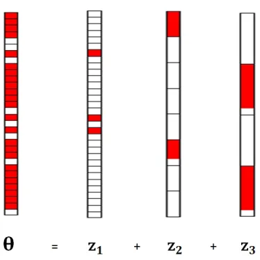
From a performance standpoint, our results show that adding a ridge penalty term λe
2 kEk 2 F
to the structured norm is provably effective in correctly identifying the underlying structures in the presence of noisy data (Zou and Hastie, 2005; Chernozhukov et al., 2017) (see, Figure 2 for an example of decomposition (1) in the presense of noise for covariance matrix estimation.)
-0.1 0 0.1 0.2 0.3 0.4
Ground truth+noise.
0 0.02 0.04 0.06 0.08 0.1 0.12 0.14 0.16
Sparse part.
0 0.05 0.1 0.15 0.2 0.25 0.3
Structured sparse part.
-0.15 -0.1 -0.05 0 0.05 0.1 0.15 0.2 0.25
Noisy part.
Figure 2: Heat map of the covariance matrix Θ3 decomposed into sparse and structured sparse parts in the presence of noise, estimated by SSON using problem (11).
Next, we discuss the use of the SSON as a regularizer for maximum likelihood estimation of the following popular statistical models: (i) members of the Markov Random Field family including the Gaussian graphical model, the Gaussian graphical model with latent variables and the binary Ising model, (ii) the Gaussian covariance graph model and (iii) the classical regression and the vector auto-regression models. For the sake of completeness, we provide a complete, but succinct description of the corresponding models and the proposed regularization.
2.2 Structured Gaussian Graphical Models
Let X be a data matrix consisting of p-dimensional samples from a zero mean Gaussian distribution,
x1, . . . , xm i.i.d.∼ N(0,Σ).
(a) Postpartum NAC Gene Network (Zhao et al., 2014).
Θ
Z1 ZT
1
Z2 Z2T
Z3 Z3T
(b)Examples of partitioned matrices for the underlying net-work in (a).
Figure 3: The figure illustrates that block partitions through structured matrices could be set based on a desire for interpretability of the resulting estimated network structure. Panel (a) shows example of structured gene network, while panel (b) provides decomposition into structured matrices for the network in (a). Blue elements are diagonal ones, white elements are zero and red elements are non-zero in the model parameter matrix Θ. The structured penalty function (3) is then applied to each block for matrices {Zi}ni=1.
graphical lasso problem (Friedman et al., 2008; Rothman et al., 2008) in the form of (2) with loss function
G1(X,Θ1) := trace( ˆΣΘ1)−log det Θ1, Θ1 ∈ S, (5) where ˆΣ is the empirical covariance matrix ofX; Θ1 is the estimate of the precision matrix Σ−1; and S is the set of p×p symmetric positive definite matrices.
As is well known, the norm penalty in (2) encourages zeros (sparsity) in the solution. However, as previously argued, many biological and social network applications exhibit more complex structures than mere sparsity. Using the proposed SSON, we define the following objective function for the problem at hand:
minimize Θ1,Z1,...,Zn∈S, E
G1(X,Θ1) + Ω(Θ1, Z1, . . . , Zn, E),
Θ1 = n X
i=1
Zi+Zi>
+E, (6)
where Θ1 is the model parameter matrix and Ω(Θ1, Z1, . . . , Zn, E) the corresponding SSON defined in (3).
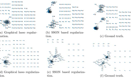
(a) Graphical lasso regular-ization.
(b) SSON based
regulariza-tion. (c) Ground truth.
(d) Graphical lasso regulariza-tion.
(e) SSON based
regulariza-tion. (f) Ground truth.
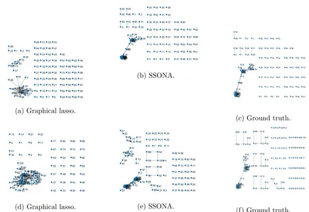
Figure 4: Estimates from the SSON based regularization on two examples of Gaussian graphical models comprising ofp= 100 nodes, using in (4b) three structured matrices and in (4e) four structured matrices.
In Figure 4, the performance of our proposed approach is illustrated on two simulated data sets exhibiting different structures (sub-figures (4c) and (4f)); it can be seen that the proposed SSON based graphical lasso (sub-figures (4b) and (4e)) can recover the network structure much better than the popular graphical lasso based estimator (Friedman et al., 2008) (subfigures (4a) and (4d)).
2.3 Structured Ising Model
Another popular graphical model, suitable for binary or categorical data, is the Ising one (Ising, 1925). It is assumed that observations x1, . . . , xm are independent and identically distributed from
f(x,Θ2) = 1
W(Θ2)
exp p X
j=1
θjjxj+ X
1≤j<j0≤p
θjj0xjxj0
, (7)
where W(Θ2) is the partition function, which ensures that the density sums to one. Here,
Θ2 is ap×p symmetric matrix that specifies the network structure: θjj0 = 0 implies that thejth and j0th variables are conditionally independent given the remaining ones.
proposed a neighborhood selection approach. The latter proposal involves solvingplogistic regressions separately (one for each node in the network), which leads to an estimated parameter matrix that is in general not symmetric. In contrast, several authors considered maximizing an `1-penalized pseudo-likelihood with a symmetric constraint on Θ2 (Guo et al., 2011a,b). Under the model (7), the log-pseudo-likelihood for m observations takes the form
G2(X,Θ2) := p X
j=1 p X
j0=1
θjj0(XTX)jj0− m X i=1 p X j=1
log1 + exp θjj+ X
j06=j
θjj0xij0
, (8)
We propose instead to impose the SSON on Θ2 in (8) in order to estimate a binary network with different structures. This leads to the following optimization problem
minimize Θ2,Z1,...,Zn∈S, E
G2(X,Θ2) + Ω(Θ2, Z1, . . . , Zn, E),
Θ2 = n X
i=1
Zi+Zi>
+E, (9)
where Θ2 is the model parameter matrix and Ω(Θ2, Z1, . . . , Zn, E) the corresponding SSON defined in (3).
An interesting connection can be drawn between our technique and the Ising block model discussed in Berthet et al. (2016), which is a perturbation of the mean field approximation of the Ising model known as the Curie-Weiss model: the sites are partitioned into two blocks of equal size and the interaction between those within the same block is stronger than across blocks, to account for more order within each block. However, one can easily seen that the Ising block model is a special case of (9).
2.4 Structured Gaussian Covariance Graphical Models
Next, we consider estimation of a covariance matrix under the assumption that
x1, . . . , xm i.i.d.
∼ N(0,Σ).
This is of interest because the sparsity pattern of Σ specifies the structure of the marginal independence graph (Drton and Richardson, 2002, 2008).
Let Θ3 be ap×p symmetric matrix containing the parameters of interest. Setting the loss functionG3(X,Θ3) :=
1 2kΘ3−
ˆ Σk2
F, Xue et al. (2012) proposed to estimate the positive definite covariance matrix, Σ by solving
minimize Θ3∈S
G3(X,Θ3) +λkΘ3k1, (10)
where ˆΣ is the empirical covariance matrix, S ={Θ3 : Θ3 εI and Θ3 = ΘT3}, and εis a small positive constant. We extend (10) to accommodate structures of the covariance graph by imposing the SSON on Θ3. This results in the following optimization problem
minimize Θ3,Z1,...,Zn∈S, E
G3(X,Θ3) + Ω(Θ3, Z1, . . . , Zn, E),
Θ3 = n X
i=1
Zi+Zi>
where Θ3 is the model parameter matrix and Ω(Θ3, Z1, . . . , Zn, E) the corresponding SSON defined in (3).
2.5 Structured Gaussian Graphical Models with latent variables
In many applications throughout science and engineering, it is often the case that some relevant variables are not observed. For the Gaussian Graphical model, Chandrasekaran et al. (2010) proposed a convex optimization problem to estimate it in the presence of latent variables. Let Θ4be ap×psymmetric matrix containing the parameters of interest. Setting
G4(X,Θ4) :=hΘ4,ΣOi −log det Θ4, their objective function is given by minimize
Θ4,Z1,Z2∈S
G4(X,Θ4) +αkZ1k1+βtrace(Zn+1) +1Zn+10,
Θ4 = Z1−Zn+1, (12)
where ΣO is the sample covariance matrix of the observed variables; α and β are positive constants; and the indicator function1Zn+10 is defined as
1Zn+10:=
(
0, ifZn+1 0, +∞, otherwise.
This convex optimization problem aims to estimate an inverse covariance matrix that can be decomposed into a sparse matrix Z1 minus a low-rank matrix Zn+1 based on high-dimensional data.
Next, we extend the SSON to solve the latent variable graphical model selection. Prob-lem (12) can be rewritten in the following equivalent form by introducing new variables
{Zi}ni=1: minimize Θ4,Z1,...,Zn∈S, E
G4(X,Θ4) + Ω(Θ4, Z1, . . . , Zn, E) +λn+1trace(Zn+1) +1Zn+10,
Θ4 = n X
i=1
Zi+Zi>
−Zn+1+E, (13)
where Θ4 is the model parameter matrix and Ω(Θ4, Z1, . . . , Zn, E) the corresponding SSON defined in (3).
2.6 Structured Linear Regression and Vector Auto-Regression
The proposed SSON is also applicable to structured regression problems. Although this is not the main focus on this paper, nevertheless, we include a brief discussion, especially for lag selection in vector autoregressive models that are of prime interest in the analysis of high-dimensional time series data. The canonical formulation of the regularized regression problem is given by:
min θ∈Rp
ky−Xθk2+λΨ(θ). (14)
choices of Ψ(.) lead to popular regularizers including the lasso -Ψ(θ) =kθk1- and the group lasso.
We propose instead to impose the SSON on θ in (14) in order to solve structured regression problems. Problem (14) can be rewritten in the following form by introducing new variables {zi}ni=1 and e:
minimize θ,z1,...,zn,e
G(X, θ) +ω(θ, z1, . . . , zn, e),
θ4 = z1+z2+· · ·+zn+e, (15)
where G(X, θ) = ky −Xθk2; θ is the model parameter vector and ω(θ, z1, . . . , zn, e) the corresponding structured norm defined in (4).
Problem (15) can equivalently be thought of as a generalization of subspace clustering (Elhamifar and Vidal, 2009). Indeed, in order to segment the data into their respective subspaces, we need to compute an affinity vector θ that encodes the pairwise affinities between data vectors.
An interesting application of the SSON for multivariate regression problems is on struc-tured estimation ofvector autoregression(VAR) models (L¨utkepohl, 2005), a popular model for economic and financial time series data (Tsay, 2005), dynamical systems (Ljung, 1998) and more recently brain function connectivity (Vald´es-Sosa et al., 2005). The model cap-tures both temporal and cross-dependencies between stationary time series. Formally, let
{x1, . . . , xm} be a p-dimensional time series set of observations that evolve over time ac-cording to a lag-dmodel:
xt+1 = d X
k=1
Θ>kxt−k+t, 1, . . . , m−1 i.i.d.
∼ N(0,Σ), t= 1, . . . , m−1,
where{Θ}d
k=1 ∈Rp
×paretransition matricesfor different lags, and{
1, . . . , m−1} indepen-dent multivariate Gaussianwhite noise processes. The VAR process is assumed to be stable and stationary (bounded spectral density), while the noise covariance matrix Σ is assumed to be positive definite with bounded largest eigenvalue (Basu and Michailidis, 2015).
Given m observations{x1, x2, . . . , xm} from a stationary VAR process, the lag-m VAR can be written is given by
xm xm−1
.. . x2
| {z } Y =
xm−1> xm−2>
.. . x1>
| {z } X Θ +
m−1> m−2>
.. . 1>
| {z } ε
. (16)
It can be seen that to estimate Θ one can solve the following least squares problem
min Θ∈Rp×p
kY −XΘkF. (17)
limited sample size. A popular choice is the lasso (Basu and Michailidis, 2015), that leads to sparse estimates. However, it does not incorporate the notion of lag selection, which could lead to certain spurious coefficients coming from further lags in the past. To address this problem, Basu et al. (2015) proposed a thresholded lasso estimate. However, our SSON can be used for lag selection, that guarantees that more recent lags are favored over further in the past ones.
Let Θ5 be a mp×mp symmetric matrix containing the parameters of interest for all m lages of the problem. Setting the loss functionG5(X,Θ5) :=kY −XΘ5k, we propose to estimate the transition matrix, Θ by solving the following optimization problem:
min Θ5,Z1,...,Zn,E∈Rp×p
G5(X,Θ5) + Ω(Θ5, Z1, . . . , Zn, E),
Θ5 = n X
i=1
Zi+Zi>
+E, (18)
where Θ5 is the estimate of the covariance matrix and Ω(Θ5, Z1, . . . , Zn, E) the correspond-ing SSON defined in (3).
3. Multi-Block ADMM for Estimating Structured Network Models
Objective functions (6), (9), (11), (13), (15), and (18) involve separable convex functions, while the constraint is simply linear, and therefore they are suitable for ADMM based algorithms. We next introduce a linearized multi-block ADMM algorithm to solve these problems and establish its global convergence properties.
The alternating direction method of multipliers (ADMM) is widely used in solving struc-tured convex optimization problems due to its superior performance in practice; see Schein-berg et al. (2010); Boyd et al. (2011); Hong and Luo (2017); Lin et al. (2015, 2016); Sun et al. (2015); Davis and Yin (2015); Hajinezhad and Hong (2015); Hajinezhad et al. (2016). On the theoretical side, Chen et al. (2016) provided a counterexample showing that the ADMM may fail to converge when the number of blocks exceeds two. Hence, many au-thors reformulate the problem of estimating a Markov Random Field model to a two block ADMM algorithm by grouping the variables and introducing auxiliary variables (Ma et al., 2013; Mohan et al., 2012; Tan et al., 2014). However, in the context of large-scale optimiza-tion problems, the grouping ADMM method becomes expensive due to its high memory requirements. Moreover, despite lack of convergence guarantees under standard convexity assumptions, it has been observed by many researchers that the unmodified multi-block ADMMs with Gauss-Seidel updates often outperform all its modified versions in practice (Wang et al., 2013; Sun et al., 2015; Davis and Yin, 2015).
Next, we present a convergent multi-block ADMM with Gauss-Seidel updates to solve convex problems (6), (9), (11), (13), and (18). The ADMM is constructed for an augmented Lagrangian function defined by
Lγ(Θ, Z1, . . . , Zn, E; Λ) = G(X,Θ) +f1(Z1) +· · ·+fn(Zn) + λe
2 kEk 2
F (19)
− hΛ,Θ−
n X
i=1
Zi+Zi>−Ei+ γ 2kΘ−
n X
i=1
where Λ is the Lagrange multiplier, γ a penalty parameter, G(X,Θ) the loss function of interest and
f1(Z1) := λ1kZ1−diag(Z1)k1, fi(Zi) := λˆikZi−diag(Zi)k1+λi
li
X
j=1
k(Zi−diag(Zi))jkF, i= 2, . . . , n. (20)
In a typical iteration of the ADMM for solving (19), the following updates are imple-mented:
Θk+1 = argmin Θ
G(X,Θ) + γ
2kΘ−B0k 2
F, (21) Zik+1 = argmin
Zi
fi(Zi) + γ
2kZi+Z
>
i −Bik2F, i= 1, . . . n, (22) Ek+1 = argmin
E
fe(E) +γ
2kE−Bn+1k 2
F, (23)
Λk+1 = Λk−γ(Θk+1−
n X
i=1
Zik+1+Zik+1>−Ek+1). (24)
where
B0 = n X
i=1
Zik+Zik>+Ek+ 1 γΛ
k,
B1 = Θk+1−( n X
i=2
Zik+Zik>+Ek+ 1 γΛ
k),
Bi = Θk+1−( i−1 X
j=1
Zjk+1+Zjk+1>
+ n X
j=i+1
Zjk+Zjk>+Ek+ 1 γΛ
k), i= 2, . . . n−1,
Bn = Θk+1−( n−1 X
i=1
Zik+1+Zik+1>+Ek+1 γΛ
k),
Bn+1 = Θk+1−( n X
i=1
Zik+1+Zik+1>+1 γΛ
k). (25)
To avoid introducing auxiliary variables and still solve subproblems (22) efficiently, we propose to approximate the subproblems (22) by linearizing the quadratic term of its objec-tive function (see also Bolte et al., 2014; Lin et al., 2011; Yang and Yuan, 2013). With this linearization, the resulting approximation to (22) is then simple enough to have a closed-form solution. More specifically, lettingHi(Zi) = γ2kZi+Zi>−Bik2F, we define the following majorant function of Hi(Zi) at point Zik,
Hi(Zi)≤γ 1
2kZ k i +Zik
>
−Bik2F +h∇Hi(Zik), Zi−Ziki+ %
2kZi−Z k ik2F
where% is a proximal parameter, and
∇Hi(Zik) := 2(Zik+Zik
>
)−(Bi+Bi>), (27) Plugging (26) into (22), with simple algebraic manipulations, we obtain:
Zik+1 = argmin Zi
fi(Zi) + %γ
2 kZi−Cik 2
F, i= 1, . . . n, (28)
whereCi =Zik−1%∇Hi(Z k i).
The next result establishes the sufficient decrease property of the objective function given in (22), after a proximal map step computed in (28).
Lemma 7 (Sufficient decrease property). Let % > LHi
γ , where LHi is a Lipschitz constant of the gradient ∇Hi(Zi) and γ is a penalty parameter defined in (19). Then, we have
fi(Zik+1) +Hi(Zik+1) ≤ fi(Zik) +Hi(Zik)−
(%γ−LHi)
2 kZ k+1 i −Z
k
ik2F, i= 1, . . . , n,
where Zik+1 ∈Rn×n defined by (28).
Proof. The proof of this Lemma follows along similar lines to the proof of Lemma 3.2 in Bolte et al. (2014).
It is well known that (28) has a closed-form solution that is given by the shrinkage operation (Boyd et al., 2011):
Z1k+1 = Shrink
C1, λ1 %γ
,
Zik+1
j = max 1−
λi %γkShrink(Cij,
ˆ λi
%γ)kF
,0·Shrink(Cij,
ˆ λi %γ),
i=2,...n,
j=1,...,li, (29)
where Shrink(·,·) in (29) denotes the soft-thresholds operator, applied element-wise to a matrix A (Boyd et al., 2011):
Shrink(Aij, b) := sign(Aij) max |Aij| −b,0
i=1,...p, j=1,...,p,.
Remark 8 Note that in the case of solving problem (13), one needs to add another block functionfn+1(Zn+1) :=λn+1trace(Zn+1) +1Zn+10 to the augmented Lagrangian function (19) and update {Ci}ni=1. In this case, the proximal mapping of fn+1 is
prox(fn+1, γ, Zn+1) := argmin Zn+1
fn+1(Zn+1) + γ
2kZn+1−Cn+1k 2
F, (30)
where Cn+1= Θk+1−(Pni=1Zik+1+Zik+1
>
+Ek+1γΛk). It is easy to verify that (30) has a closed-form solution given by
Zn+1 =U max(D− λn+1
γ ,0)U T,
where U DUT is the eigenvalue decomposition of Cn+1 (see, Chandrasekaran et al., 2010;
The discussions above suggest that the following unmodified ADMM for solving (19) gives rise to an efficient algorithm.
Algorithm 1 Multi-Block ADMM Algorithm for Solving (19).
1: Initialize The parameters:
(a) Primal variables Θ,Z1,. . .,Zn,E, to thep×p identity matrix. (b) Dual variable Λ to thep×p zero matrix.
(c) Constants%, λe, τ >0, andγ ≥
√
2λe.
(d) Nonnegative regularization constantsλ1, . . . , λn,λˆ2, . . . ,λˆn.
2: Iterate Until the stopping criterionkΘk−Θk−1k2
F/kΘk−1kF ≤τ is met: (a) Update Θ:
Θk+1 = argmin Θ∈S
G(X,Θ) + γ
2kΘ−B0k 2 F, whereB0 is defined in (25).
(b) UpdateZi:
i. Z1k+1= Shrink
C1,λ%γ1
,
ii. Zik+1
j = max 1−
λi %γkShrink(Cij,
ˆ λi
%γ)kF ,0
·Shrink(Cij,
ˆ λi
%γ),
i=2,...n, j=1,...,li,
whereCi is defined in (28). (c) UpdateE:
Ek+1 = argmin E
λe
2kEk 2 F +
γ
2kE−Bn+1k 2 F whereBn+1 is defined in (25).
(d) Update Λ:
Λk+1= Λk−γ(Θk+1−Pn
i=1Zik+1+Zik+1
>
−Ek+1)
Remark 9 The complexity of Algorithm 1 is of the same order as the graphical lasso (Fried-man et al., 2008), the method in Tan et al. (2014) for hub node discovery and the algorithm used for estimation of sparse covariance matrices introduced by Xue et al. (2012). Indeed, one can easily see that with any set of structured matrices {Zi}ni=1, the complexity of
Algo-rithm 1 is equal to O(p3), which is the complexity of the eigen-decomposition for updating
Θ in step 2(a).
with the following updates,
Θk+1 = argmin Θ
G(X,Θ) + γ
2kΘ−B0k 2 F, Zik+1 = argmin
Zi
fi(Zi) + %γ
2 kZi−Cik 2
F, i= 1, . . . n, Ek+1 = argmin
E
fe(E) + γ
2kE−Bn+1k 2 F,
Λk+1 = Λk−γ(Θk+1−
n X
i=1
Zik+1+Zik+1>−Ek+1). (31)
whereCi is defined in (28) with
B0 = n X
i=1
Zik+Zik>+Ek+ 1 γΛ
k,
Bi = Θk−( i−1 X
j=1
Zjk+Zjk>
+ n X
j=i+1
Zjk+Zjk>+Ek+ 1 γΛ
k), i= 2, . . . n−1,
Bn = Θk−( n−1 X
i=1
Zik+Zik>+Ek+ 1 γΛ
k),
Bn+1 = Θk−( n X
i=1
Zik+Zik>+ 1 γΛ
k). (32)
Intuitively, the performance of the Jacobian ADMM should be worse than the Gauss-Seidel version, because the latter always uses the latest information of the primal variables in the updates. We refer to Liu et al. (2015); Lin et al. (2015) for a detailed discussion on the convergence analysis of the Jacobian ADMM and its variants. On the positive side, we obtain a parallelizable version of the multi-block ADMM algorithm.
3.1 Convergence analysis
The next result establishes the global convergence of the standard multi-block ADMM for solving SSON based statistical learning problems, by using the Kurdyka- Lojasiewicz (KL) property of the objective function in (19).
Theorem 10 The sequence Uk:= (Θk, Z1k, . . . , Znk, Ek,Λk) generated by Algorithm 1 from any starting point converges to a stationary point of the problem given in (19).
4. Experimental Results
In this section, we present numerical results for Algorithm 1 (henceforth called SSONA), on both synthetic and real data sets. The results are organized in the following three sub-sections: in Section 4.1, we present numerical results on synthetic data comparing the performance of SSONA to that of grouping variables ADMM and also for assessing the accuracy in recovering a multi-layered structure in Markov Random Field and covariance graph models that constitute the prime focus in this paper. In Section 4.2 we use the proposed SSONA for feature selection in classification problems involving two real data sets in order to calibrate SSON performance with respect to an independent validation set. Finally, in Section 4.3, we analyze using SSONA on some other interesting real data sets from the social and biological sciences.
4.1 Experimental results for the SSON algorithm on graphical models based on synthetic data
Next, we evaluate the performance of SSONA on ten synthetic graphical model problems, comprising of p = 100, 500 and 1000 variables. The underlying network structure corre-sponds to an Erd˝os-R´enyi model graph, a nearest neighbor graph and a scale-free random graph, respectively. The CONTEST1package is used to generate the synthetic graphs, and the UGM2 package to implement Gibbs sampling for estimating the Ising Model. Based on the generated graph topologies, we consider the following settings for generating synthetic data sets:
I. Gaussian graphical models:
For a given number of variables p, we first create a symmetric matrix E ∈Rp×p by using CONTEST in a MATLAB environment. Given matrix E, we set Σ−1 equal to E+ (0.1−Λmin(¯ E)) I, where ¯Λmin(E) is the smallest eigenvalue ofE and I denotes the identity matrix. We then drawN = 5pi.i.d. vectorsx1, . . . , xm from the gasserian distribution N(0,Σ) by using the mvnrnd function in MATLAB, and then compute a sample covariance matrix of the variables.
II. Gaussian graphical models with latent variables:
For a given number of variablesp, we first create a matrix Σ−1 ∈R(p+r)×(p+r)by using CONTEST as described in I. We then choose the sub-matrix ΘO = Σ−1(1 :p,1 :p) as the ground truth matrix of the matrix Θ4 and chose
ΘU = Σ−1(1 :p, p+ 1 :p+r) Σ−1(p+ 1 :p+r, p+r:p+r)
−1
Σ−1(p+ 1 :p+r, 1 :p)
as the ground truth matrix of the low rank matrix U. We then draw N = 5p i.i.d.
vec-torsx1, . . . , xmfrom the Gaussian distributionN(0,(ΘO−ΘU)−1), and compute the sample
covariance matrix of the variables ΣO.
III. The Binary Network:
To generate the parameter matrix Σ, we create an adjacency matrix as in Setup I by using
CONTEST. Then, each of N = 5p observations is generated through Gibbs sampling. We take the first 100000 iterations as our burn-in period, and then collect observations, so that they are nearly independent.
We compare SSONA to the following competing methods:
• CovSel, designed to estimate a sparse Gaussian graphical model (Friedman et al., 2008);
• HGL, focusing on learning a Gaussian graphical model having hub nodes (Tan et al., 2014);
• PGADM, designed to learn a Gaussian graphical model with some latent nodes (Ma et al., 2013);
• Pseudo-Exact, designed to learn a binary Ising graphical model (H¨ofling and Tib-shirani, 2009);
• glasso-SF, Learning Scale Free Networks by reweighted `1 Regularization (Liu and Ihler, 2011);
• GADMM, A two block ADMM method with grouping variables.
All the algorithms have been implemented in the MATLAB R2015b environment on a PC with a 1.8 GHz processor and 6GB RAM memory. Further, all the algorithms are being terminated either when
kΘk−Θk−1k2 F
kΘk−1k2 F
≤τ, τ = 1e−5,
or the number of iterations and CPU times exceed 1,000 and 10 minutes, respectively. We found that in practice the computation cost for SSONA increases with the size of structured matrices. Therefore, we use a limited memory version of SSONA in our experimental results to obtain good accuracy. Block sizes in Figure 3 could be set based on a desire for interpretability of the resulting estimates. In this section, we choose four structured matrices with blocks of size
(Z2)j = [1, p
2], j= 1. . . , l2, (Z3)j = [1,
p
5], j= 1. . . , l3, (Z4)j = [1, p
10], j= 1. . . , l4, (Z5)j = [1,
p
20], j= 1. . . , l5,
whereli is determined based on size of the adjacency matrix,p (see, Figure 3).
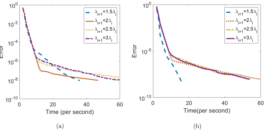
The penalty parameters λe and {λi}ni=1 play an important rule for the convex decom-position to be successful. We learn them through numerical experimentation (see Figures 5 and 6) and set them respectively to
(a) (b)
Figure 5: Learning turning parameter λe for two covariance estimation problems. Com-parison of the absolute errors produced by the algorithms based on CPU time for different choices of λe.
It can be seen from Figure 5 that with the addition of the ridge penalty term λe
2 kEk 2 F the algorithm clearly outperforms its unmodified counterpart in terms of CPU time for any fixed number of iterations. Indeed, when the model becomes more dense, SSONA is more effective to recover the network structure.
(a) (b)
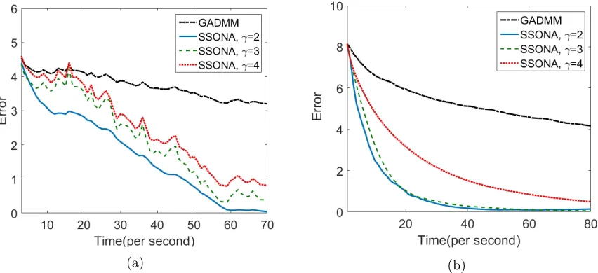
Next, we conduct experiments to assess the performance of the developed multi-block ADMM algorithm (SSONA) vis-a-vis the GADMM for solving two covariance graph esti-mation problems of dimension 1000 in the presence of noise. Figure 7 depicts the absolute error of the objective function for different choices of the regularization parameterγ of the augmented Lagrangian and that of the dense noisy component λe; note that the latter is key for the convergence of the proposed algorithm.
(a) (b)
Figure 7: Comparison of the absolute errors produced by the algorithms based on CPU time for different choices of γ.
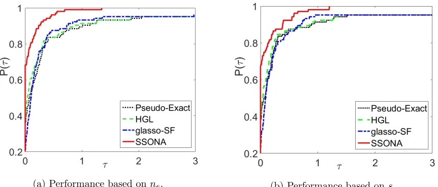
We define the following two performance measures, as proposed in Tan et al. (2014):
• Number of correctly estimated edges, ne : X
j<j0
1{|Θˆ|>1e−4 and|Θjj0|6=0}
.
• Sum of squared errors, se:
X
j<j0
|Θˆjj0−Θjj0| 2
.
The experiment is repeated ten times and the average number of correctly estimated edges, ne and sum of squared errors, se are considered for comparison. We have used the
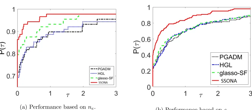
the percentage of the test problems that were successfully solved by each method (robust-ness). The performance profiles of the considered algorithms in log2 scale are depicted in Figures 8,9 and 10.
(a) Performance based onne. (b) Performance based onse.
Figure 8: Performance profiles of CovSel, HGL, glasso-SF and SSONA
(a) Performance based onne. (b) Performance based onse.
Figure 9: Performance profiles of Pseudo-Exact, HGL, glasso-SF and SSONA.
(a) Performance based onne. (b) Performance based ons e.
Figure 10: Performance profiles of PGADM, HGL, glasso-SF and SSONA.
ne and minimum value of estimation loss se. Further, the performance index of SSONA grows up rapidly in comparison with the other considered algorithms. The latter implies that whenever SSONA is not the best algorithm, its performance index is close to the index of the best one.
4.1.1 Experiments on structured graphical models
In this section, we present numerical results on structured graphical models to demonstrate the efficiency of SSONA. We compare the behavior of SSONA for a fixed value of p= 100 with a lasso version of our algorithm. Results provided in Figures 11, 12, 13 and 14 indicate the efficiency of algorithm 1 on structured graphical models. These results also show how the structure of the network returned by the two algorithms changes with growingm (note that λi and ˆλi are kept fixed for each value of m). It can be easily seen from these figures (comparing Row I and II) that SSONA is less sensitive to the number of samples and shows a better approximation of the network structure even for small sample sizes.
4.2 Classification and clustering accuracy based on SSONA
In this section, we evaluate the efficiency of SSONA on real data sets in recovering complex structured sparsity patterns and subsequently evaluate them on a classification task. The two data sets deal with applications in cancer genomic and document classification.
4.2.1 SSONA for Gene Selection Task
Classification with a sparsity constraint has become a standard tool in applications involv-ing Omics data, due to the large number of available features and the small number of samples. The data set under study considers gene expression profiles of lung cancer tumors. Specifically, the data2 consist of gene expression profiles of 12,626 genes for 197 lung tissue
(a) Graphical lasso.
(b) SSONA.
(c) Ground truth.
(d) Graphical lasso. (e) SSONA.
(f) Ground truth.
Figure 11: Simulation for the Gaussian graphical model. Row I: Results for p = 100 and m= 200. Row II: Results for p= 100 andm= 100.
(a) Graphical lasso. (b) SSONA.
(c) Ground truth.
(d) Graphical lasso. (e) SSONA.
(f) Ground truth.
Figure 12: Simulation for the Covariance graph model. Row I: Results for p= 100 andm= 200. Row II: Results forp= 100 and m= 100.
Method
Average
classifica-tion accuracy
Average number of
genes selected Group lasso (Yuan and Lin, 2007) 0.815(0.046) 69.11(3.23) Group lasso with overlap (Obozinski et al., 2011) 0.834(0.035) 57.30(2.71) SSONA (4 structured matrices) 0.807(0.028) 61.44(2.80) SSONA (6 structured matrices) 0.839(0.022) 56.111(2.100)
Table 1: Experimental results on lung cancer data over 10 replications (the standard devi-ations are reported in parentheses).
(a) Graphical lasso. (b) SSONA.
(c) Ground truth.
(d) Graphical lasso. (e) SSONA.
(f) Ground truth.
Figure 13: Simulation for the Gaussian graphical model with 10 latent variables. Row I: Results forp= 100 andm= 200. Row II: Results forp= 100 and m= 100.
In our experiments, SSONA selects the least number of genes and achieves the smallest standard deviation of average number of genes without any priori knowledge. Due to the different number of randomly selected genes, the average number of gene sometimes will be a non-integer.
4.2.2 SSONA for Document Classification Task
The next example involves a data set 3 containing 1427 documents with a corpus of size 17785 words. We randomly partition the data into 999 training, 214 validation and 214 test examples, corresponding to a 70/15/15 split (Rao et al., 2016). We first train a Latent Dirichlet Allocation based topics model (Blei et al., 2003) to assign the words to 100 ”top-ics”. These correspond to our groups, and since a single word can be assigned to multiple topics, the groups overlap. We then train a lasso logistic model using as outcome variable indicating whether the document discusses atheism or not , together with an overlapping group lasso and a SSON based lasso model where the tuning parameters are selected based on cross validation. Table 2 shows that the variants of the SSON yield almost the same misclassification rate compared to the other two methods, while it does not require a priori knowledge of group structures.
(a) Graphical lasso. (b) SSONA. (c) Ground truth.
(d) Graphical lasso. (e) SSONA. (f) Ground truth.
Figure 14: Simulation for the binary Ising Markov random field. Row I: Results for p= 100 and
m= 200. Row II: Results forp= 100 andm= 100.
Method Misclassification Rate
Group lasso (Yuan and Lin, 2007) 0.445 Group lasso with overlap (Obozinski et al., 2011) 0.390 SSONA (5 structured matrices) 0.435 SSONA (6 structured matrices) 0.421 SSONA (7 structured matrices) 0.401
Table 2: Misclassification rate on the test set for document classification.
4.2.3 SSONA for structured subspace clustering
Our last example focuses on data clustering. The data come from multiple low-dimensional linear or affine subspaces embedded in a high-dimensional space. Our method is based on (11), wherein each point in a union of subspaces has a representation with respect to a dictionary formed by all other data points. In general, finding such a representation is NP hard. We apply our subspace clustering algorithm to a structured data in the presence of noise. The segmentation of the data is obtained by applying SSONA to the adjacency matrix built from the data. Our method can handle noise and missing data and is effective to detect the clusters.
Ground Truth. Ground Truth+ Noise.
LRR (Liu et al., 2013). SSC (Elhamifar and Vidal, 2009).
SSONA.
Figure 15: Heatmap of different algorithms for detecting clusters in data.
4.3 Application to real data sets
Next, we use the SSON framework to analyze three data sets from molecular and social sci-ence domains. Although there is no known ground truth, the proposed framework recovers interesting patterns and highly interpretable structures.
Analysis of connectivity in the financial sector. We applied the SSON methodol-ogy to analyze connectivity in the financial sector. We use monthly stock returns data from August, 2001 to July, 2016 for three financial sectors, namely banks (BA), primary broker/dealers (PB), and insurance companies (INS). The data are obtained from the Uni-versity of Chicago’s Center for Research in Security Prices database (CRSP).
Figure 16: Average monthly return of firms in the three sectors- Bank, primary broker-dealer and insurance firms, in different 3-year rolling windows during 180 months. The figure shows diminished performance during the 2007-2009 crisis (time step : 80-100) and also clearly captures the strong recovery of stock performance starting in 2009.
Next, we estimate a measure of network connectivity for a sample of the 71 components of the SP100 index that were present during the entire 2001-16 period under consideration. Figure 17 depicts the network estimates of the transition (lead-lag) matrices using straight lasso VAR and SSONA based VAR for the January 2007 to Oct 2009 period. It can be seen that the lasso VAR estimates produce a more highly connected network, while the SSONA ones identify two more connected components. Both methods highlight the key role played by AIG and GS (Goldman Sachs), but the SSONA based network indicates that one dense connected component is centered around the former, while the other dense connected component around the latter. In summary, both methods capture the main connectivity patterns during the crisis period, but SSONA provides a more nuanced picture.
(a) SSONA VAR
(b) Lasso VAR
Figure 17: Networks estimate by SSONA and Lasso VAR during crisis period of Jan 2007 to Oct 2009.
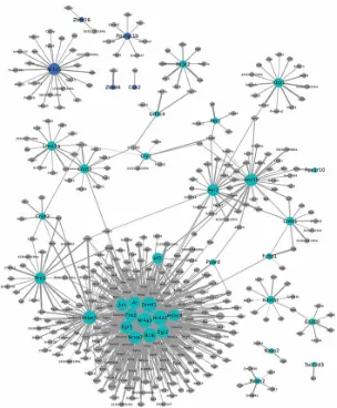
the adjacency matrix of the estimated network by using SSONA is depicted in Figure 18. It can be easily seen that there exist densely connected components in the network, a fact that the glasso algorithm (Friedman et al., 2008) fails to recover (see, Figure 19).
The network representation of subgraphs, with a cut-off value of 0.6, is given in Fig-ures 20, 21 and 22. We only plot the edges associated with the subgraphs to enhance the visual reading of densely correlated areas. An interesting result of applying SSONA on this data set is the clear separation between members of the Democratic and Republican parties, as expected (see, Figures 20, 21 and 22). Moreover, voting relationships within the two parties exhibit a clustering structure, which a closer inspection of the votes and subsequent analysis showed was mainly driven by the position of the House member on the ideological/political spectrum.
Z1+Z1>
Z2+Z2> Z3+Z3>
Z4+Z4>
Z5+Z5>
Z6+Z6>
Figure 18: Heatmap of the structured precision matrix Θ decomposed intoZ1+Z1>+· · ·+ Z6+Z6> in the House voting data, estimated by SSONA.
Figure 19: Heatmap of the inverse covariance matrix in the voting record of the U.S. House of Representatives, estimated by the graphical lasso method (Friedman et al., 2008).
Figure 20: Dense subgraphs identified by SSONA for the House voting data with an inclusion cutoff value of 0.6. Subfigures correspond to a densely connected area in Figure 18 for the symmetric structured matrix Z2+Z2>. The nodes represent House members, with red and green colored nodes corresponding to Republicans and Democrats, respectively. A blue line corresponds to an edge between two nodes.
associations between members of the same party and negative associations between members of opposite parties. Obviously, at the higher cutoff value the dependence structure between members of opposite parties becomes sparser.
Figure 21: Dense subgraphs identified by SSONA for the House voting data with an inclusion cutoff value of 0.6. Subfigures correspond to a densely connected area in Figure 18 for the symmetric structured matrix Z3+Z3>. The nodes represent House members, with red and green colored nodes corresponding to Republicans and Democrats, respectively. A blue line corresponds to an edge between two nodes.
Figure 21. However, in this instance, there is also a cluster of positive associations between Democrats.
In summary, SSONA provides deeper insights into relationships between House mem-bers, going beyond the obvious separation into two parties, according to their voting record.
Figure 22: Dense subgraph identified by SSONA for the House voting data with an inclusion cutoff value of 0.6. Subfigures corresponds to a densely connected area in Figure 18 for the symmetric structured matrix Z5+Z5>. The nodes represent House members, with red and blue node colors corresponding to Republicans and Democrats, respectively. A blue line corresponds to an edge between two nodes.
Z1+Z1> Z2+Z>
2 Z3+Z
>
3
Z4+Z4> Z5+Z5> Z6+Z
>
6
Figure 23: Heat map of the structured precision matrix Θ decomposed intoZ1+Z1>+· · ·+ Z6+Z6> in the breast cancer data set, estimated by SSONA.
Figure 24: Heatmap of the inverse covariance matrix in the breast cancer data sets, esti-mated from graphical lasso (Friedman et al., 2008).
genes are densely connected, which is not the case when employing the the graphical lasso algorithm (see, Figure 24). Therefore, SSONA can provide an intuitive explanation of the relationships among the genes in the breast cancer data set (see, Figure 25 and 26 for two examples). These genes connectivity in the tumor samples may indicate a relationship that is common to an important subset of cancers. Many other genes belong to this network, each indicating a potentially interesting interaction in cancer biology. We omit the full list of densely connected genes in our estimated network and provide a complete list in the on-line supplementary materials available in the first author’s homepage.
Figure 26: Network layout of grouped genes identified by SSONA for the breast cancer data set. Subfigure corresponds to a densely connected component in Figure 23 for the structured matrixZ6+Z6>.
5. Conclusion
In this paper, a new structured norm minimization method for solving multi-structure graphical model selection problems is proposed. Using the proposed SSON, we can efficiently and accurately recover the underlying network structure. Our method utilizes a class of sparse structured norms in order to achieve higher order accuracy in approximating the decomposition of the parameter matrix in Markov Random Field and Gaussian Covariance Graph models. We also provide a brief discussion of its application to regression and classification problems. Further, we introduce a linearized multi-block ADMM algorithm to solve the resulting optimization problem. The global convergence of the algorithm is established without any upper bound on the penalty parameter. We applied the proposed methodology to a number of real and synthetic data sets that establish its overall usefulness and superior performance to competing methods in the literature.
Acknowledgments
The authors would like to thank the Editor and three anonymous referees for many construc-tive comments and suggestions that improved significantly the structure and readability of the paper. This work was supported in part by NSF grants DMS-1545277, DMS-1632730, NIH grant 1R01-GM1140201A1 and by the UF Informatics Institute.
Appendix A. Update for Θ
1. The update for Θ1 in Algorithm 1 (step 2(a)) can be obtained by minimizing
trace( ˆΣΘ1)−log det Θ1+ γ
2kΘ1−( n X
i=1
Zik+Zik>+Ek+ 1 γΛ
k)k2 F,
with respect to Θ1 (note that the constraint Θ1 ∈ S in (6) is treated as an implicit constraint, due to the domain of definition of the log det function). This can be shown to have the solution
Θ1 = 1 2U
D+
r
D2+4 γI
UT,
whereU DUT stands for the eigen-decomposition ofPni=1Zik+Zik>+Ek+1γΛk−1 γΣ.ˆ 2. Update for Θ2in Step 2(a) of Algorithm 1 leads to the following optimization problem
minimize Θ3∈S
Φ(Θ2) = p X j=1 p X
j0=1
θjj0(XTX)jj0− m X i=1 p X j=1 log
1 + exp[θjj+ X
j06=j
θjj0xij0]
+ γ
2kΘ2−( n X
i=1
Zik+Zik>+Ek+ 1 γΛ
k)k2
F. (33)
We use a novel non-monotone version of the Barzilai-Borwein method (Barzilai and Borwein, 1988; Raydan, 1997; Fletcher, 2005; Ataee Tarzanagh et al., 2014) to solve (33). The details are given in Algorithm 2.
Algorithm 2 Non-monotone Barzilai Borwein Method for solving (33) Initialize The parameters:
(a) Θ0=I, Θ1= 2Θ0,α1 = 1 and t0= 10. (b) A positive sequence{ηt} satisfying P∞
k=1ηt=η <∞. (c) Constantsσ >0, >0, andν ∈(0,1).
Iterate Until the stopping criterion kΘ
t−Θt−1k2 F
kΘt−1k2 F
≤is met:
1. Gt=−αt∇Φ(Θt).
2. Setρ= 1. 3. If t > t0,then
While kΦ(Θt+ρtGt)kF ≤Φ(Θt) +ηt−σρ2αt2kGtk2F,do
Setρ=νρ; EndWhile EndIf
4. Define ρt=ρ and Θt+1 = Θt+ρtGt.
5. Define αt+1= trace
3. To update Θ3 in step 2(a), using (11), we have that
minimize Θ3
1
2kΘ3−Σˆk 2 F +
γ 2kΘ3−
Xn i=1
Zik+Zik>+Ek+ 1 γΛ
kk2 F
= 1
1 +γ( ˆΣ +γ( n X
i=1
Zik+Zik>+Ek) + Λk)
+ whereV+=U†D+U† such that
U DU = U† U‡
D+ 0
0 D−
U†
U‡
,
is the eigen-decomposition of the matrixV , andD+ andD− are the nonnegative and
negative eigenvalues of V.
Appendix B. Convergence Analysis
Before establishing the main result on global convergence of the proposed ADMM algorithm, we provide the necessary definitions used in the proofs (for more details see Bolte et al. (2014)):
Definition 11 (Kurdyka- Lojasiewicz property).
The functionf is said to have the Kurdyka- Lojasiewicz (K-L) property at pointZ0, if there
exist c1 >0, c2 >0 and φ∈Γc2 such that for all
Z ∈B(Z0, c1)∩ {Z :f(Z0)< f(Z)< f(Z0) +c2},
the following inequality holds
φ0 f(Z)−f(Z0)dist 0, ∂f(Z)≥1, where Γc2 stands for the class of functionsφ: [0, c2]→R
+ with the properties:
(i) φ is continuous on[0, c2); (ii) φ is smooth concave on (0, c2);
(iii) φ(0) = 0, ∇φ(s)>0, ∀ s∈(0, c2).
Definition 12 (Semi-algebraic sets and functions).
(i) A subsetC∈Rn×n is semi-algebraic, if there exists a finite number of real polynomial
functions hij,sij :Rn×n→R such that
C=∪pi=1¯ ∩qj=1¯ {Z ∈Rn×n: gij(Z) = 0 and sij(Z)<0}.
(ii) A function h:Rn×n→(−∞,+∞]is called semi-algebraic, if its graph
is a semi-algebraic set in Rn×n+1.
Definition 13 (Sub-analytic sets and functions).
(i) A subset C ∈ Rn×n is sub-analytic, if there exists a finite number of real analytic
functions hij,sij :Rn×n→R such that
C =∪pi=1¯ ∩qj=1¯ {Z ∈Rd:gij(Z) = 0 and sij(Z)<0}.
(ii) A function h: Rn×n→(−∞,+∞] is called sub-analytic, if its graph
G(h) :={(Z, y)∈Rn×n+1 :h(Z) =y}
is a sub-analytic set in Rn×n+1.
It can be easily seen that both real analytic and semi-algebraic functions are sub-analytic. In general, the sum of two sub-analytic functions is not necessarily sub-sub-analytic. However, it is easy to show that for two sub-analytic functions, if at least one function maps bounded sets to bounded sets, then their sum is also sub-analytic (Bolte et al., 2014).
Remark 14 Eachfiin (19)is a convex semi-algebraic function (see, example 5.3 in (Bolte
et al., 2014)), while the loss functionG in (6),(9),(11),(13), and (18)is sub-analytic (even analytic). Since each function fi maps bounded sets to bounded sets, we can conclude that
the augmented Lagrangian function
Lγ(Θ, Z1, . . . , Zn, E; Λ) = G(X,Θ) +f1(Z1) +· · ·+fn(Zn) +fe(E)
− hΛ,Θ−
n X
i=1
Zi+Zi>−Ei
+ γ 2kΘ−
n X
i=1
Zi+Zi>−Ek2F,
which is the summation of sub-analytic functions is itself sub-analytic. All sub-analytic functions which are continuous over their domain satisfy a K-L inequality, as well as some, but not all, convex functions (see Bolte et al., 2014 for details and a counterexample). Therefore, the augmented Lagrangian function Lγ satisfies the K-L property.
Next, we establish a series of lemmas used in the proof of Theorem 10.
Lemma 15 Let Uk := (Θk, Z1k, . . . , Znk, Ek; Λk) be a sequence generated by Algorithm 1, then there exists a positive constantϑ such that
Lγ(Uk+1) ≤ Lγ(Uk)−
ϑ
2
kΘk−Θk+1kF
+
n
X
i=1
kZik−Zik+1kF+kEk−Ek+1kF+kΛk−Λk+1kF
Proof. Using the first-order optimality conditions for (21) and the convexity ofG(X,Θ), we obtain
0 =
Θk−Θk+1,∇G(X,Θk+1)−Λk+γ(Θk+1−
n X
i=1
Zik+Zik>−Ek)
≤ G(X,Θk)− G(X,Θk+1)− hΘk−Θk+1,Λki
+ γhΘk−Θk+1,Θk+1−
n X
i=1
Zik+Zik>−Eki
= G(X,Θk)− hΘk,Λki+γ 2
n X
i=1
kΘk−
n X
i=1
Zik+Zik>−Ekk2 F −
γ 2kΘ
k−Θk+1k2 F
− G(X,Θk+1)− hΘk+1,Λki+ γ 2kΘ
k+1− n X
i=1
Zik+Zik>−Ekk2F
= Lγ(Uk)− Lγ(Θk+1, Z1k, . . . , Znk, Ek; Λk)−γ
2kΘ
k−Θk+1k2
F, (35) where the second equality follows from the fact that
(u1−u2)T(u3−u1) = 1 2
ku2−u3k2F − ku1−u2k2F − ku1−u3k2F
.
Using (22), (23) and Lemma 7, we have that
Lγ(Θk+1, Z1k, Z2k, . . . , Ek; Λk) − Lγ(Θk+1, Z1k+1, Z2k, . . . , Ek; Λk)
− (γ%−LH1) 2 kZ
k
1 −Z1k+1k2F
≥ 0,
Lγ(Θk+1, . . . , Zik+1−1, Zik, . . . , Ek; Λk) − Lγ(Θk+1, . . . , Zik+1, Zi+1k , . . . , Ek; Λk)
− (γ%−LHi)
2 kZ k
i −Zik+1k2F
≥ 0, i= 2, . . . , n, (36)
where LHi is a Lipschitz constant of the gradient∇Hi(Zi), and % ≥
LHi
γ , (i= 1, . . . , n) is a proximal parameter.
Following the same steps as (35), we have that
Lγ(Θk, Z1k+1, . . . , Znk+1, Ek; Λk) − Lγ(Θk+1, Z1k+1, . . . , Znk+1, Ek+1; Λk)
− γ
2kE
k−Ek+1k2 F
≥ 0, (37)
and
Lγ(Θk+1, Z1k+1, . . . , Znk+1, Ek+1; Λk) − Lγ(Θk+1, Z1k+1, . . . , Znk+1, Ek+1; Λk+1)
− λ
2 e γ kE
k−Ek+1k2 F
Let
ˆ
γ := max(γ%−LH1, . . . , γ%−LHn), γ¯:=
γ2−2λ2e γ(1 +λ2
e)
, ϑ:= max(ˆγ,¯γ, γ).
Then, using (35)– (38), and γ ≥√2λe, we have
Lγ(Uk)− Lγ(Uk+1)≥ γ
2kΘ
k−Θk+1k2 F
+ ˆγ 2
n X
i=1
kZik−Zik+1k2 F +
γ2−2λ2e 2γ kE
k−Ek+1k2 F,
= γ 2kΘ
k−Θk+1k2 F + ˆ γ 2 n X i=1
kZik−Zik+1k2F +¯γ 2kE
k−Ek+1k2 F +
λ2e¯γ 2 kE
k−Ek+1k2 F,
= γ 2kΘ
k−Θk+1k2 F + ˆ γ 2 n X i=1
kZik−Zik+1k2 F +
¯ γ 2
kEk−Ek+1k2
F +kΛk−Λk+1k2F
,
≥ ϑ
2
kΘk−Θk+1k2F + n X
i=1
kZik−Zik+1k2F +kEk−Ek+1k2F +kΛk−Λk+1k2F.
2
Lemma 16 Let Uk = (Θk, Z1k, . . . Xnk, Ek,Λk) be a sequence generated by Algorithm 1. Then, there exists a subsequence Uks of {Uk}, such that
lim
s→∞G(X,Θ
ks) =g(Θ∗), lim
s→∞fi(Z
ks
i ) =fi(Z
∗
i), slim→∞fe(Eiks) =fe(E
∗
i),
where
lim s→∞U
ks = (Θ∗, Z∗
1, . . . , Z
∗
n, E
∗
,Λ∗).
Proof. Let Υk+1 = Θk+1−Pni=1Zik+1+Zik+1>−Ek+1. Using the quadratic function fe(E) = λ2ekEk2F, we have that
fe(Ek+1−Υk+1) = λe
2 kE
k+1−Υk+1k2 F = λe
2 kE
k+1k2−λ
ehEk+1,Υk+1i+ λe
2 kΥ k+1k2
F. (39) Using (39) and the fact that each functionfi is lower bounded, there existsL, such that
Lγ(Uk+1) = G(X,Θk+1) +f1(Z1k+1) +. . . fn(Znk+1) +λe 2 kE
k+1−Υk+1k2 F + γ−λe
2 kΥ k+1k2
F ≥g+f1+· · ·+fn≥ L, (40)
ϑ 2
K X
k=0
kΘk−Θk+1k2F + n X
i=1
kZik−Zik+1k2F + kEk−Ek+1k2F +kΛk−Λk+1k2F
≤ Lγ(U0)− L. (41)
Lemma 15 together with (41) shows that Lγ(Uk) converges to Lγ(U∗). Note that (41) and the coerciveness of G(X,Θ) and fi (i = 1, . . . , n) imply that {(Θk, Z1k, . . . , Znk)} is a bounded sequence. This together with the updating formula of Λk+1 and (41) yield the boundedness ofEk+1. Moreover, the fact that Λk =−λeEk, gives the boundedness of Λk, which implies that the entire sequence {Uk} is a bounded one. Therefore, there exists a subsequence
Uks = (Θks, Zks
1 , . . . , Z ks
n , Eks; Λks), s= 0,1, . . .
such thatUks →U∗ ass→ ∞.
Now, using the fact that G(X,Θ),fi(Zi) (i= 1, . . . , n) and fe(E) are continuous func-tions, we have that
lim
s→∞G(X,Θ
ks) =g(Θ∗), lim
s→∞fi(Z
kq
i ) =fi(Z
∗
i), slim→∞fe(E kq
i ) =fe(E
∗
i).
2
Lemma 17 Algorithm 1 either stops at a stationary point of the problem (19) or generates an infinite sequence{Uk}, so that any limit point of{Uk}is a critical point ofLγ(Uk) (19).
Proof. From the definition of the augmented Lagrangian function in (19), we have that
∇G(X,Θk+1)−Λk+1+γΥk+1=∇ΘLγ(Uk+1), ∂fi(Zik+1)−Λ
k+1−Λk+1>−γ(Υk+1+ Υk+1>)∈∂
ZiLγ(U
k+1), i= 1, . . . , n, λeEk+1+ Λk+1−γΥk+1=∇ELγ(Uk+1),
γΥk+1 =−∇ΛLγ(Uk+1), (42)
where Υk+1 = Θk+1−Pni=1Zik+1+Zik+1>−Ek+1.
∇G(X,Θk+1)−Λk+1 = γΘk+1−Θk
+ n X
i=1
Zik−Zik+1+ (Zik−Zik+1)>+Ek−Ek+1
∂f1(Z1k+1)−Λ
k+1−Λk+1> = γ%(Zk
1 −Z1k+1) +γ
Θk+1−Θk
+ (Θk+1−Θk)>+ n X
i=1
Zik−Zik+1 (43)
+ (Zik−Zik+1)>+Ek−Ek+1+ (Ek−Ek+1)> ∂fi(Zik+1)−Λk+1−Λk+1
>
= γ%(Zik−Zik+1)
+ γΘk+1−Θk+ (Θk+1−Θk)>
+ n X
j=i
Zik−Zik+1+ (Zik−Zik+1)>
+ Ek−Ek+1+ (Ek−Ek+1)> i= 2, . . . , n,
λeEk+1 + Λk+1= 0. (44)
Combining (42), (43), and the updating formula of Λk+1, we have that
(~k+1Θ ,~ k+1
1 , . . . ,~k+1n ,~k+1E ,~ k+1
Λ )∈∂Lγ(Uk+1), (45) where
~k+1Θ := Λk−Λk+1+γ
Θk+1−Θk+ n X
i=1
Zik−Zik+1+ (Zik−Zik+1)>+Ek−Ek+1
~k+1Z1 := Λ
k−Λk+1+ (Λk−Λk+1)>
+γ%(Z1k−Z1k+1) + γ
Θk+1−Θk+ (Θk+1−Θk)>+ n X
i=1
Zik−Zik+1+ (Zik−Zik+1)>
+ Ek−Ek+1+ (Ek−Ek+1)>
~k+1Zi := Λk−Λk+1+ (Λk−Λk+1)>+γ%(Zik−Zik+1)
+ γ
Θk+1−Θk+ (Θk+1−Θk)>+ n X
j=i
Zik−Zik+1+ (Zik−Zik+1)>
+ Ek−Ek+1+ (Ek−Ek+1)>, i= 2, . . . , n,
~k+1E := Λ
k−Λk+1,
~k+1Λ :=
1 γ(Λ