Online Tensor Methods for Learning Latent Variable Models

Online Tensor Methods for Learning Latent Variable Models

Furong Huang furongh@uci.edu

U. N. Niranjan un.niranjan@uci.edu

Mohammad Umar Hakeem mhakeem@uci.edu

Animashree Anandkumar a.anandkumar@uci.edu

Electrical Engineering and Computer Science Dept. University of California, Irvine

Irvine, USA 92697, USA

Editor:David Blei

Abstract

We introduce an online tensor decomposition based approach for two latent variable mod-eling problems namely, (1) community detection, in which we learn the latent communities that the social actors in social networks belong to, and (2) topic modeling, in which we infer hidden topics of text articles. We consider decomposition of moment tensors using stochastic gradient descent. We conduct optimization of multilinear operations in SGD and avoid directly forming the tensors, to save computational and storage costs. We present optimized algorithm in two platforms. Our GPU-based implementation exploits the par-allelism of SIMD architectures to allow for maximum speed-up by a careful optimization of storage and data transfer, whereas our CPU-based implementation uses efficient sparse matrix computations and is suitable for large sparse data sets. For the community detec-tion problem, we demonstrate accuracy and computadetec-tional efficiency on Facebook, Yelp and DBLP data sets, and for the topic modeling problem, we also demonstrate good per-formance on the New York Times data set. We compare our results to the state-of-the-art algorithms such as the variational method, and report a gain of accuracy and a gain of several orders of magnitude in the execution time.

Keywords: mixed membership stochastic blockmodel, topic modeling, tensor method, stochastic gradient descent, parallel implementation, large datasets

1. Introduction

1.1 Summary of Contributions

We consider two problems: (1) community detection (wherein we compute the decompo-sition of a tensor which relates to the count of 3-stars in a graph) and (2) topic modeling (wherein we consider the tensor related to co-occurrence of triplets of words in documents); decomposition of the these tensors allows us to learn the hidden communities and topics from observed data.

Community detection: We recover hidden communities in several real datasets with high accuracy. When ground-truth communities are available, we propose a new error score based on the hypothesis testing methodology involving p-values and false discovery rates (Strimmer, 2008) to validate our results. The use of p-values eliminates the need to carefully tune the number of communities output by our algorithm, and hence, we obtain a flexible trade-off between the fraction of communities recovered and their estimation accuracy. We find that our method has very good accuracy on a range of network datasets: Facebook, Yelp and DBLP. We summarize the datasets used in this paper in Table 6. To get an idea of our running times, let us consider the larger DBLP collaborative data set for a moment. It consists of 16 million edges, one million nodes and 250 communities. We obtain an error of 10% and the method runs in about two minutes, excluding the 80 minutes taken to read the edge data from files stored on the hard disk and converting it to sparse matrix format.

Compared to the state-of-the-art method for learning MMSB models using the stochas-tic variational inference algorithm of (Gopalan et al., 2012), we obtain several orders of magnitude speed-up in the running time on multiple real datasets. This is because our method consists of efficient matrix operations which are embarrassingly parallel. Matrix operations are carried out in the sparse format which is efficient especially for social net-work settings involving large sparse graphs. Moreover, our code is flexible to run on a range of graphs such as directed, undirected and bipartite graphs, while the code of (Gopalan et al., 2012) is designed for homophilic networks, and cannot handle bipartite graphs in its present format. Note that bipartite networks occur in the recommendation setting such as the Yelp data set. Additionally, the variational implementation in (Gopalan et al., 2012) assumes a homogeneous connectivity model, where any pair of communities connect with the same probability and the probability of intra-community connectivity is also fixed. Our framework does not suffer from this restriction. We also provide arguments to show that the Normalized Mutual Information (NMI) and other scores, previously used for evaluating the recovery of overlapping community, can underestimate the errors.

Topic modeling: We also employ the tensor method for topic-modeling, and there are many similarities between the topic and community settings. For instance, each document has multiple topics, while in the network setting, each node has membership in multiple communities. The words in a document are generated based on the latent topics in the document, and similarly, edges are generated based on the community memberships of the node pairs. The tensor method is even faster for topic modeling, since the word vocabulary size is typically much smaller than the size of real-world networks. We learn interesting hidden topics in New York Times corpus from UCI bag-of-words data set1 with around 100,000 words and 300,000 documents in about two minutes. We present the important

words for recovered topics, as well as interpret “bridging” words, which occur in many topics.

Implementations: We present two implementations, viz., a GPU-based implementation which exploits the parallelism of SIMD architectures and a CPU-based implementation for larger datasets, where the GPU memory does not suffice. We discuss various aspects involved such as implicit manipulation of tensors since explicitly forming tensors would be unwieldy for large networks, optimizing for communication bottlenecks in a parallel deployment, the need for sparse matrix and vector operations since real world networks tend to be sparse, and a careful statistical approach to validating the results, when ground truth is available.

1.2 Related work

This paper builds on the recent works of Anandkumar et al (Anandkumar et al., 2012, 2013b) which establishes the correctness of tensor-based approaches for learning MMSB (Airoldi et al., 2008) models and other latent variable models. While, the earlier works provided a theoretical analysis of the method, the current paper considers a careful implementation of the method. Moreover, there are a number of algorithmic improvements in this paper. For instance, while (Anandkumar et al., 2012, 2013b) consider tensor power iterations, based on batch data and deflations performed serially, here, we adopt a stochastic gradient descent approach for tensor decomposition, which provides the flexibility to trade-off sub-sampling with accuracy. Moreover, we use randomized methods for dimensionality reduction in the preprocessing stage of our method which enables us to scale our method to graphs with millions of nodes.

There are other known methods for learning the stochastic block model based on tech-niques such as spectral clustering (McSherry, 2001) and convex optimization (Chen et al., 2012). However, these methods are not applicable for learning overlapping communities. We note that learning the mixed membership model can be reduced to a matrix factor-ization problem (Zhang and Yeung, 2012). While collaborative filtering techniques such as (Mnih and Salakhutdinov, 2007; Salakhutdinov and Mnih, 2008) focus on matrix factor-ization and the prediction accuracy of recommendations on an unseen test set, we recover the underlying latent communities, which helps with the interpretability and the statistical model can be employed for other tasks.

Although there have been other fast implementations for community detection be-fore (Soman and Narang, 2011; Lancichinetti and Fortunato, 2009), these methods are not statistical and do not yield descriptive statistics such as bridging nodes (Nepusz et al., 2008), and cannot perform predictive tasks such as link classification which are the main strengths of the MMSB model. With the implementation of our tensor-based approach, we record huge speed-ups compared to existing approaches for learning the MMSB model.

tensor decompositions through stochastic updates. This is a crucial departure from other works on tensor decompositions on GPUs (Ballard et al., 2011; Schatz et al., 2013), where the tensor needs to be stored and manipulated directly.

2. Tensor Forms for Topic and Community Models

In this section, we briefly recap the topic and community models, as well as the tensor forms for their exact moments, derived in (Anandkumar et al., 2012, 2013b).

2.1 Topic Modeling

In topic modeling, a document is viewed as a bag of words. Each document has a latent set of topics, andh= (h1, h2, . . . , hk) represents the proportions ofktopics in a given document. Given the topics h, the words are independently drawn and are exchangeable, and hence, the term “bag of words” model. We represent the words in the document byd-dimensional random vectors x1, x2, . . . xl ∈Rd, where xi are coordinate basis vectors inRd and dis the

size of the word vocabulary. Conditioned onh, the words in a document satisfy E[xi|h] =

µh, where µ := [µ1, . . . , µk] is the topic-word matrix. And thus µj is the topic vector

satisfying µj = Pr (xi|hj), ∀j ∈ [k]. Under the Latent Dirichlet Allocation (LDA) topic model (Blei, 2012), h is drawn from a Dirichlet distribution with concentration parameter

vectorα = [α1, . . . , αk]. In other words, for each document u, hu iid∼ Dir(α), ∀u ∈[n] with parameter vectorα∈_Rk

+. We define the Dirichlet concentration (mixing) parameter

α0:= X

i∈[k] αi.

The Dirichlet distribution allows us to specify the extent of overlap among the topics by controlling for sparsity in topic density function. A larger α0 results in more overlapped

(mixed) topics. A special case ofα0= 0 is the single topic model.

Due to exchangeability, the order of the words does not matter, and it suffices to consider the frequency vector for each document, which counts the number of occurrences of each word in a document. Let ct := (c1,t, c2,t, . . . , cd,t) ∈Rd denote the frequency vector for tth

We consider the first three order empirical moments, given by

M₁Top:= 1

n

n X

t=1

ct (1)

M₂Top:= α0+ 1

n

n X

t=1

(ct⊗ct−diag (ct))−α0M Top

1 ⊗M

Top

1 (2)

M₃Top:= (α0+ 1)(α0+ 2) 2n

n X

t=1 

ct⊗ct⊗ct− d X i=1 d X j=1

ci,tcj,t(ei⊗ei⊗ej)

− d X i=1 d X j=1

ci,tcj,t(ei⊗ej⊗ei)− d X i=1 d X j=1

ci,tcj,t(ei⊗ej⊗ej) + 2 d X

i=1

ci,t(ei⊗ei⊗ei) 



−α0(α0+ 1) 2n n X t=1 d X i=1

ci,t(ei⊗ei⊗M

Top

1 ) +

d X

i=1

ci,t(ei⊗M

Top

1 ⊗ei) +

d X

i=1

ci,t(M

Top

1 ⊗ei⊗ei)

!

+α2₀M₁Top⊗M₁Top⊗M₁Top. (3)

We recall Theorem 3.5 of (Anandkumar et al., 2012):

Lemma 1 The exact moments can be factorized as

E[M1Top] = k X

i=1 αi

α0µi (4)

E[M2Top] = k X

i=1 αi

α0µi⊗µi (5)

E[M3Top] = k X

i=1 αi α0

µi⊗µi⊗µi. (6)

where µ= [µ1, . . . , µk] and µi = Pr (xt|h=i), ∀t∈[l]. In other words, µ is the topic-word matrix.

From the Lemma 1, we observe that the first three moments of a LDA topic model have a simple form involving the topic-word matrix µand Dirichlet parameters αi. In

(Anand-kumar et al., 2012), it is shown that these parameters can be recovered under a weak non-degeneracy assumption. We will employ tensor decomposition techniques to learn the parameters.

2.2 Mixed Membership Model

In the mixed membership stochastic block model (MMSB), introduced by (Airoldi et al., 2008), the edges in a social network are related to the hidden communities of the nodes. A batch tensor decomposition technique for learning MMSB was derived in (Anandkumar et al., 2013b).

Let n denote the number of nodes, k the number of communities and G ∈ Rn×n the

vectorπi ∈Rk, which is a latent variable, and the vectors are contained in a simplex, i.e.,

X

i∈[k]

πu(i) = 1, ∀u∈[n]

where the notation [n] denotes the set {1, . . . , n}. Membership vectors are sampled from

the Dirichlet distributionπu iid∼Dir(α), ∀u∈[n] with parameter vectorα∈Rk+whereα0 := P

i∈[k]αi. As in the topic modeling setting, the Dirichlet distribution allows us to specify

the extent of overlap among the communities by controlling for sparsity in community membership vectors. A larger α0 results in more overlapped (mixed) memberships. A special case of α0 = 0 is the stochastic block model (Anandkumar et al., 2013b).

The community connectivity matrix is denoted byP ∈[0,1]k×k whereP(a, b) measures the connectivity between communitiesaand b,∀a, b∈[k]. We model the adjacency matrix entries as either of the two settings given below:

Bernoulli model: This models a network with unweighted edges. It is used for Facebook and DBLP datasets in Section 6 in our experiments.

Gij iid∼Ber(π_i>P πj), ∀i, j∈[n].

Poisson model (Karrer and Newman, 2011): This models a network with weighted edges. It is used for the Yelp data set in Section 6 to incorporate the review ratings.

Gij iid

∼Poi(π_i>P πj), ∀i, j∈[n].

The tensor decomposition approach involves up to third order moments, computed from the observed network. In order to compute the moments, we partition the nodes randomly into sets X, A, B, C. Let FA := Π>AP>, FB := Π>BP>, FC := Π>CP> (where P is the

community connectivity matrix and Π is the membership matrix) and ˆα := α1

α0, . . . ,

αk α0

denote the normalized Dirichlet concentration parameter. We define pairs over Y1 and Y2

as Pairs(Y1, Y2) :=G>X,Y1 ⊗G

>

X,Y2. Define the following matrices

ZB:= Pairs (A, C) (Pairs (B, C))†, (7)

ZC := Pairs (A, B) (Pairs (C, B))†. (8)

We consider the first three empirical moments, given by

M1Com:=

1

nX

X

x∈X

G>_x,A (9)

M2Com:=

α0+ 1 nX

X

x∈X

ZCG>x,CGx,BZB>−α0

M1ComM1Com

>

(10)

M3Com:= (α0+ 1)(α0+ 2) 2nX

X

x∈X h

G>_x,A⊗ZBG>_x,B⊗ZCG>_x,C i

+α₀2M1Com⊗M1Com⊗M1Com

− α0(α0+ 1) 2nX

X

x∈X h

G>_x,A⊗ZBG>x,B ⊗M1Com+G>x,A⊗M1Com⊗ZCG>x,C (11)

+M1Com⊗ZBG>x,B⊗ZCG>x,C i

We now recap Proposition 2.2 of (Anandkumar et al., 2013a) which provides the form of these moments under expectation.

Lemma 2 The exact moments can be factorized as

E[M1Com|ΠA,ΠB,ΠC] := X

i∈[k]

ˆ

αi(FA)i (13)

E[M2Com|ΠA,ΠB,ΠC] := X

i∈[k]

ˆ

αi(FA)i⊗(FA)i (14)

E[M3Com|ΠA,ΠB,ΠC] := X

i∈[k]

ˆ

αi(FA)i⊗(FA)i⊗(FA)i (15)

where ⊗ denotes the Kronecker product and(FA)i corresponds to the ith column of FA.

We observe that the moment forms above for the MMSB model have a similar form as the moments of the topic model in the previous section. Thus, we can employ a unified framework for both topic and community modeling involving decomposition of the third order moment tensorsM₃Top andM₃Com. Second order momentsM₂Topand M₂Com are used forpreprocessing of the data (i.e., whitening, which is introduced in detail in Section 3.1). For the sake of the simplicity of the notation, in the rest of the paper, we will use M2 to

denote empirical second order moments for bothM₂Topin topic modeling setting, andM₂Com

in the mixed membership model setting. Similarly, we will useM3 to denote empirical third order moments for bothM₃Top andM₃Com.

3. Learning using Third Order Moment

Our learning algorithm uses up to the third-order moment to estimate the topic word matrixµor the community membership matrix Π. First, we obtain co-occurrence of triplet words or subgraph counts (implicitly). Then, we perform preprocessing using second order moment M2. Then we perform tensor decomposition efficiently using stochastic gradient descent (Kushner and Yin, 2003) on M3. We note that, in our implementation of the

algorithm on the Graphics Processing Unit (GPU), linear algebraic operations are extremely fast. We also implement our algorithm on the CPU for large datasets which exceed the memory capacity of GPU and use sparse matrix operations which results in large gains in terms of both the memory and the running time requirements. The overall approach is summarized in Algorithm 1.

3.1 Dimensionality Reduction and Whitening

Whitening step utilizes linear algebraic manipulations to make the tensor symmetric and orthogonal (in expectation). Moreover, it leads to dimensionality reduction since it (im-plicitly) reduces tensor M3 of size O(n3) to a tensor of size k3, where k is the number of communities. Typically we havekn. The whitening step also converts the tensorM3 to a symmetric orthogonal tensor. The whitening matrix W ∈_RnA×k _{satisfies W}>_M

2W =I.

Algorithm 1 Overall approach for learning latent variable models via a moment-based approach.

Input: Observed data: social network graph or document samples.

Output: Learned latent variable model and infer hidden attributes.

1: Estimate the third order moments tensor M3 (implicitly). The tensor is not formed explicitly as we break down the tensor operations into vector and matrix operations. 2: Whiten the data, via SVD of M2, to reduce dimensionality via symmetrization and

orthogonalization. The third order momentsM3 are whitened asT.

3: Use stochastic gradient descent to estimate spectrum of whitened (implicit) tensorT. 4: Apply post-processing to obtain the topic-word matrix or the community memberships.

5: If ground truth is known, validate the results using various evaluation measures.

result in an orthogonal tensor. We use multilinear operations to get an orthogonal tensor T :=M3(W, W, W).

The whitening matrixW is computed via truncatedk−svd of the second order moments.

W =UM2Σ

−1/2 M2 ,

where UM2 and ΣM2 = diag(σM2,1, . . . , σM2,k) are the top k singular vectors and singular

values ofM2 respectively. We then perform multilinear transformations on the triplet data using the whitening matrix. The whitened data is thus

y_At := W, ct

,

yt_B:= W, ct

,

y_Ct :=W, ct,

for the topic modeling, wheret denotes the index of the documents. Note thaty_At,y_Bt and

y_Ct ∈ Rk. Implicitly, the whitened tensor is T = _n1_X P

t∈X

yt_A⊗y_Bt ⊗yt_C and is a k×k×k

dimension tensor. Since kn, the dimensionality reduction is crucial for our speedup.

3.2 Stochastic Tensor Gradient Descent

In (Anandkumar et al., 2013b) and (Anandkumar et al., 2012), the power method with deflation is used for tensor decomposition where the eigenvectors are recovered by iterating over multiple loops in a serial manner. Furthermore, batch data is used in their itera-tive power method which makes that algorithm slower than its stochastic counterpart. In addition to implementing a stochastic spectral optimization algorithm, we achieve further speed-up by efficiently parallelizing the stochastic updates.

Let v = [v1|v2|. . .|vk] be the true eigenvectors. Denote the cardinality of the sample

set asnX, i.e.,nX:=|X|. Now that we have the whitened tensor, we propose theStochastic

T ∈_Rk×k×k _{using whitened samples, i.e.,}

T =X

t∈X

Tt= (α0+ 1)(α0+ 2) 2nX

X

t∈X

yt_A⊗y_Bt ⊗y_Ct

−α0(α0+ 1) 2nX

X

t∈X

y_At ⊗yt_B⊗yC¯ +y_At ⊗yB¯ ⊗yt_C+ ¯yA⊗yt_B⊗y_Ct+α2₀yA¯ ⊗yB¯ ⊗yC,¯

wheret∈X and denotes the index of the online data and ¯yA, ¯yB, and ¯yC denote the mean of the whitened data. Our goal is to find a symmetric CP decomposition of the whitened tensor.

Definition 3 Our optimization problem is given by

arg min

v:kvik2

F=1 n

X

i∈[k]

⊗3vi−X

t∈X

Tt 2 F +θk

X

i∈[k]

⊗3vik2_Fo,

where vi are the unknown components to be estimated, and θ >0 is some fixed parameter.

In order to encourage orthogonality between eigenvectors, we have the extra term as

θkP

i∈[k]⊗3vik2F. Since k P

t∈XTtk2F is a constant, the above minimization is the same as

minimizing a loss functionL(v) := _n1

X

P

tLt(v), whereLt(v) is the loss function evaluated

at node t∈X, and is given by

Lt(v) := 1 +θ 2

X

i∈[k]

⊗3vi 2 F −

X

i∈[k]

⊗3vi,Tt

(16)

The loss function has two terms, viz., the termkP

i∈[k]⊗3vik2F, which can be interpreted as

the orthogonality cost, which we need to minimize, and the second term hP

i∈[k]⊗3vi,Tti,

which can be viewed as the correlation reward to be maximized. The parameter θprovides additional flexibility for tuning between the two terms.

Let Φt :=φt₁|φt₂|. . .|φt_k denote the estimation of the eigenvectors using the whitened data pointt, where φt_i ∈_Rk_{, i∈[k]. Taking the derivative of the loss function leads us to}

the iterative update equation for the stochastic gradient descent which is

φt+1_i ←φt_i−βt∂L t ∂vi φt i

, ∀i∈[k]

whereβtis the learning rate. Computing the derivative of the loss function and substituting the result leads to the following lemma.

Lemma 4 The stochastic updates for the eigenvectors are given by

φt_i+1←φt_i−1 +θ 2 β t k X j=1 h

φt_j, φt_i2

φt_ji+βt(α0+ 1)(α0+ 2)

2

φt_i, yt_A φt_i, y_Bt

y_Ct +βtα2₀

φt_i,y¯A φti,y¯ t B

¯

yC

−βtα0(α0+ 1)

2

φt_i, yt_A φt_i, y_Bt

¯

yC−βt

α0(α0+ 1)

2

φt_i, yt_A φt_i,y¯B

yC−βt

α0(α0+ 1)

2

φt_i,y¯A φti, y t B

yC,

y_At

y_Ct

y_Bt vt_i

v_it

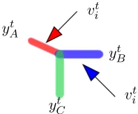
Figure 1: Schematic representation of the stochastic updates for the spectral estimation. Note the we never form the tensor explicitly, since the gradient involves vector products by collapsing two modes, as shown in Equation 17.

In Equation (17), all our tensor operations are in terms of efficient sample vector inner products, and no tensor is explicitly formed. The multilinear operations are shown in Figure 1. We chooseθ= 1 in our experiments to ensure that there is sufficient penalty for non-orthogonality, which prevents us from obtaining degenerate solutions.

After learning the decomposition of the third order moment, we perform post-processing to estimate Π.b

3.3 Post-processing

Eigenvalues Λ := [λ1, λ2, . . . , λk] are estimated as the norm of the eigenvectors λi =kφik3. Lemma 5 After we obtain Λ and Φ, the estimate for the topic-word matrix is given by

ˆ

µ=W>†Φ,

and in the community setting, the community membership matrix is given by

ˆ

ΠAc = diag(γ)1/3diag(Λ)−1Φ>Wˆ>GA,Ac.

where Ac := X∪B∪C. Similarly, we estimate ΠˆA by exchanging the roles of X and A. Next, we obtain the Dirichlet distribution parameters

ˆ

αi =γ2λ−_i 2,∀i∈[k].

whereγ2 is chosen such that we have normalizationP

i∈[k]αiˆ := P

i∈[k] αi α0 = 1.

Thus, we perform STGD method to estimate the eigenvectors and eigenvalues of the whitened tensor, and then use these to estimate the topic word matrix µ and community membership matrixΠ by thresholding.b

4. Implementation Details

4.1 Symmetrization Step to Compute M2

Note that for the topic model, the second order moment M2 can be computed easily from

the word-frequency vector. On the other hand, for the community setting, computing M2

and ZC in equation (7). This requires computation of pseudo-inverses of “Pairs” matrices.

Now, note that pseudo-inverse of (Pairs (B, C)) in Equation (7) can be computed using rank

k-SVD:

k-SVD (Pairs (B, C)) =UB(:,1 :k)ΣBC(1 :k)VC(:,1 :k)>.

We exploit the low rank property to have efficient running times and storage. We first implement the k-SVD of Pairs, given by G>_X,CGX,B. Then the order in which the matrix

products are carried out plays a significant role in terms of both memory and speed. Note thatZC involves the multiplication of a sequence of matrices of sizesRnA×nB,RnB×k,Rk×k, Rk×nC,G>x,CGx,Binvolves products of sizesRnC×k,Rk×k,Rk×nB, andZBinvolving products

of sizesRnA×nC,RnC×k,Rk×k,Rk×nB. While performing these products, we avoid products

of sizes RO(n)×O(n) and RO(n)×O(n). This allows us to have efficient storage requirements.

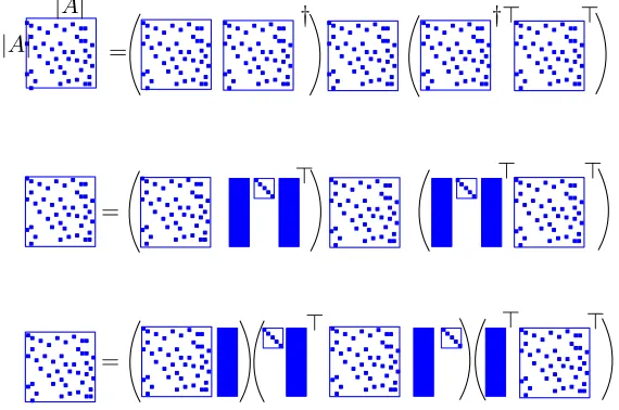
Such manipulations are represented in Figure 2.

=

† †> >

|A| |A|

=

> > >

=

> > >

Figure 2: By performing the matrix multiplications in an efficient order (Equation (10)), we avoid products involving O(n)×O(n) objects. Instead, we use objects of size O(n)×k which improves the speed, since k n. Equation (10) is

equiv-alent toM2 =

PairsA,BPairs†C,B

PairsC,B

Pairs†_B,C >

Pairs>_A,C −shift, where the shift = α0

α0+1 M1M1

>_{−diag M}

1M1>

. We do not explicitly calculate the pseudoinverse but maintain the low rank matrix decomposition form.

We then orthogonalize the third order moments to reduce the dimension of its modes to k. We perform linear transformations on the data corresponding to the partitions A,

B and C using the whitening matrix. The whitened data is thus yt A:=

D

W, G>_t,AE,yt B := D

W, ZBG>t,B E

, and yt C :=

D

W, ZCG>t,C E

4.2 Efficient Randomized SVD Computations

When we consider very large-scale data, the whitening matrix is a bottleneck to handle when we aim for fast running times. We obtain the low rank approximation of matrices using random projections. In the CPU implementation, we use tall-thin SVD (on a sparse matrix) via the Lanczos algorithm after the projection and in the GPU implementation, we use tall-thin QR. We give the overview of these methods below. Again, we use graph community membership model without loss of generality.

Randomized low rank approximation: From (Gittens and Mahoney, 2013), for the k -rank positive semi-definite matrix M2 ∈ RnA×nA with nA k, we can perform random

projection to reduce dimensionality. More precisely, if we have a random matrixS∈_RnA×_k˜

with unit norm (rotation matrix), we project M2 onto this random matrix to get Rn×k˜

tall-thin matrix. Note that we choose ˜k= 2k in our implementation. We will obtain lower dimension approximation of M2 in R˜kטk. Here we emphasize that S ∈ Rnטk is a random

matrix for dense M2. However for sparse M2, S ∈ {0,1}n× ˜

k _{is a column selection matrix}

with random sign for each entry.

After the projection, one approach we use is SVD on this tall-thin (Rn×k˜) matrix. Define

O :=M2S ∈Rnטk and Ω :=S>M2S∈R˜k×k˜. A low rank approximation of M2 is given by

OنO> (Gittens and Mahoney, 2013). Recall that the definition of a whitening matrixW

is that W>M2W =I. We can obtain the whitening matrix of M2 without directly doing a

SVD onM2 ∈RnA×nA.

Tall-thin SVD: This is used in the CPU implementation. The whitening matrix can be obtained by

W ≈(O†)>(Ω12)>. (18)

The pseudo code for computing the whitening matrix W using tall-thin SVD is given in Algorithm 2. Therefore, we only need to compute SVD of a tall-thin matrix O ∈_RnAט_k

.

Algorithm 2 Randomized Tall-thin SVD

Input: Second moment matrix M2. Output: Whitening matrixW.

1: Generate random matrixS ∈_Rnט_k

ifM2 is dense.

2: Generate column selection matrix with random signS ∈ {0,1}nטk _ifM

2 is sparse.

3: O=M2S∈_Rnט_k

4: [UO, LO, VO] =SVD(O)

5: Ω =S>O ∈_R˜kט_k

6: [UΩ, LΩ, VΩ] =SVD(Ω)

7: W =UOL−_O1V_O>VΩL

1 2

ΩU

>

Ω

Note that Ω∈R˜kטk, its square-root is easy to compute. Similarly, pseudoinverses can also

be obtained without directly doing SVD. For instance, the pseudoinverse of the Pairs (B, C) matrix is given by

(Pairs (B, C))†= (J†)>ΨJ†,

Algorithm 3 Randomized Pseudoinverse

Input: Pairs matrix Pairs (B, C).

Output: Pseudoinverse of the pairs matrix (Pairs (B, C))†. 1: Generate random matrixS ∈_Rn,k _ifM

2 is dense.

2: Generate column selection matrix with random signS ∈ {0,1}n×k ifM2 is sparse.

3: J = (Pairs (B, C))S

4: Ψ =S>J

5: [UJ, LJ, VJ] =SVD(J)

6: (Pairs (B, C))†=UJL−_J1V_J>ΨVJL−_J1U_J>

The sparse representation of the data allows for scalability on a single machine to datasets having millions of nodes. Although the GPU has SIMD architecture which makes parallelization efficient, it lacks advanced libraries with sparse SVD operations and out-of-GPU-core implementations. We therefore implement the sparse format on CPU for sparse datasets. We implement our algorithm using random projection for efficient dimensionality reduction (Clarkson and Woodruff, 2012) along with the sparse matrix operations available in the Eigen toolkit2, and we use the SVDLIBC (Berry et al., 2002) library to compute sparse SVD via the Lanczos algorithm. Theoretically, the Lanczos algorithm (Golub and Van Loan, 2013) on a n×n matrix takes around (2d+ 8)n flops for a single step whered

is the average number of non-zero entries per row.

Tall-thin QR: This is used in the GPU implementation due to the lack of library to do sparse tall-thin SVD. The difference is that we instead implement a tall-thin QR on O, therefore the whitening matrix is obtained as

W ≈Q(R†)>(Ω12)>.

The main bottleneck for our GPU implementation is device storage, since GPU memory is highly limited and not expandable. Random projections help in reducing the dimension-ality fromO(n×n) toO(n×k) and hence, this fits the data in the GPU memory better. Consequently, after the whitening step, we project the data intok-dimensional space. There-fore, the STGD step is dependent only on k, and hence can be fit in the GPU memory. So, the main bottleneck is computation of large SVDs. In order to support larger datasets such as the DBLP data set which exceed the GPU memory capacity, we extend our imple-mentation with out-of-GPU-core matrix operations and the Nystrom method (Gittens and Mahoney, 2013) for the whitening matrix computation and the pseudoinverse computation in the pre-processing module.

4.3 Stochastic updates

STGD can potentially be the most computationally intensive task if carried out naively since the storage and manipulation of a O(n3)-sized tensor makes the method not scalable. However we overcome this problem since we never form the tensor explicitly; instead, we collapse the tensor modes implicitly as shown in Figure 1. We gain large speed up by optimizing the implementation of STGD.To implement the tensor operations efficiently we

v_it yt

A,yBt,yCt

CPU

GPU

Standard Interface

v_it

y_At,y_Bt,y_Ct

CPU

GPU

Device Interface

v_it

Figure 3: Data transfers in the standard and device interfaces of the GPU implementation.

convert them into matrix and vector operations so that they are implemented using BLAS routines. We obtain whitened vectorsyA, yBandyC and manipulate these vectors efficiently to obtain tensor eigenvector updates using the gradient scaled by a suitable learning rate.

Efficient STGD via stacked vector operations: We convert the BLAS II into BLAS III operations by stacking the vectors to form matrices, leading to more efficient operations. Although the updating equation for the stochastic gradient update is presented serially in Equation (17), we can update thek eigenvectors simultaneously in parallel. The basic idea is to stack the k eigenvectorsφi ∈Rk into a matrix Φ, then using the internal parallelism

designed for BLAS III operations.

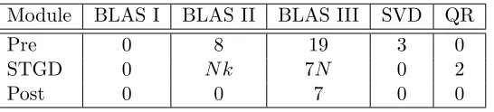
Overall, the STGD step involves 1 +k+i(2 + 3k) BLAS II overRkvectors, 7N BLAS III

overRk×k matrices and 2 QR operations over Rk×k matrices, where idenotes the number

of iterations. We provide a count of BLAS operations for various steps in Table 1.

Module BLAS I BLAS II BLAS III SVD QR

Pre 0 8 19 3 0

STGD 0 N k 7N 0 2

Post 0 0 7 0 0

Table 1: Linear algebraic operation counts: N denotes the number of iterations for STGD and k, the number of communities.

102 103 10−1

100 101 102 103 104

Number of communities

Time (in seconds) for 100 stochastic iterations

Scaling of the stochastic algorithm with the rank of the tensor

MATLAB Tensor Toolbox CULA Standard Interface CULA Device Interface Eigen Sparse

Figure 4: Comparison of the running time for STGD under differentkfor 100 iterations.

transfer (including whitened neighborhood vectors and the eigenvectors) at each stochastic iteration between the CPU memory and the GPU memory, the device interface involves allocating and retaining the eigenvectors at each stochastic iteration which in turn speeds up the spectral estimation.

We compare the running time of the CULA device code with the MATLAB code (using the tensor toolbox (Bader et al., 2012)), CULA standard code and Eigen sparse code in Figure 4. As expected, the GPU implementations of matrix operations are much faster and scale much better than the CPU implementations. Among the CPU codes, we notice that sparsity and optimization offered by the Eigen toolkit gives us huge gains. We obtain orders of magnitude of speed up for the GPU device code as we place the buffers in the GPU memory and transfer minimal amount of data involving the whitened vectors only once at the beginning of each iteration. The running time for the CULA standard code is more than the device code because of the CPU-GPU data transfer overhead. For the same reason, the sparse CPU implementation, by avoiding the data transfer overhead, performs better than the GPU standard code for very small number of communities. We note that there is no performance degradation due to the parallelization of the matrix operations. After whitening, the STGD requires the most code design and optimization effort, and so we convert that into BLAS-like routines.

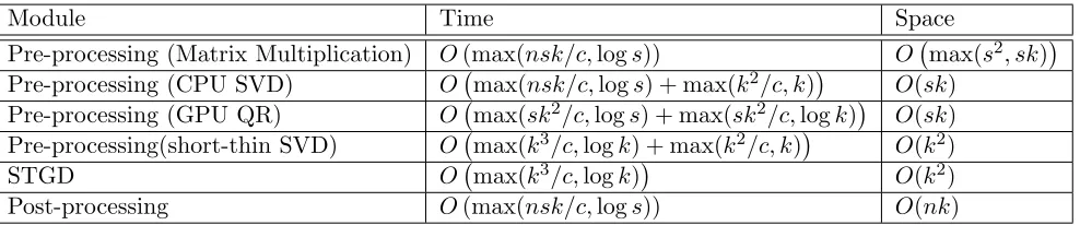
4.4 Computational Complexity

Module Time Space

Pre-processing (Matrix Multiplication) O(max(nsk/c,logs)) O max(s2, sk) Pre-processing (CPU SVD) O max(nsk/c,logs) + max(k2/c, k)

O(sk) Pre-processing (GPU QR) O max(sk2/c,logs) + max(sk2/c,logk)

O(sk) Pre-processing(short-thin SVD) O max(k3/c,logk) + max(k2/c, k) O(k2)

STGD O max(k3/c,logk) O(k2)

Post-processing O(max(nsk/c,logs)) O(nk)

Table 2: The time and space complexity (number of compute cores required) of our algo-rithm. Note that k n, s is the average degree of a node (or equivalently, the average number of non-zeros per row/column in the adjacency sub-matrix); note that the STGD time is per iteration time. We denote the number of cores as c -the time-space trade-off depends on this parameter.

The theoretical asymptotic complexity of our method is summarized in Table 2 and is best addressed by considering the parallel model of computation (J´aJ´a, 1992), i.e., wherein a number of processors or compute cores are operating on the data simultaneously in parallel. This is justified considering that we implement our method on GPUs and matrix products are embarrassingly parallel. Note that this is different from serial computational complexity. We now break down the entries in Table 2. First, we recall a basic lemma regarding the lower bound on the time complexity for parallel addition along with the required number of cores to achieve a speed-up.

Lemma 6 (J´aJ´a, 1992) Addition of snumbers in serial takes O(s) time; withΩ(s/logs)

cores, this can be improved to O(logs) time in the best case.

Essentially, this speed-up is achieved by recursively adding pairs of numbers in parallel.

Lemma 7 (J´aJ´a, 1992) ConsiderM ∈Rp×qandN ∈Rq×rwithsnon-zeros per row/column.

Naive serial matrix multiplication requires O(psr) time; with Ω(psr/logs) cores, this can be improved to O(logs) time in the best case.

Lemma 7 follows by simply parallelizing the sparse inner products and applying Lemma 6 for the addition in the inner products. Note that, this can be generalized to the fact that given ccores, the multiplication can be performed in O(max(psr/c,logs)) running time.

4.4.1 Pre-processing

Random projection: In preprocessing, givenccompute cores, we first do random projection using matrix multiplication. We multiply an O(n)×O(n) matrix M2 with an O(n)×O(k)

random matrix S. Therefore, this requiresO(nsk) serial operations, wheresis the number of non-zero elements per row/column ofM2. Using Lemma 7, givenc= _lognsk_s cores, we could achieveO(logs) computational complexity. However, the parallel computational complexity is not further reduced with more than _lognsk_s cores.

Tall-thin SVD: We perform Lanczos SVD on the tall-thin sparse O(n)×O(k) matrix, which involves a tri-diagonalization followed with the QR on the tri-diagonal matrix. Given

c= _lognsk_s cores, the computational complexity of the tri-diagonalization isO(logs). We then do QR on the tridiagonal matrix which is as cheap asO(k2) serially. Each orthogonalization requiresO(k) inner products of constant entry vectors, and there areO(k) such orthogonal-izations to be done. Therefore given O(k) cores, the complexity isO(k). More cores does not help since the degree of parallelism is k.

Tall-thin QR: Alternatively, we perform QR in the GPU implementation which takes

O(sk2). To arrive at the complexity of obtaining Q, we analyze the Gram-Schmidt or-thonormalization procedure under sparsity and parallelism conditions. Consider a serial Gram-Schmidt on k columns (which are s-dense) of O(n)×O(k) matrix. For each of the columns 2 to k, we perform projection on the previously computed components and sub-tract it. Both inner product and subsub-traction operations are on the s-dense columns and there are O(s) operations which are doneO(k2) times serially. The last step is the normal-ization of k s-dense vectors with is an O(sk) operation. This leads to a serial complexity of O(sk2+sk) = O(sk2). Using this, we may obtain the parallel complexity in different regimes of the number of cores as follows.

Parallelism for inner products : For each componenti, we needi−1 projections on pre-vious components which can be parallel. Each projection involves scaling and inner product operations on a pair of s-dense vectors. Using Lemma 6, projection for component i can be performed inO(max(sk_c,logs)) time. O(logs) complexity is obtained usingO(sk/logs) cores.

Parallelism for subtractions: For each component i, we need i−1 subtractions on a

s-dense vector after the projection. Serially the subtraction requiresO(sk) operations, and this can be reduced toO(logk) withO(sk/logk) cores in the best case. The complexity is

O(max(sk_c,logk)).

Combing the inner products and subtractions, the complexity is O max(sk_c,logs) + max(sk_c,logk)

for componenti. There arekcomponents in total, which can not be

par-allel. In total, the complexity for the parallel QR is Omax(sk_c2,logs) + max(sk_c2,logk).

Short-thin SVD: SVD of the smallerO(Rk×k) matrix time requiresO(k3) computations

in serially. We note that this is the bottleneck for the computational complexity, but we emphasize thatkis sufficiently small in many applications. Furthermore, thisk3_complexity

can be reduced by using distributed SVD algorithms e.g. (Kannan et al., 2014; Feldman et al., 2013). An analysis with respect to Lanczos parallel SVD is similar with the discussion in the Tall-thin SVD paragraph. The complexity is O(max(k3_{/c,logk) + max(k}2_{/c, k)). In}

the best case, the complexity is reduced toO(logk+k).

The serial time complexity of SVD is O(n2_{k) but with randomized dimensionality}

re-duction (Gittens and Mahoney, 2013) and parallelization (Constantine and Gleich, 2011), this is significantly reduced.

4.4.2 STGD

inner products in parallel withccompute cores since each core can perform an inner product to compute an element in the resulting matrix independent of other cores in linear time. Forc∈(k3/logk,∞], using Lemma 6, we obtain a running time ofO(logk). Note that the STGD time complexity is calculated per iteration.

4.4.3 Post-processing

Finally, post-processing consists of sparse matrix products as well. Similar to pre-processing, this consists of multiplications involving the sparse matrices. Givensnumber of non-zeros per column of an O(n)×O(k) matrix, the effective number of elements reduces to O(sk). Hence, givenc∈[1, nks/logs] cores, we needO(nsk/c) time to perform the inner products for each entry of the resultant matrix. Forc∈(nks/logs,∞], using Lemma 6, we obtain a running time of O(logs).

Note thatnk2 is the complexity of computing the exact SVD and we reduce it toO(k) when there are sufficient cores available. This is meant for the setting wherekis small. This

k3 complexity of SVD on O(k×k) matrix can be reduced to O(k) using distributed SVD algorithms e.g. (Kannan et al., 2014; Feldman et al., 2013). We note that the variational inference algorithm complexity, by Gopalan and Blei (Gopalan and Blei, 2013), is O(mk) for each iteration, where m denotes the number of edges in the graph, and n < m < n2. In the regime thatn k, our algorithm is more efficient. Moreover, a big difference is in the scaling with respect to the size of the network and ease of parallelization of our method compared to variational one.

5. Validation methods

5.1 p-value testing:

$\Pi_{1}$

$\Pi_{2}$

$\Pi_{3}$

$\Pi_{4}$

$\hat{\Pi}_{1}$

$\hat{\Pi}_{2}$

$\hat{\Pi}_{3}$

$\hat{\Pi}_{4}$

$\hat{\Pi}_{5}$

$\hat{\Pi}_{6}$

Figure 5: Bipartite graph G{Pval} induced by p-value testing. Edges represent statistically

significant relationships between ground truth and estimated communities.

b

Π be denoted by Πb_i. Our community detection method is unsupervised, which inevitably results in row permutations between Π andΠ andb bkmay not be the same ask. To validate the results, we need to find a good match between the rows ofΠ and Π. We use the notionb ofp-values to test for statistically significant dependencies among a set of random variables. The p-value denotes the probability of not rejecting the null hypothesis that the random variables under consideration are independent and we use the Student’s3 t-test statistic (Fa-dem, 2012) to compute thep-value. We use multiple hypothesis testing for different pairs of estimated and ground-truth communities Πbi,Π_j and adjust the p-values to ensure a small enough false discovery rate (FDR) (Strimmer, 2008).

The test statistic used for the p-value testing of the estimated communities is

Tij :=

ρ

b Πi,Πj

√ n−2

r

1−ρΠb_i,Π_j 2

.

The rightp-value is obtained via the probability of obtaining a value (saytij) greater than

the test statisticTij, and it is defined as

Pval(Πi,Πb_j) := 1−_P(tij > Tij).

Note that Tij has Student’s t-distribution with degree of freedom n−2 (i.e. Tij ∼tn−2).

Thus, we obtain the right p-value4_.

In this way, we compute the Pval matrix as

Pval(i, j) :=Pval h

b Πi,Πj

i

,∀i∈[k] and j∈[bk].

5.2 Evaluation metrics

Recovery ratio: Validating the results requires a matching of the true membership Π with estimated membershipΠ. Letb P_val(Π_i,Πb_j) denote the rightp-value under the null hypothesis that ΠiandΠb_j are statistically independent. We use thep-value test to find out pairs Πi,Πb_j which pass a specified p-value threshold, and we denote such pairs using a bipartite graph

G{Pval}. Thus, G{Pval} is defined as

G{Pval} :=

n V_{(1)_P

val}, V

(2)

{Pval}

o

, E{Pval}

,

where the nodes in the two node sets are

V_{(1)_P

val} ={Π1, . . . ,Πk},

V_{(2)_P

val} =

n b

Π1, . . . ,Πb b k o

3. Note that Student’st-test is robust to the presence of unequal variances when the sample sizes of the two are equal which is true in our setting.

and the edges ofG{Pval} satisfy

(i, j)∈E{Pval} s.t. Pval

h b Πi,Πj

i

≤0.01.

A simple example is shown in Figure 5, in which Π2 has statistically significant

depen-dence withΠb1, i.e., the probability of not rejecting the null hypothesis is small (recall that

null hypothesis is that they are independent). If no estimated membership vector has a significant overlap with Π3, then Π3 is not recovered. There can also be multiple pairings

such as for Π1 and {Πb₂,Πb3,Πb₆}. The p-value test between Π₁ and {Πb2,Πb3,Πb₆} indicates that probability of not rejecting the null hypothesis is small, i.e., they are independent. We use 0.01 as the threshold. The same holds for Π2 and{Πb₁}and for Π₄ and{Πb4,Πb₅}. There can be a perfect one to one matching like for Π2and Πb₁ as well as a multiple matching such as for Π1 and {Πb₂,Πb₃,Πb₆}. Or another multiple matching such as for{Π₁,Π₂} andΠb₃.

Let Degree_i denote the degree of ground truth community i∈[k] in G{Pval}, we define

the recovery ratio as follows.

Definition 8 The recovery ratio is defined as

R:= 1

k X

i

I{Degreei >0}, i∈[k]

where I(x) is the indicator function whose value equals one if x is true.

The perfect case is that all the memberships have at least one significant overlapping es-timated membership, giving a recovery ratio of 100%. Error function: For performance analysis of our learning algorithm, we use an error function given as follows:

Definition 9 The average error function is defined as

E := 1

k

X

(i,j)∈E{P_val}

 

 1

n X

x∈|X|

b

Πi(x)−Πj(x)

 

 ,

where E{Pval} denotes the set of edges based on thresholding of the p-values.

The error function incorporates two aspects, namely the l1 norm error between each estimated community and the corresponding paired ground truth community, and the error induced by false pairings between the estimated and ground-truth communities through

p-value testing. For the former l1 norm error, we normalize with n which is reasonable and results in the range of the error in [0,1]. For the latter, we define the average error function as the summation of all paired memberships errors divided by the true number of communities k. In this way we penalize falsely discovered pairings by summing them up. Our error function can be greater than 1 if there are too many falsely discovered pairings through p-value testing (which can be as large ask×bk).

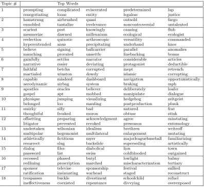
Hardware / software Version

CPU Dual 8-core Xeon @ 2.0GHz

Memory 64GB DDR3

GPU Nvidia Quadro K5000

CUDA Cores 1536

Global memory 4GB GDDR5

CentOS Release 6.4 (Final)

GCC 4.4.7

CUDA Release 5.0

CULA-Dense R16a

Table 3: System specifications.

people and bridgeness analyzes the extent to which a given vertex is shared among different communities (Nepusz et al., 2008). Formally, the bridgeness of a vertexiis defined as

bi := 1− v u u u t

b k

b k−1

b k X

j=1

b Πi(j)−

1

b k

2

. (19)

Note that centrality measures should be used in conjunction with bridge score to distinguish outliers from genuine bridge nodes (Nepusz et al., 2008). The degree-corrected bridgeness

is used to evaluate our results and is defined as

B_i :=Dibi, (20)

whereDi is degree of node i.

6. Experimental Results

The specifications of the machine on which we run our code are given in Table 3.

Results on Synthetic Datasets:

We perform experiments for both the stochastic block model (α0 = 0) and the mixed

membership model. For the mixed membership model, we set the concentration parameter

α0 = 1. We note that the error is around 8%−14% and the running times are under a

minute, whenn≤10000 andnk5_.

We observe that more samples result in a more accurate recovery of memberships which matches intuition and theory. Overall, our learning algorithm performs better in the stochastic block model case than in the mixed membership model case although we note that the accuracy is quite high for practical purposes. Theoretically, this is expected since smaller concentration parameter α0 is easier for our algorithm to learn (Anandku-mar et al., 2013b). Also, our algorithm is scalable to an order of magnitude more in nas illustrated by experiments on real-world large-scale datasets.

5. The code is available at

Note that we threshold the estimated memberships to clean the results. There is a tradeoff between match ratio and average error via different thresholds. In synthetic exper-iments, the tradeoff is not evident since a perfect matching is always present. However, we need to carefully handle this in experiments involving real data.

Results on Topic Modeling:

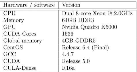
We perform experiments for the bag of words data set (Bache and Lichman, 2013) for The New York Times. We set the concentration parameter to be α0 = 1 and observe top recovered words in numerous topics. The results are in Table 4. Many of the results are expected. For example, the top words in topic # 11 are all related to some bad personality. We also present the words with most spread membership, i.e., words that belong to many topics as in Table 5. As expected, we see minutes, consumer, human, member and so on. These words can appear in a lot of topics, and we expect them to connect topics.

Topic # Top Words

1 prompting complicated eviscerated predetermined lap renegotiating loose entity legalese justice

2 hamstrung airbrushed quasi outsold fargo

ennobled tantalize irrelevance noncontroversial untalented

3 scariest pest knowingly causing flub

mesmerize dawned millennium ecological ecologist 4 reelection quixotic arthroscopic versatility commanded

hyperextended anus precipitating underhand knee 5 believe signing ballcarrier parallel anomalies

munching prorated unsettle linebacking bonus 6 gainfully settles narrator considerable articles

narrative rosier deviating protagonist deductible

7 faithful betcha corrupted inept retrench

martialed winston dowdy islamic corrupting 8 capable misdeed dashboard navigation opportunistically

aerodynamic airbag system braking mph

9 apostles oracles believer deliberately loafer

gospel apt mobbed manipulate dialogue

10 physique jumping visualizing hedgehog zeitgeist belonged loo mauling postproduction plunk

11 smirky silly bad natured frat

thoughtful freaked moron obtuse stink

12 offsetting preparing acknowledgment agree misstating litigator prevented revoked preseason entomology 13 undertaken wilsonian idealism brethren writeoff

multipolar hegemonist multilateral enlargement mutating 14 athletically fictitious myer majorleaguebaseball familiarizing

resurrect slug backslide superseding artistically

15 dialog files diabolical lion town

password list swiss coldblooded outgained

16 recessed phased butyl lowlight balmy

redlining prescription marched mischaracterization tertiary 17 sponsor televise sponsorship festival sullied

ratification insinuating warhead staged reconstruct 18 trespasses buckle divestment schoolchild refuel

ineffectiveness coexisted repentance divvying overexposed

Keywords

minutes, consumer, human, member, friend, program, board, cell, insurance, shot

Table 5: The top ten words which occur in multiple contexts in the New York Times dataset.

Results on Real-world Graph Datasets: We describe the results on real datasets sum-marized in Table 6 in detail below. The simulations are sumsum-marized in Table 7.

Statistics Facebook Yelp DBLP sub DBLP

|E| 766,800 672,515 5,066,510 16,221,000

|V| 18,163 10,010+28,588 116,317 1,054,066

GD 0.004649 0.000903 0.000749 0.000029

k 360 159 250 6,003

AB 0.5379 0.4281 0.3779 0.2066

ADCB 47.01 30.75 48.41 6.36

Table 6: Summary of real datasets used in our paper: |V| is the number of nodes in the graph, |E| is the number of edges, GD is the graph density given by _|V|(2_||_VE_|−| ₁₎,

k is the number of communities, AB is the average bridgeness and ADCB is the average degree-corrected bridgeness(explained in Section 5).

The results are presented in Table 7. We note that our method, in both dense and sparse implementations, performs very well compared to the state-of-the-art variational method. For the Yelp dataset, we have a bipartite graph where the business nodes are on one side and user nodes on the other and use the review stars as the edge weights. In this bipartite setting, the variational code provided by Gopalan et al (Gopalan et al., 2012) does not work on since it is not applicable to non-homophilic models. Our approach does not have this restriction. Note that we use our dense implementation on the GPU to run experiments with large number of communities k as the device implementation is much faster in terms of running time of the STGD step.On the other hand, the sparse implementation on CPU is fast and memory efficient in the case of sparse graphs with a small number of communities while the dense implementation on GPU is faster for denser graphs such as Facebook. Note that data reading time for DBLP is around 4700 seconds, which is not negligible as compared to other datasets (usually within a few seconds). Effectively, our algorithm, excluding the file I/O time, executes within two minutes for k= 10 and within ten minutes for k= 100.

Interpretation on Yelp Dataset: The ground truth on business attributes such as location and type of business are available (but not provided to our algorithm) and we provide the distribution in Figure 6 on the left side. There is also a natural trade-off between recovery ratio and average error or between attempting to recover all the business communities and the accuracy of recovery. We can either recover top significant communities with high accuracy or recover more with lower accuracy. We demonstrate the trade-off in Figure 6 on the right side.

Data Method bk Thre E R(%) Time(s) Ten(sparse) 10 0.10 0.063 13 35 Ten(sparse) 100 0.08 0.024 62 309 Ten(sparse) 100 0.05 0.118 95 309 Ten(dense) 100 0.100 0.012 39 190 Ten(dense) 100 0.070 0.019 100 190 FB Variational 100 – 0.070 100 10,795

Ten(dense) 500 0.020 0.014 71 468 Ten(dense) 500 0.015 0.018 100 468 Variational 500 – 0.031 100 86,808 Ten(sparse) 10 0.10 0.271 43 10 Ten(sparse) 100 0.08 0.046 86 287 Ten(dense) 100 0.100 0.023 43 1,127 YP Ten(dense) 100 0.090 0.061 80 1,127 Ten(dense) 500 0.020 0.064 72 1,706 Ten(dense) 500 0.015 0.336 100 1,706 Ten(dense) 100 0.15 0.072 36 7,664 Ten(dense) 100 0.09 0.260 80 7,664 Variational 100 – 7.453 99 69,156 DB sub Ten(dense) 500 0.10 0.010 19 10,157 Ten(dense) 500 0.04 0.139 89 10,157 Variational 500 – 16.38 99 558,723 Ten(sparse) 10 0.30 0.103 73 4716 DB Ten(sparse) 100 0.08 0.003 57 5407 Ten(sparse) 100 0.05 0.105 95 5407

Table 7: Yelp, Facebook and DBLP main quantitative evaluation of the tensor method ver-sus the variational method: bkis the community number specified to our algorithm, Thre is the threshold for picking significant estimated membership entries. Refer to Table 6 for statistics of the datasets.

Business RC Categories

Four Peaks Brewing Co 735 Restaurants, Bars, American (New), Nightlife, Food, Pubs, Tempe

Pizzeria Bianco 803 Restaurants, Pizza,Phoenix

FEZ 652 Restaurants, Bars, American (New), Nightlife, Mediterranean, Lounges Phoenix

Matt’s Big Breakfast 689 Restaurants, Phoenix, Breakfast& Brunch

Cornish Pasty Company 580 Restaurants, Bars, Nightlife, Pubs, Tempe

Postino Arcadia 575 Restaurants, Italian, Wine Bars, Bars, Nightlife, Phoenix

Cibo 594 Restaurants, Italian, Pizza, Sandwiches, Phoenix

Phoenix Airport 862 Hotels & Travel, Phoenix

Gallo Blanco Cafe 549 Restaurants, Mexican, Phoenix

The Parlor 489 Restaurants, Italian, Pizza, Phoenix

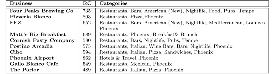
Table 8: Top 10 bridging businesses in Yelp and categories they belong to. “RC” denotes review counts for that particular business.

0 50 100 150 200 250 300 0

50 100 150 200 250 300

Distribution of Categories:

Number of categories

Number of business

0 0.2 0.4 0.6 0.8 1

0 0.05 0.1 0.15 0.2 0.25 0.3 0.35

match ratio

average error

Figure 6: Distribution of business categories (left) and result tradeoff between recovery ratio and error for yelp (right).

the “niche” categories with a dedicated set of reviewers, who mostly do not review other categories.

Category Business Star(B) Star(C) RC(B) RC(C) Latin American Salvadoreno 4.0 3.94 36 93.8 Gluten Free P.F. Chang’s 3.5 3.72 55 50.6 Hobby Shops Make Meaning 4.5 4.13 14 7.6 Mass Media KJZZ 91.5FM 4.0 3.63 13 5.6

Yoga Sutra Midtown 4.5 4.55 31 12.6

Churches St Andrew Church 4.5 4.52 3 4.2 Art Galleries Sette Lisa 4.5 4.48 4 6.6 Libraries Cholla Branch 4.0 4.00 5 11.2 Religious St Andrew Church 4.5 4.40 3 4.2 Wickenburg Taste of Caribbean 4.0 3.66 60 6.7

Table 9: Most accurately recovered categories and businesses with highest membership weights for the Yelp dataset. “Star(B)” denotes the review stars that the business receive and “Star(C)”, the average review stars that businesses in that category receive. “RC(B)” denotes the review counts for that business and “RC(C)” , the average review counts in that category.

where kc := 134 is the number of remaining categories and n := 10141 is the number of

business remaining after removing all the negligible categories. All the businesses collected in the Yelp data are in AZ except 3 of them (one is in CA, one in CO and the other in SC). We remove the three businesses outside AZ. We notice that most of the businesses are spread out in 25 cities. Community membership matrix for location is defined as Π∈Rkl×n

where kl := 25 is the number cities and n := 10010 is number of businesses. Distribution

of locations are in Table 11. The stars a business receives can vary from 1 (the lowest) to 5 (the highest). The higher the score is, the more satisfied the customers are. The average star score is 3.6745. The distribution is given in Table 10. There are also review counts for each business which are the number of reviews that business receives from all the users. The minimum review counts is 3 and the maximum is 862. The mean of review counts is 20.1929. The preprocessing helps us to pick out top communities.

There are 5 attributes associated with all the 11537 businesses, which are “open”, “Cat-egories”, “Location”, “Review Counts” and “Stars”. We model ground truth communities as a combination of “Categories” and “Location”. We select business categories with more than 20 members and remove all businesses which are closed. 10010 businesses are re-mained. Only 28588 users are involved in reviews towards the 10010 businesses. There are 3 attributes associated with all the 28588 users, which are “Female”, “Male”, “Review Counts” and “Stars”. Although we do not directly know the gender information from the dataset, a name-gender guesser6 _{is used to estimate gender information using names.}

Star Score Num of businesses Percentage

1.0 108 0.94%

1.5 170 1.47%

2.0 403 3.49%

2.5 1011 8,76%

3.0 1511 13.10%

3.5 2639 22.87%

4.0 2674 23.18%

4.5 1748 15.15%

5.0 1273 11.03%

Table 10: Table for distribution of business star scores.

We provide some sample visualization results in Figure 7 for both the ground truth and the estimates from our algorithm. We sub-sample the users and businesses, group the users into male and female categories, and consider nail salon and tire businesses. Analysis of ground truth reveals that nail salon and tire businesses are very discriminative of the user genders, and thus we employ them for visualization. We note that both the nail salon and tire businesses are categorized with high accuracy, while users are categorized with poorer accuracy.

Our algorithm can also recover the attributes of users. However, the ground truth available about users is far more limited than businesses, and we only have information on gender, average review counts and average stars (we infer the gender of the users through

City State Num of business

Anthem AZ 34

Apache Junction AZ 46

Avondale AZ 129

Buckeye AZ 31

Casa Grande AZ 48

Cave Creek AZ 65

Chandler AZ 865

El Mirage AZ 11

Fountain Hills AZ 49

Gilbert AZ 439

Glendale AZ 611

Goodyear AZ 126

Laveen AZ 22

Maricopa AZ 31

Mesa AZ 898

Paradise Valley AZ 57

Peoria AZ 267

Phoenix AZ 4155

Queen Creek AZ 78

Scottsdale AZ 2026

Sun City AZ 37

Surprise AZ 161

Tempe AZ 1153

Tolleson AZ 22

Wickenburg AZ 28

Table 11: Distribution of business locations. Only top cities with more than 10 businesses are presented.

Tires

Male Female

Nail Salon Tires

Male Female

Nail Salon

Figure 7: Ground truth (left) vs estimated business and user categories (right). The error in the estimated graph due to misclassification is shown by the mixed colours.

the characteristics of their users, for delivering better personalized advertisements for users, and so on.

Facebook Dataset: A snapshot of the Facebook network of UNC (Traud et al., 2010) is provided with user attributes. The ground truth communities are based on user attributes given in the dataset which are not exposed to the algorithm. There are 360 top communities with sufficient (at least 20) users. Our algorithm can recover these attributes with high accuracy; see main paper for our method’s results compared with variational inference result (Gopalan et al., 2012).

We also obtain results for a range of values ofα0(Figure 8). We observe that the recovery ratio improves with largerα0 since a largerα0 can recover overlapping communities more

efficiently while the error score remains relatively the same.

0 0.05 0.1 0.15 0.2

0 0.2 0.4 0.6 0.8 1

Threshold

Recovery ratio

alpha0.1 alpha0.5 alpha0.9

0 0.05 0.1 0.15 0.2

0 0.05 0.1 0.15 0.2 0.25

Threshold

Error

alpha0.1 alpha0.5 alpha0.9

Figure 8: Performance analysis of Facebook dataset under different settings of the concen-tration parameter (α0) for ˆk= 100.

For the Facebook dataset, the top ten communities recovered with lowest error consist of certain high schools, second majors and dorms/houses. We observe that high school attributes are easiest to recover and second major and dorm/house are reasonably easy to recover by looking at the friendship relations in Facebook. This is reasonable: college students from the same high school have a high probability of being friends; so do colleges students from the same dorm.

DBLP Dataset:

The DBLP data contains bibliographic records7 with various publication venues, such as journals and conferences, which we model as communities. We then consider authors who have published at least one paper in a community (publication venue) as a member of it. Co-authorship is thus modeled as link in the graph in which authors are represented as nodes. In this framework, we could recover the top authors in communities and bridging authors.

7. Conclusion

In this paper, we presented a fast and unified moment-based framework for learning over-lapping communities as well as topics in a corpus. There are several key insights involved. Firstly, our approach follows from a systematic and guaranteed learning procedure in con-trast to several heuristic approaches which may not have strong statistical recovery guaran-tees. Secondly, though using a moment-based formulation may seem computationally expen-sive at first sight, implementing implicit “tensor” operations leads to significant speed-ups of the algorithm. Thirdly, employing randomized methods for spectral methods is promising in the computational domain, since the running time can then be significantly reduced.

This paper paves the way for several interesting directions for further research. While our current deployment incorporates community detection in a single graph, extensions to multi-graphs and hypermulti-graphs are possible in principle. A careful and efficient implementation for such settings will be useful in a number of applications. It is natural to extend the deployment to even larger datasets by having cloud-based systems. The issue of efficient partitioning of data and reducing communication between the machines becomes significant there. Combining our approach with other simple community detection approaches to gain even more speedups can be explored.

Acknowledgement

The first author is supported by NSF BIGDATA IIS-1251267, the second author is supported in part by UCI graduate fellowship and NSF Award CCF-1219234, and the last author is supported in part by Microsoft Faculty Fellowship, NSF Career award CCF-1254106, NSF Award CCF-1219234, and ARO YIP Award W911NF-13-1-0084. The authors acknowledge insightful discussions with Prem Gopalan, David Mimno, David Blei, Qirong Ho, Eric Xing, Carter Butts, Blake Foster, Rui Wang, Sridhar Mahadevan, and the CULA team. Special thanks to Prem Gopalan and David Mimno for providing the variational code and answer-ing all our questions. The authors also thank Daniel Hsu and Sham Kakade for initial discussions regarding the implementation of the tensor method. We also thank Dan Melzer for helping us with the system-related issues.

Appendix A. Stochastic Updates

After obtaining the whitening matrix, we whiten the data G>_x,A, G>_x,B and G>_x,C by linear operations to get y_At,y_Bt andy_Ct ∈_Rk_:

yt_A:=DG>_x,A, WE, yt_B:=DZBG>x,B, W E

, y_Ct :=DZCG>x,C, W E

.

The stochastic gradient descent algorithm is obtained by taking the derivative of the loss function ∂L_∂vit(v):

∂Lt(v)

∂vi

=θ k X

j=1

hvj, vii2vj−

(α0+ 1)(α0+ 2) 2

vi, yAt vi, ytB

y_Ct −α2₀φt_i,y¯A φti,y¯Bt

¯

yC

+α0(α0+ 1) 2

φt_i, y_At φ_it, y_Bty¯C +

α0(α0+ 1) 2

φt_i, y_At φt_i,y¯B

yC

+α0(α0+ 1) 2

φt_i,y¯A φti, yBt

yC

for i ∈ [k], where yt_A, y_Bt and yt_C are the online whitened data points as discussed in the whitening step and θ is a constant factor that we can set.

The iterative updating equation for the stochastic gradient update is given by

φt+1_i ←φt_i−βt∂L t ∂vi φt i (21)

for i∈ [k], where βt is the learning rate, φt_i is the last iteration eigenvector and φt_i is the updated eigenvector. We update eigenvectors through

φt+1_i ←φt_i−θβt k X

j=1 h

φt_j, φt_i2φt_j i

+ shift[βtφt_i, yt_A φt_i, y_Btyt_C] (22)

Now we shift the updating steps so that they correspond to the centered Dirichlet moment forms, i.e.,

shift[βt

φt_i, y_At φt_i, y_Bt

y_Ct] :=βt(α0+ 1)(α0+ 2)

2

φt_i, yt_A φt_i, yt_B y_Ct

+βtα2₀φt_i,yA¯ φt_i,yB¯ yC¯ −βtα0(α0+ 1)

2

φt_i, yt_A φt_i, y_BtyC¯

−βtα0(α0+ 1)

2

φt_i, yt_A φt_i,y¯B

yC−βt

α0(α0+ 1)

2

φt_i,y¯A φti, yBt

yC, (23)

where ¯yA:=Et[ytA] and similarly for ¯yB and ¯yC.

Appendix B. Proof of correctness of our algorithm:

We now prove the correctness of our algorithm. First, we compute M2 as just

Ex h

˜

G>_x,C⊗G˜>_x,B|ΠA,ΠB,ΠC i

where we define

˜

G>_x,B :=Ex

G>_x,A⊗G>_x,C

ΠA,ΠC Ex

G>_x,B⊗G>_x,C

ΠB,ΠC †

G>_x,B

˜

G>_x,C :=Ex

G>_x,A⊗G>_x,B

ΠA,ΠB Ex

G>_x,C⊗G>_x,B

ΠB,ΠC †