Provably Efficient Learning with Typed Parametric Models

Provably Efficient Learning with Typed Parametric Models

Emma Brunskill [email protected]

Computer Science and Artificial Intelligence Laboratory Massachusetts Institute of Technology

Cambridge, MA 02143, USA

Bethany R. Leffler [email protected]

Lihong Li [email protected]

Michael L. Littman [email protected]

Department of Computer Science Rutgers University

Piscataway, NJ 08854, USA

Nicholas Roy [email protected]

Computer Science and Artificial Intelligence Laboratory Massachusetts Institute of Technology

Cambridge, MA 02143, USA

Editor: Sham Kakade

Abstract

To quickly achieve good performance, reinforcement-learning algorithms for acting in large continuous-valued domains must use a representation that is both sufficiently powerful to capture important domain characteristics, and yet simultaneously allows generalization, or sharing, among experiences. Our algorithm balances this tradeoff by using a stochastic, switching, parametric dy-namics representation. We argue that this model characterizes a number of significant, real-world domains, such as robot navigation across varying terrain. We prove that this representational as-sumption allows our algorithm to be probably approximately correct with a sample complexity that scales polynomially with all problem-specific quantities including the state-space dimension. We also explicitly incorporate the error introduced by approximate planning in our sample complexity bounds, in contrast to prior Probably Approximately Correct (PAC) Markov Decision Processes (MDP) approaches, which typically assume the estimated MDP can be solved exactly. Our experi-mental results on constructing plans for driving to work using real car trajectory data, as well as a small robot experiment on navigating varying terrain, demonstrate that our dynamics representation enables us to capture real-world dynamics in a sufficient manner to produce good performance.

Keywords: reinforcement learning, provably efficient learning

1. Introduction

learning the best route to drive to work, or how a remote robotic rover can learn to traverse different types of terrain. To perform learning efficiently in such environments, we will assume that the world dynamics can be compactly described by a small set of simple parametric models, such as one for driving on highways and another for driving on small roads. We will prove that this assumption allows our algorithm to require an amount of experience that only scales polynomially with the state space dimension. We will also empirically demonstrate that these assumptions are realistic for several real world data sets, indicating that our Continuous-Offset Reinforcement Learning (CORL) algorithm may be well suited for large, high-dimensional domains.

A critical choice in the construction of a reinforcement-learning algorithm is how to balance between actions that gather information about the world environment (exploration) versus actions that are expected to yield high reward given the agent’s current estimates of the world environment (exploitation). In early work, algorithms such as Q-learning were shown to perform optimally in the limit of infinite data (Watkins, 1989), but no finite-sample guarantees were known. More recently there have been three main branches of model-based reinforcement learning research concerned with the exploration problem. The first consists of heuristic approaches, some of which perform very well in practice, but lack performance guarantees (for example Jong and Stone 2007). The second branch strives to perform the action that optimally balances exploration and exploitation at each step. Such Bayesian approaches include the model parameters inside the state space of the problem. Poupart et al. (2006) assumed a fully observed discrete state space and modeled the un-derlying model parameters as hidden states, effectively turning the problem into a continuous-state partially observable Markov decision process (POMDP). Castro and Precup (2007) also assumed a fully observed discrete state space but represented the model parameters as counts over the dif-ferent transitions and reward received, thereby keeping the problem fully observable. Doshi et al. (2008) considered a Bayesian approach for learning when the discrete state space is only partially observable, and Ross et al. (2008) considered learning in a partially-observed continuous-valued robot navigation problem. Approaches in the Bayesian RL framework run into inherent complex-ity problems and typically produce algorithms that only approximately solve their target optimalcomplex-ity criteria.

Within the PAC-MDP line of research, there has been little work on directly considering continuous-valued states. One exception is the work of Strehl and Littman (2008), who consid-ered learning in continuous-valued state-action spaces. Their work assumed that a single dynamics representation was shared among all states, and that the noise parameter of the dynamics represen-tation was known. The focus of their paper was slightly different than the current work, in that the authors presented a new online regression algorithm for determining when enough information was known to make accurate predictions.

An alternate approach to handling continuous state spaces is to discretize the space into a grid. This step enables prior PAC-MDP algorithms such as R-max (Brafman and Tennenholtz, 2002) to be applied directly to the discretized space. However, their representation of the world may not fully exploit existing structure. In particular, such a representation requires that the dynamics model for each state-action tuple is learned independently. Since each state-action can have entirely different dynamics, this approach has a great deal of representational power. However, as there is no sharing of dynamics information among states, it has a very low level of generalization. In contrast, the work of Strehl and Littman (2008) and the classic linear quadratic Gaussian regulator model (Burl, 1998) assume that the dynamics model is the same for all states, greatly restricting the representational power of these models in return for higher generalization and fast learning.

Recently, there have been several approaches that explore the middle ground of representational power and generalization ability. Jong and Stone (2007) assumed that the dynamics model between nearby states was likely to be similar, and used an instance-based approach to solve a continuous-state RL problem. Their experimental results were encouraging but no theoretical guarantees were provided, and the amount of data needed would typically scale exponentially with the state-space dimension. A stronger structural assumption is made in the work of Leffler et al. (2007), which focused on domains in which the discrete state space is divided into a set of types. States within the same type were assumed to have the same dynamics. The authors proved that a typed representation can require significantly less experience to achieve good performance compared to a standard R-max algorithm that learns each state-action dynamics model separately.

Our work draws on the recent progress and focuses on continuous-state, discrete-action, typed problems. By using a parametric model to represent the dynamics of each of a discrete set of types, we sacrifice some of the representational power of prior approaches (Leffler et al., 2007; Brafman and Tennenholtz, 2002) in return for improved generalization, but still retain a much more flexible representation than approaches that assume a single dynamics model that is shared across all states. In particular, we prove that restricting our representational power enables our algorithm to have a sample complexity that scales polynomially with the state-space dimension. An alternate approach is to place a uniformly spaced grid over the state space and solve the problem using the existing algorithms from Leffler et al. (2007) or Brafman and Tennenholtz (2002). However, this strategy results in an algorithm whose computational complexity scales exponentially with the state-space dimension.

In particular, our dynamics representation is a simple noisy offset model, where the next state is presumed to be a function of the prior state, plus an offset and some Gaussian distributed noise. The offset and Gaussian parameters are assumed to be specified by the type t of the state and action

a, thereby allowing all states of the same type to share dynamics parameters. More formally,

s′=s+βat+εat, (1)

where s is the current state, s′is the next state,εat∼

N

(0,Σat)is drawn from a zero-mean Gaussian

with covarianceΣat, andβatis the offset.

In our experimental section we first demonstrate our algorithm on the standard RL PuddleWorld problem of Boyan and Moore (1995). We next illustrate the importance of learning the variance of different types by an example of an agent with a hard time deadline. The third example is a simulated decision problem in which an agent is trying to learn the best route for driving to work. The simulator uses real car-trajectory data to generate its trajectories. In the final experiment, a real robot car learns to navigate varying terrain. These experiments demonstrate that the noisy offset dynamics model, while simple, is able to capture real world dynamics for two different domains sufficiently adequately to allow the agent to quickly learn a good strategy.

At a high level, our work falls into the category of model-based reinforcement-learning algo-rithms in which the MDP model (Equation 1) can be KWIK-learned (Li et al., 2008; Li, 2009), and thus it is efficient in exploring the world. The Knows Whats It Knows (KWIK) framework is an alternate learning framework which incorporates characteristics of the Probably Approximately Correct (PAC) learning framework, which will be discussed further below, and the mistake bound framework. Though our theoretical development will follow a PAC-style approach, the KWIK framework provides another justification of the soundness and effectiveness of our algorithm.

The focus of this paper is on the sample complexity of the CORL algorithm. CORL assumes an approximate MDP planner to solve the current estimated MDP, and several such approximate planners with guarantees on the resulting solution involve a discretizaton that results in an expo-nential tiling of the state space. In such cases the computational complexity of CORL will scale exponentially with the number of dimensions. However, the experimental results demonstrate that CORL exhibits computational performance competitive with or better than existing approaches.

The rest of the paper proceeds as follows. In Section 2, we will briefly discuss the background to our work and then present the CORL algorithm. Section 3 presents our theoretical analysis of our algorithm. In Section 4 we present experimental results, and in Section 5 we conclude and discuss future work.

2. A Continuous-state Offset-dynamics Reinforcement Learner This section introduces terminology and then presents our algorithm, CORL.

2.1 Background

The world is characterized by a continuous-state discounted MDP M=_hS,A,p(s′_|s,a),R,γ_iwhere

S_⊆RN is the N-dimensional state space, A is a set of discrete actions, p(s′_|s,a) is the transition dynamics,γ_∈[0,1)is the discount factor and R : S_×A_→[0,1]is the reward function. In addition to the standard MDP formulation, each state s is associated with a single observable type t_∈T . The

Algorithm 1 CORL

1: Input: N (dimension of the state space),_|A_| (number of actions), NT (number of types), R

(reward model),γ(discount factor), Nat(minimum number of samples per state-action pair) 2: Set all type-action tuples_ht,a_ito be unknown and initialize the dynamics models (see text) to

create an empirical known-type MDP model ˆMK.

3: Start in a state s0.

4: loop

5: Solve MDP ˆMK using approximate solver and denote its optimal value function by Qt. 6: Select action a=argmax_aQt(s,a).

7: Increment the appropriate nat count (where t is the type of state s). 8: Observe transition to the next state s′.

9: If nat exceeds Nat then markha,tias “known” and estimate the dynamics model parameters

for this tuple.

10: end loop

The dynamics of the environment are determined by the current state type t and action a taken:

p(s′_|s,a) =

N

(s′; s+βat,Σat).

Therefore, types partition the state space into regions, and each region is associated with a particular pair of dynamics parameters.

In this work, we focus on when the reward model is provided1and the dynamics model parame-ters are hidden. The parameparame-ters of the dynamics model,βatandΣat, are assumed to be unknown for

all types t and actions a at the start of learning. This model is a departure from prior related work (Abbeel and Ng, 2005; Strehl and Littman, 2008), which focuses on a more general linear dynamics model but assumes a single type and that the variance of the noise Σat is known. We argue that

in many interesting problems, the variance of the noise is unknown and estimating this noise may provide the key distinction between the dynamics models of different types.

In reinforcement learning, the agent must learn to select an action a given its current state s. At each time step, it receives an immediate reward r based on its current state.2 The agent then moves to a next state s′ according to the dynamics model. The goal is to learn a policy π: S→A that

allows the agent to choose actions to maximize the expected total reward it will receive. The value of a particular policyπis the expected discounted sum of future rewards that will be received from following this policy, and is denoted Vπ(s) =Eπ[∑∞j=0γjrj|s0=s], where rj is the reward received

on the j-th time step and s0 is the initial state of the agent. Let π∗ be the optimal policy, and its associated value function be V∗(s).

2.2 Algorithm

Our algorithm (c.f., Algorithm 1) is derived from the R-max algorithm of Brafman and Tennen-holtz (2002). We first form a set of_ht,a_ituples, one for each type-action pair. Note that each tuple

1. As long as the reward can be KWIK-learned (Li et al., 2008) then the results are easily extended to when the reward is unknown. KWIK-learnable reward functions include, for instance, Gaussian, linear and tabular rewards.

corresponds to a particular pair of dynamics model parameters,hβat,Σati.A tuple is considered to

be “known” if the agent has been in type t and taken action a a number Nat times. At each time step,

we construct a new MDP ˆMKas follows, using the same state space, action space, and discount

fac-tor as the original MDP. If the number of times a tuple has been experienced, nat, is greater than or

equal to Nat, then we estimate the parameters for this dynamics model using maximum-likelihood

estimation:

˜

βat = ∑ nat

i=1(s′i−si)

nat , (2)

˜

Σat = ∑ nat

i=1(s′i−si−β˜at)(s′i−si−β˜at)T nat

(3)

where the sum ranges over all state-action pairs experienced for which the type of si was t, the

action taken was a, and s′_iwas the successor state. Note that while Equation 3 is a biased estimator, it is also popular and consistent, and becomes extremely close to the unbiased estimate when the number of samples natis large. We choose it because it makes our later analysis simpler.

Otherwise, we set the dynamics model for all states and the action associated with this type-action tuple to be a transition with probability 1 back to the same state. We also modify the reward function for all states associated with an unknown type-action tuple_htu,au_iso that all state-action values Q(stu,au) have a value of Vmax(the maximum value possible, 1/(1−γ)). We then seek to

solve ˆMK. This MDP includes switching dynamics with continuous states, and we are aware of no planners guaranteed to return the optimal policy for such MDPs in general. CORL assumes the use of an approximate solver to provide a solution for a MDP. There are a variety of existing MDP planners, such as discretizing or using a linear function approximation, and we will consider particular planner choices in the following sections. At each time step, the agent chooses the action that maximizes the estimate of its current approximate value according to Qt: a=argmaxaQt(s,a).

The complete algorithm is shown in Algorithm 1.

3. Learning Complexity

In this section we will first introduce relevant background and then provide a formal analysis of the CORL algorithm.

3.1 Preliminaries and Framework

When analyzing the performance of an RL algorithm

A

, there are many potential criteria to use. In our work, we will focus predominantly on sample complexity with a brief mention of computational complexity. Computational complexity refers to the number of operations executed by the algorithm for each step taken by the agent in the environment. We will follow Kakade (2003) and use sample

complexity as shorthand for the sample complexity of exploration. It is the number of time steps

policy with high probability. As the agent acts in the world, it may be unlucky and experience a series of state transitions that poorly reflect the true dynamics due to noise.

Prior work by Strehl et al. (2006) provided a framework for analyzing the sample complexity of R-max-style RL algorithms. This framework has since been used in several other papers (Leffler et al., 2007; Strehl and Littman, 2008) and we will also adopt the same approach. We first briefly discuss the structure of this framework.

Strehl et al. (2006) defined an RL algorithm to be greedy if it chooses its action to be the one that maximizes the value of the current state s (a=argmax_a∈AQ(s,a)). Their main result goes as follows: let

A

(ε,δ)denote a greedy learning algorithm. Maintain a list K of “known” state-action pairs. At each new time step, this list stays the same unless during that time step a new state-action pair becomes known. MDP ˆMK is the agent’s current estimated MDP, consisting of the agent’s

estimated models for the known state-action pairs, and self loops and optimistic rewards (as in our construction described in the prior section) for unknown state-action pairs. MDP MK is an MDP

which consists of the true (underlying) reward and dynamics models for the known state-action pairs, and again self loops and optimistic rewards for the unknown state-action pairs. To be clear, the only difference between MDP ˆMK and MDP MK is that the first uses the agent’s experience

to generate estimated models for the known state-action pairs, and the second uses the true model parameters. πis the greedy policy with respect to the current state-action values QMˆK obtained by

solving MDP ˆMK: V_Mπ_ˆ

K is the associated value function for QMˆK and may equivalently be viewed as

the value of policyπcomputed using the estimated model parameters. V_Mπ

K is the value of policyπ

computed using the true model parameters. Assume thatεandδare given and the following three conditions hold for all states, actions and time steps:

1. Q∗(s,a)₋QMˆK(s,a)≤ε.

2. V_Mπ_ˆ

K(s)−V

π

MK(s)≤ε.

3. The total number of times the agent visits a state-action tuple that is not in K is bounded by ζ(ε,δ)(the learning complexity).

Then, Strehl et al. (2006) show for any MDP M,

A

(ε,δ)will follow a 4ε-optimal policy from its initial state on all but Ntotaltime steps with probability at least 1−2δ, where Ntotal is polynomial in

the problem’s parameters(ζ(ε,δ),1

ε,1δ,1−1γ).

The majority of our analysis will focus on showing that our algorithm fulfills these three criteria. In our approach, we will define the known state-action pairs to be all those state-actions for which the type-action pair_ht(s),a_iis known. We will assume that the absolute values of the components inΣat are upper bounded by a known constant Bσwhich is, without loss of generality, assumed to

be greater than or equal to 1. This assumption is often true in practice. We denote the determinant of matrix D by det D, the trace of a matrix D by tr(D), the absolute value of a scalar d by_|d_|and the p-norm of a vector v by_kv_kp. Full proofs, when omitted, can be found in the Appendix.

3.2 Analysis

Our analysis will serve to prove the main result:

on all but Ntotaltime steps, our algorithm will follow a 4ε-optimal policy from its current state with probability at least 1₋2δ, where Ntotal is polynomial in the problem parameters(N,_|A_|,NT,1_ε,1_δ,

1 1₋γ,

1

λN,Bσ)whereλNis the smallest eigenvalue of the dynamics covariance matrices.

Proof To prove this, we need to demonstrate that the three criteria of Strehl et al. (2006) hold. The

majority of our effort will focus on the second criterion. This criterion states that the value of states under the estimated known-state MDP ˆMKmust be very close to the value of states under the

known-state MDP MKthat uses the true model parameters for all known type-action pairs. To prove this we

must bound how far away the model parameters estimated from the agent’s experience can be from the true underlying parameters, and how this relates to error in the resulting value function. We must also consider the error induced by approximately solving the estimated MDP ˆMK. Achieving a given accuracy level in the final value function creates constraints on how close the estimated model parameters must be to the true model parameters. We will illustrate how these constraints relate to the amount of experience required to achieve these constraints. This in turn will give us an expression for the number of samples required for a type-action pair to be known, or the learning complexity for our algorithm. Once we have proved the second criterion we will discuss how the other two conditions are also met.

Therefore we commence by formally relating how the amount of experience (number of transi-tions) of the agent corresponds to the accuracy in the estimated dynamics model parameters.

Lemma 2 Given anyε,δ>0, then after T=12N2B2σ

ε2_δ transition samples(s,a,s′)with probability at least 1₋2₃δ, the estimated offset parameter ˜β, computed by Equation 2, and estimated covariance parameters ˜σi j, computed by Equation 3, will deviate from the true parametersβandσi jby at most

ε: Pr(_kβ˜₋β_k2≤ε)≥1−δ₃ and Pr(maxi|σ˜i j−σi j| ≤ε)≥1−δ₃.

Proof T will be the maximum of the number of samples to guarantee the above bounds for the

offset parameterβand the number of samples needed for a good estimate of the variance parameter. We first examine the offset parameter:

Lemma 3 Given anyε,δ>0, define T_β=3N2Bσ

ε2δ . If there are Tβtransition samples(s,a,s′), then with probability at least 1₋δ₃, the estimated offset parameter ˜β, computed by Equation 2, will deviate from the true offset parameter β by no more than ε along any dimension d; formally,

Pr(maxdkβ˜d−βdk2≥√ε_N)≤ _3Nδ .

Proof From Chebyshev’s inequality, we know

P(_|(s′_id−sid)₋βd| ≥√ε N)≤

σ2

dN

ε2 ,

where sid andσ2_d are the value of the i-th state and variance of the offset along dimension d,

respec-tively. Using the fact that the variance of a sum of T_βi.i.d. variables is just T_β multiplied by the variance of a single variable, we obtain

Pr(_|

T_β

∑

i=1

(s′_id−sid)₋T_ββd| ≥T_β√ε

N) ≤

T_βσ2_dN T2

βε2

Pr(_|β˜d−βd| ≥

ε

√

N) ≤

σ2

We require the right-hand side above be at most _3Nδ and solve for T_β:

T_β=3σ 2

dN2

δε2 .

We know that the variance along any dimension is bounded above by Bσso we can substitute this in the above expression to derive a bound on the number of samples required:

T_β≥3BσN

2 δε2 .

Lemma 3 immediately implies a bound on the L2 norm between the estimated offset parameter vector and the true offset parameter vector, as follows:

Lemma 4 Given anyε,δ>0, if Pr(maxd|β˜d−βd| ≥√ε_N)≤_3Nδ , then Pr(kβ˜−βk2≥ε)≤δ₃.

Proof By a union bound, the probability that any of the dimensions exceeds an estimation error of at

most √ε

N is at most δ

3. Given this, with probability at least 1−δ3all dimensions will simultaneously have an estimation error of less than √ε

N and from the definition of the L2 norm this immediately

implies that_kβ˜₋β_k2≤ε.

We next analyze the number of samples needed to estimate the covariance accurately.

Lemma 5 Assume maxd_|β˜d−βd| ≤εforε<1/4. Given anyδ>0, define Tσ=12N 2_B2

σ

δε2 . If there are T_σtransition samples(s,a,s′), then with probability at most δ₃, the estimated covariance parameter

˜

σi j, computed by Equation 3, deviates from the true covariance parameterσi j by more thanεover all entries i j; formally, Pr(maxi,j|σ˜i j−σi j| ≥ε)≤δ₃.

We provide the proof of Lemma 5 in the appendix: briefly, we again use Chebyshev’s inequality which requires us to bound the variance of the sample covariance.

Combining Lemmas 4 and 5 gives a condition on the minimum number of samples necessary to ensure, with high probability, that the estimated parameters of a particular type-action dynamics model are close to the true parameters. Without loss of generality, assume B_σ≥1, then

T =max_{T_β,T_σ}=max

3N2B_σ

ε2δ ,

12N2B2_σ

ε2δ

=12N

2_B2

σ ε2δ .

From Lemma 2 we now have an expression that relates how much experience the agent needs in order to have precise estimates of each model parameter. We next need to establish the distance between two dynamics models which have different offset and covariance parameters. This distance will later be important for bounding the value function difference between the estimated model MDP

ˆ

MKand the true model MDP MK.

dvar(P(x),Q(x)) =

1 2

Z

X|P(x)−Q(x)|dx.

In our algorithm,β1andΣ1are the true offset parameter and covariance matrix of the Gaussian distribution, and β2 and Σ2 are the offset parameter and covariance matrix estimated from data. Since we can guarantee that they can be made arbitrarily close (element-wise), we will be able to bound the variational distance between two Gaussians, one defined with the true parameters and the other with the estimated parameters. The real-valued, positive eigenvalues ofΣ1andΣ2are denoted by λ1≥λ2≥ ··· ≥λN >0 and λ′₁≥λ′₂≥ ··· ≥λ′N >0, respectively. Because of symmetry and

positive definiteness ofΣ1 andΣ2,λi andλ′i must be real as well as positive. Since all eigenvalues

are positive, they are also the singular values of their respective matrices.

Lemma 6 Assume maxi,j|Σ1(i,j)−Σ2(i,j)| ≤ε, and Nε

Σ−₁1

_∞<1, then,

dvar(

N

(s′₋s_|β1,Σ1),

N

(s′−s|β2,Σ2))≤||

β1−β2||2

√_λ N

+

s

N2ε λN

+ 2N

3_Bσε λ2

N−N1.5ελN .

Proof We will use

N

(β,Σ)as an abbreviation for

N

(s′₋s_|β,Σ). Then

dvar(

N

(β1,Σ1),

N

(β2,Σ2))≤ dvar(

N

(β1,Σ1),

N

(β2,Σ1)) +dvar(

N

(β2,Σ1),

N

(β2,Σ2)) = ||(

N

(β1,Σ1),

N

(β2,Σ1))||1

2 +

||(

N

(β2,Σ1),

N

(β2,Σ2))||1 2

≤

q

2dKL(

N

(β1,Σ1)k

N

(β2,Σ1))+

q

2dKL(

N

(β2,Σ1)k

N

(β2,Σ2)) where dKL(_k)is the Kullback-Leibler divergence. The first step follows from the triangle inequality and the last step follows from Kullback (1967) (included for completeness in Lemma 14 in the appendix).

The KL divergence between two N-variate Gaussians has the closed form expression

dKL(

N

(β1,Σ1)k

N

(β2,Σ2)) = 1 2

(β1−β2)TΣ₁−1(β1−β2) +ln detΣ2 detΣ1

+tr Σ−₂1Σ1

−N

.

Substituting this expression into the above bound on dvarwe get

dvar(

N

(β1,Σ1),

N

(β2,Σ2))≤

q

(β1−β2)TΣ₁−1(β1−β2) +

s

ln

detΣ2 detΣ1

+tr Σ−₂1Σ1

−N. (4)

Our proof relies on bounding both terms of Equation 4. Note that this expression reduces (up to a constant) to the bound proved by Abbeel and Ng (2005) when the variance is known.

We now start with the first term of Equation 4:

Lemma 7

(β1−β2)TΣ1−1(β1−β2)≤ 1 λN||

Proof First note that sinceΣ−₁1is a Hermitian matrix, (β1−β2)TΣ₁−1(β1−β2)

||β1−β2)||2₂

is a Rayleigh quotient which is bounded by the maximum eigenvalue ofΣ−₁1. The eigenvalues of Σ−1

1 are precisely the reciprocals of the eigenvalues ofΣ1. Therefore, the Rayleigh quotient above is at most _λ1

N:

(β1−β2)TΣ1−1(β1−β2)≤||

β1−β2||22 λN

.

We now provide lemmas that bound the components of the second term of Equation 4: proofs are provided in the appendix.

Lemma 8 If maxi,j|Σ1(i,j)−Σ2(i,j)| ≤εfor any 1≤i,j≤N, then

lndetΣ2 detΣ1

≤

Nε

1 λ1

+ 1

λ2

+_···+ 1 λN

≤N

2_ε λN

.

Lemma 9 If maxi,j|Σ1(i,j)−Σ2(i,j)| ≤εand Nε

Σ−₁1

1<1, then tr Σ−₂1Σ1

−N_≤ 2N

3ε_B

σ λ2

N−(N)1.5λNε .

Combining the results of Lemmas 7, 8, and 9 completes the proof of Lemma 6.

Note this bound is tight when the means and the variances are the same.

At this point we can relate the number of experiences (samples) of the agent to a distance measure between the estimated dynamics model (for a particular type-action) and the true dynamics model.

We now bound the error between the state-action values of the true MDP model MK solved

exactly and the approximate state-action values of our estimated model MDP ˆMKobtained using an

approximate planner, as a function of the error in the dynamics model estimates. This is a departure from most related PAC-MDP work which typically assumes the existence of a planning oracle for choosing actions given the estimated model.

Lemma 10 (Simulation Lemma) Let M1=hS,A,p1(·|·,·),R,γiand M2=hS,A,p2(·|·,·),R,γi be

two MDPs3 with dynamics as characterized in Equation 1 and non-negative rewards bounded above by 1. Given an ε (where 0 <ε _≤Vmax), assume that for all state-action tuples (s,a),

dvar(p1(·|s,a),p2(·|s,a))≤(1−γ)2ε/(2γ)and the error incurred by approximately solving a MDP,

defined asεplanis also at most(1−γ)2ε/(2γ)(to be precise,εplan=||V∗−V˜∗||∞≤(1−γ)2ε/(2γ) where ˜V∗ is the value computed by the approximate solver). Letπbe a policy that can be applied to both M1 and M2. Then, for any stationary policyπ, for all states s and actions a,|Qπ1(s,a)−

˜

Qπ₂(s,a)_{| ≤}ε, where ˜Qπ₂ denotes the state-action value obtained by using an approximate MDP solver on MDP M2and Qπ₁denotes the true state-action value for MDP M1for policyπ.

Proof Let∆Q=maxs,a|Qπ1(s,a)−Q˜π2(s,a)|and define ˜V2πto be the approximate value of policyπ computed using an approximate MDP solver on MDP M2, and V₁πbe the exact value of policyπon MDP M1. Note that since we are taking the max over all actions,∆Qis also equal to or greater than

maxs|V1π(s)−V˜2π(s)|. Let Lp2(s′|s,a)denote an approximate backup for MDP M2.

Since these value functions are the fixed-point solutions to their respective Bellman operators, we have for every(s,a)that

|Qπ₁(s,a)₋Q˜π₂(s,a)_| =

R(s,a) +γ

Z

s′_∈Sp1(s

′_|s,a)Vπ 1(s′)ds′

−

R(s,a) +γ

Z

s′_∈SLp2(s

′_|s,a)V˜₂π_(s′_)ds′

≤ γ Z

s′_∈Sp1(s

′_|s,a)Vπ

1(s′)−Lp2(s′|s,a)V˜2π(s′)ds′

≤ γ Z

s′∈S

p1(s′_|s,a)V₁π(s′)₋p1(s′_|s,a)V˜₂π(s′) +p1(s′_|s,a)V˜₂π(s′)₋Lp2(s′_|s,a)V˜₂π(s′)ds′

≤ γ Z

s′_∈S

p1(s′_|s,a)(V₁π(s′)_−V˜₂π_(s′_{)) +p1(s}′_|s,a)V˜π

2(s′)−p2(s′|s,a)V˜2π(s′) +p2(s′|s,a)V˜2π(s′)−Lp2(s′|s,a)V˜2π(s′)

ds′ ≤ γ Z

s′_∈Sp1(s

′_|s,a)(Vπ

1(s′)−V˜2π(s′))ds′

+γ Z

s′_∈S(p1(s

′_|s,a)−p2(s′_|s,a))V˜π 2(s′)ds′

+γ Z

s′_∈Sp2(s

′_|s,a)V˜π

2(s′)−Lp2(s′|s,a)V˜2π(s′)ds′

where the final expression was obtained by repeatedly adding and subtracting identical terms and using the triangle inequality. This expression must hold for all states s and actions a, so it must also hold for the maximum error over all states and actions:

max

s maxa |Q π

1(s,a)−Q˜π2(s,a)| ≤ γ

Z

s′_∈p_S1(s ′_|s,a)∆

Qds′+γ

Z

s′(_∈p_S1(s

′_|s,a)−p

2(s′|s,a))V˜2π(s′)ds′

+γ Z

s′_∈S p2(s

′_|s,a)V˜₂π_(s′_)−Lp

2(s′|s,a)V˜2π(s′)

ds′

∆Q ≤ γ∆Q+γ

Z

s′_∈S(p1(s

′_|s,a)−p

2(s′|s,a))V˜2π(s′)ds′

+γ Z

s′_∈S p2(s

′_|s,a)V˜π

2(s′)−Lp2(s′|s,a)V˜2π(s′)

ds′

≤ γ∆Q+γVmax

Z

s′_∈Sp1(s

′_|s,a)−p

2(s′|s,a)ds′

+γ Z

s′_∈S p2(s

′_|s,a)V˜₂π_(s′_)−Lp

2(s′|s,a)V˜2π(s′)

ds′

where we have again used the triangle inequality. Therefore

∆Q ≤ γ∆Q+γVmaxdvar+γεplan

= γ

dvar

1−γ 1₋γ+

γεplan

1₋γ,

where we have used dvaras shorthand for dvar(p1(s′|s,a),p2(s′|s,a))

We have now expressed the error in the value function as the sum of the error due to the model approximation and the error due to using an approximate MDP planner. Using the assumptions in the lemma, the result immediately follows.

We can now use the prior lemmas to prove Theorem 1. First we need to examine under what conditions the two assumptions of the Simulation Lemma hold. The first assumption requires that

dvar(p1(·|s,a),p2(·|s,a))≤(1−γ)2ε/(2γ)for all state-action tuples. From Lemma 6 this holds for a particular type-action tuple (which encompasses all state-action tuples where the state belongs to that type) if

||β2−β1||2

√_λ N

+

s

N2ε λN

+ 2N

3_Bσε λ2

N−(N)1.5maxi j|σ˜i j−σi j|λN ≤

(1₋γ)2ε

2γ (5)

and

max

i j |σ˜i j−σi j| ≤ε. (6)

We can ensure Equation 5 holds by splitting the error into three terms:

kβ2−β1k2

√_λ N

≤ (1−γ)

2ε 4γ

N2ε

λN ≤

(1₋γ)4ε2 32γ2 2N3Bσε

λ2

N−(N)1.5maxi j|σ˜i j−σi j|λN ≤

(1₋γ)4ε2 32γ2 .

Given these three equations, and Equation 6, we can obtain bounds on the error in the dynamics parameter estimates:

kβ˜−βk2 ≤

(1₋γ)2ελ0.5

N

4γ (7)

max

i j |σ˜i j−σi j| ≤

(1₋γ)4ε2λ

N

32γ2_N2 (8)

max

i j |σ˜i j−σi j| ≤

(1₋γ)4ε2λ2

N

16γ2_N3_{Bσ+ (1−}γ₎4ε2_(N)1.5λ

N

. (9)

Assume4thatλN≤1, N>1 and Bσ≥1. In this case the upper bound in Equation 9 will be at

least as small as the upper bounds in Equations 7 and 8.

We therefore require that the errorεin the model parameters be bounded by

ε≤ (1−γ)

4_ε2_λ2

N

16γ2_N3_{Bσ+ (1−}γ₎4ε2_(N)1.5λ

N

(10)

(from Equation 9). Lemma 2 provides a guarantee on the number of samples T = 12N2B2σ

ε2_g required

to ensure with probability at least 1−g that all the model parameters have error of mostε. In order to ensure that the model parameters for all actions and types simultaneously fulfill this criteria with probability δ, it is sufficient to require that g=δ/(_|A_|NT), from the union bound. We can then

substitute this expression for g and Equation 10 into the expression for the number of samples T :

T = 12N

2_B2

σ

₍₁

−γ)4_ε2_λ2

N

16γ2_N3_B

σ+(1−γ)4_ε2_(N)1.5_λ

N

δ

|A|NT

=12N

2_|A|N

TB2σ(16γ2N3Bσ+N1.5λN(1−γ)4ε2)2

(1₋γ)8ε2δλ4

N

.

Given this analysis, the first assumption of the Simulation Lemma holds with probability at least 1−δafter

O

N8_|A_|NTB4_σ

(1₋γ)8ε4δ₍λ

N)4

samples.

The second assumption in the Simulation Lemma requires that we have access to an MDP planner than can produce an approximate solution to our typed-offset-dynamics continuous-state MDP. At least one such planner exists if the reward model is Lipschitz continuous; under a set of four conditions, Chow and Tsitsiklis (1991) proved that the optimal value function V_ε of a discrete-state MDP formed by discretizing a continuous-discrete-state MDP intoΘ(ε)-length (per dimension)5 _grid cells is anε-close approximation of the optimal continuous-state MDP value function, denoted by

V∗:

||V_ε−V∗_||∞≤ε.

The first condition used to prove the above result is that the reward function is Lipschitz-continuous. In our work, the reward function is assumed to be given, so this condition is a prior condition on the problem specification. The second condition is that the transition function is piece-wise Lipschitz continuous. In other words, the transition model is Lipschitz-continuous over each of a set of finite subsets that cover the state space, and that the boundary between each subset re-gion is piecewise smooth. For each type and action our transition model is a Gaussian distribution, which is Lipschitz-continuous, and there are a finite number of different types so it is piecewise Lipschitz-continuous. As long as our domain fulfills our earlier stated assumption that there are a finite number of different type regions, and the boundaries between each are piecewise smooth, then Chow and Tsitsiklis’s second assumption is satisfied. The third condition is that the dynamics probabilities represent a true probability measure that sums to one (R

s′p(s′|s,a) =1), though the authors show that this assumption can be relaxed toR

s′p(s′|s,a)≤1 and the main results still hold.

5. More specifically, the grid spacing hgmust satisfy hg≤ (1−γ)

2_ε

K1+2KK2and hg≤

1

In our work, our dynamics models are defined to be true probability models. Chow and Tsitsiklis’s final condition is that there must be a bounded difference between any two controls. In our case we consider only finite controls, so this property holds directly. Assuming the reward model fulfills the first condition, our framework satisfies all four conditions made by Chow and Tsitsiklis, and we can use their result.

By selecting fixed grid points at a regular spacing of (1−₂γ_γ)2ε, and by requiring that there exist at least one grid point placed in each contiguous single-type region, we can ensure that the maximum error in the approximate value function compared to the exactly solved value function is at most

(1−γ)2_ε

2γ . This provides a mechanism for ensuring the second assumption of the Simulation Lemma holds. In other words, if the grid width used is the minimum of (1−₂γ_γ)2ε and the minimum contiguous length of a single-type region, then the resulting value function using this discrete approximate planner is no more than (1−₂γ_γ)2ε-worse in value than the optimal exact planner for the continuous-state MDP.6

Type-action tuples with at least T samples are defined to be “known.” From the analysis above, the estimated dynamics model for such types have a dvar value from the true known type-action

dynamics model of at most(1₋γ)2_{ε/(2γ). All unknown type-action tuples are defined to be} self-loops. Therefore the dynamics models of our known-type, estimated dynamics MDP ˆMKrelative to

a known-type MDP with the true dynamics parameters MK have a dvarof zero for all the unknown

type-action tuples (since these are always defined as self loops) and at most(1₋γ)2_{ε/(2γ) for all} the known type-action tuples. Hence the first assumption of the Simulation Lemma holds. The second assumption of the Simulation Lemma is fulfilled given the analysis in the prior paragraph. Given these two assumptions are satisfied, the Simulation Lemma guarantees that the approximate value of our known-type MDP ˆMK under its greedy policyπ(π(s) =argmaxaQMˆK(s,a)) isε-close

to the optimal value of the known-type MDP with the true dynamics parameters MK under policy

π:_||V˜_Mπ_ˆ

K−V

π

MK||∞≤ε.This fulfills condition 2 of Strehl et al. (2006).

The first condition of Strehl et al. (2006) can be re-expressed as:

Q∗(s,a)₋QMˆK(s,a) = (Q

∗_(s,a)−QM

K(s,a)) + (QMK(s,a)−QMˆK(s,a))≤ε.

We start by considering the first expression, Q∗(s,a)₋QMK(s,a). If all type-action pairs are known,

then MK is the same as the original MDP, and this expression equals 0. If some type-action pairs

are unknown, then the value of states of that type, associated with that action, becomes Vmaxunder MDP MK. As all known type-action pairs have the same reward and dynamics model as the original

MDP, this implies that the value QMK must be either equal or greater than Q∗, since all the value

of all unknown state-actions is at least as great in QMK as their real value Q∗. For this reason,

Q∗(s,a)₋QMK(s,a)is always less than or equal to 0.

We next consider QMK(s,a)−QMˆK(s,a). The variational distancedvar between the dynamics

models of MK and ˆMK for all unknown type-action tuples is zero, because all the dynamics of

unknown tuples are self loops. As discussed above, the dvarbetween all known type-action tuples

is at most(1₋γ)2_{ε/(2γ). We can then apply the Simulation Lemma to guarantee that|Q}π

MK(s,a)−

Qπ_Mˆ

K(s,a)| ≤ε. As a result, the first condition of Strehl et al. (2006) holds.

The third condition limits the number of times the algorithm may experience an unknown type-action tuple. Since there are a finite number of types and type-actions, this quantity is bounded above by

NatNT|A|, which is a polynomial in the problem parameters(N,_|A|,NT,1

ε,1δ,1−1γ,λ1N,Bσ).Therefore,

our algorithm fulfills the three specified criteria and the result follows.

3.3 Discussion

Prior PAC-MDP work has focused predominantly on discrete-state, discrete-action environments. The sample complexity of the R-max algorithm by Brafman and Tennenholtz (2002) scales with the number of actions and the square of the number of discrete states, since a different dynamics model is learned for each discrete state-action tuple. In environments in which states of the same type share the same dynamics, Leffler et al. (2007) proved that the sample complexity scales with the number of actions, number of discrete states, and number of types. Assuming the number of types is typically much less than the number of states, this can result in significantly faster learning, as Leffler et al. (2007) demonstrate empirically. However, a na¨ıve application of either technique to a continuous-state domain involves uniformly discretizing the continuous-state space. This procedure that results in a number of states that grows exponentially with the dimension of the state space. In this scenario the approaches of both Brafman and Tennenholtz (2002) and Leffler et al. (2007) will have a sample complexity that scales exponentially with the state space dimension, though the approach of Leffler et al. (2007) will scale better if there are a small number of types.

In contrast, the sample complexity of our approach scales polynomially in the numbers of ac-tions and types as well as state space dimension, suggesting that it is more suitable for high di-mensional environments. Our results follow the results of Strehl and Littman (2008), who gave an algorithm for learning in continuous-state and continuous-action domains that has a sample com-plexity that is polynomial in the state space dimension and the action space dimension. Our work demonstrates that we can get similar bounds when we use a more powerful dynamics representa-tion (allowing states to have different dynamics, but sharing dynamics within the same types), learn from experience the variance of the dynamics models, and incorporate the error due to approximate planning.

Our analysis presented so far considers the discounted, infinite-horizon learning setting. How-ever, our results can be extended to the H-step finite horizon case fairly directly using the results of Kakade (2003). Briefly, Kakade considers the scenario where a learning algorithm

A

is evaluated in a cycling H-step periods. The H-step normalized undiscounted value U of an algorithm is defined to be the sum of the rewards received during a particular H-step cycle, divided by H. Kakade de-fines

A

to beε-optimal if the value over a state-action trajectory, until the end of the current H-step period, is withinεof the optimal value U . Using this alternate definition of value requires a modifi-cation of the Simulation Lemma which results in a bound on∆Qof(H−1)Vmaxdvar+ (H−1)εplan.

In short, theγ/(1₋γ) terms has been replaced with H₋1. The earlier results on the number of samples required to obtain good estimates of the model parameters are unchanged, and the final result follows largely as before, except we now have a polynomial dependence on the horizon H of the undiscounted problem, compared to a polynomial dependence on the discount factor 1/γ.

present experimental results that demonstrate our algorithm performs well empirically compared to a related approach in a real-life robot problem.

4. Experiments

First we demonstrate the benefit of using domain knowledge about the structure of the dynamics model on the standard reinforcement-learning benchmark, PuddleWorld (Boyan and Moore, 1995). Then we illustrate the importance of explicitly learning the variance parameters of the dynamics in a simulated “catching a plane” experiment. This is in contrast to some past approaches which assume the variance parameters to be provided, such as Strehl and Littman (2008).

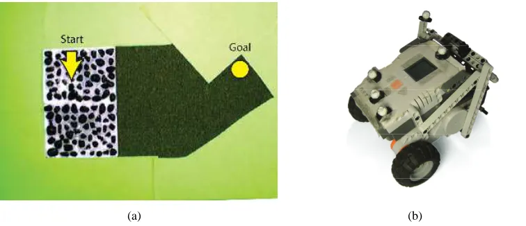
Our central hypothesis is that offset dynamics are a simple model that reasonably approximate several real world scenarios. In our third experiment, we applied our algorithm to a simulated problem using in which an agent needs to learn the best route to drive to work, and used date collected from real cars to simulate the dynamics. In our final experiment we applied our algorithm to a real-world robot car task in which the car most cross varying terrain (carpet and rocks) to reach a goal location.

CORL requires a planner to solve the estimated state MDP. Planning in continuous-state MDPs is an active area of research in its own right, and is known to be provably hard (Chow and Tsitsiklis, 1989). In all our experiments we used a standard technique, Fitted Value Iteration (FVI), to approximately solve the current MDP. In FVI, the value function is represented explicitly at only a fixed set of states. In our experiments these fixed states are uniformly spaced in a grid over the state space. Planning requires performing Bellman backups for each grid point; the value function over points not in this set is computed by function interpolation. We used Gaussian kernel functions as the interpolation method. Using sufficiently small kernel widths relative to the spacing of the grid points will make the approach equivalent to using a nearest neighbour standard discretization. However, there are some practical advantages in coarse grids to more smooth methods of interpolation. We discuss this issue in more depth in the next section.

In each experiment, Nat was tuned based on informal experimentation.

4.1 Puddle World

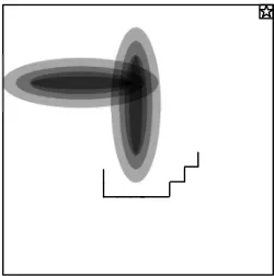
Puddle world is a standard continuous-state reinforcement-learning problem introduced by Boyan and Moore (1995). The domain is a two-dimensional square of width 1 with two oval puddles, which consist of the area of radius 0.1 around two line segments, one from(0.1,0.75)to(0.45,0.75)and the other from(0.45,0.4)to(0.45,0.8). The action space consists of the four cardinal directions. Upon taking an action the agent moves 0.05 in the specified cardinal direction with added Gaussian noise

N

(0,0.001_∗I), where I is a two-by-two identity matrix. The episode terminates when the agent reaches the goal region which is defined as the area in which x+y_≥1.9. All actions receive a reward of₋1 unless the agent is inside a puddle, in which case it then receives a reward of₋400 times the distance inside the puddle. Figure 1 provides a graphical depiction of the puddle world environment.

Figure 1: Puddle world. The small square with a star in it denotes the goal region. The black ovals represent the puddles and the black line represents a sample partial trajectory of an agent navigating around this world.

is only a single type, so CORL must learn only 4 sets of transition parameters, one for each action. Our goal here is simply to demonstrate that this additional information can lead to significantly faster learning over other more general techniques.

Puddle world has previously been used in reinforcement-learning competitions, and our eval-uation follows the procedure of the second bakeoff (Dutech et al., 2005). We initially generated 50 starting locations, and cycled through these when initializing each episode. Each episode goes until the agent reaches the goal, or has taken 300 actions. We report results from taking the av-erage reward within fifty sequential episodes (so the first point is the avav-erage reward of episodes 1-50, the second point is the average of episodes 51-100, etc.). We set Nat to be 15, and solved the

approximate MDP model using Fitted Value Iteration with Gaussian kernel functions. The kernel means were spaced uniformly in a 20x20 grid across the state space (every 0.05 units), and their standard deviation was set to 0.01. Note that in the limit as the standard deviation goes to 0 the func-tion interpolafunc-tion becomes equivalent to nearest neighbour. Nearest neighbour is the interpolafunc-tion method used in the approximate continuous-state MDP solver by Chow and Tsitsiklis (1991) which provides guarantees on the resulting value function approximation. However, since computational complexity scales exponentially with the grid discretization, practical application can require the use of coarse grids. In this case, we found that using a smoother function interpolation method empiri-cally outperformed a nearest neighbour approach. In particular, we found that a kernel width, which is a measure of the standard deviation, of 0.01 gave the best empirical performance. This value lies in the middle of kernel widths which are smaller than the variance of the dynamics models and the grid spacing and those widths larger than the grid spacing and dynamics models.

We compare our results to the reported results of Jong and Stone (2007)’s Fitted R-max and to Lagoudakis and Parr (2003)’s Least Squares Policy Iteration (LSPI).7Fitted R-max is an instance-based approach that smoothly interpolates the dynamics of unknown states with previously observed transitions, and takes a similar approach for modeling the reward function. LSPI is a policy iteration approach which uses a linear basis function representation of the state-action values, and uses a set of sample transitions to compute the state-action values.

Algorithm Number of episodes 50 100 200 400 CORL ₋19.9 ₋18.4 ₋20.3 ₋18.7 Fitted R-max −130 −20 20 −20 LSPI ₋500 ₋330 ₋310 ₋80

Table 1: PuddleWorld results. Each entry is the average reward/episode received during the prior 50 episodes. Results for the other algorithms are as reported by Jong and Stone (2007).

On the first 50 episodes, Fitted R-max had an average reward of approximately₋130, though on the next 50 episodes it had learnt sufficiently good models that it reached its asymptotic performance of an average reward of approximately₋20. In contrast, CORL learned a good model of the world dynamics within the very first episode, since it has the advantage of knowing that the dynamics across the entire state space are the same. This meant that CORL performed well on all subsequent episodes, leading to an average reward on the first 50 episodes of ₋19.9. Least Squares Policy Iteration (Lagoudakis and Parr, 2003) learned slower than Fitted R-max. Results are summarized in Table 1.

It is worth a short remark on the comparability of the reported results, as LSPI and Fitted R-max were run without knowing the reward model. LSPI’s performance on a deterministic reward reinforcement-learning problem such as PuddleWorld will be identical to its performance in the known-reward case, as the rewards in the sampled transitions will be the same in either situation. Given this, assuming known reward, as we do for CORL, will not change the LSPI results. In contrast we do expect that Fitted R-max will be slightly faster if it does not have to learn the reward model. This is because a wider interpolation width can be selected if the reward is known and only the dynamics are unknown, since all states share the same dynamics. However, even in this case, Fitted R-max will be approximating the Gaussian dynamics by a set of observed transitions, and so it appears likely that CORL will still be faster than Fitted R-max since CORL assumes the (true) parametric representation of the transition model.

In summary, given the reward function, CORL can learn a good dynamics model extremely quickly in PuddleWorld, since the dynamics are typed-offset with a single type. This additional information enables CORL to learn a good policy for puddle world much faster than Fitted R-max and LSPI. This experiment illustrates the advantage of CORL when the transition dynamics are known to be identical across the state space, and to follow a noisy offset model.

4.2 Catching a Plane

Figure 2: Motivating example where an agent must drive from a start location (designated with an S) to a goal area (shown with a highlighted rectangle) in time for a deadline, and can choose to take large high speed and variance roads, or slower small variance roads.

In our first experiment we considered a scenario in which learning this variance is critical: an agent must learn the best way to drive to an airport in time to catch a plane. A similar real-world environment is depicted in Figure 2. The agent starts from home and can either drive directly along a small side street, or cross over to the left or right to reach a main highway. The agent goes forward more quickly on the highway (with a mean offset of 2 units), but the highway also has a high variance of 0.49. In contrast, on the small side streets the agent goes forward more slowly (a mean offset of 1 unit) but with very small variance (0.00001). The state space is four dimensional, consisting of the agent’s current x and y location, its orientation, and the amount of time that has passed. On each step five minutes pass. The agent can drive in a 14 by 19 region: outside of this is considered to be too far away.8If the agent exits this region it receives a reward of₋1. The cost for each step is₋0.05, the reward for reaching the airport in time for check in is+1 and the cost for not making the airport in time is₋1. The discount factor is set to 1.0. Natwas set to 10. An episode

starts when the agent takes its first step and lasts until the agent reaches the goal, exits the allowed region, or reaches the time at which check in for the plane closes. The agent starts at location 7,3 facing north, and must figure out a way to reach the goal region which spans[6.5₋8.5,15.5-17.5]. To solve the underlying MDP, fitted value iteration was used. The fixed points were regularly spaced grid points with 15 across the x dimension, 20 across the y dimension, 4 orientation angles, and 21 time intervals. This yielded over 25,000 fixed points.

The correct path to take depends on the amount of time left. Here we explored three different deadline scenarios: when the agent has 60 minutes remaining (RunningLate), 70 minutes remaining (JustEnough), or 90 minutes remaining until check in closes for the plane (RunningEarly). In all three scenarios, the agent learned a good enough model of the dynamics within 15 episodes to compute a good policy. Note that using a na¨ıve discretization of the space with the FVI fixed points as states and applying R-max would be completely intractable, as a different model would have to be learned for each of over 25,000 states. We display results for all three scenarios in Table 2. In

15 0,0

20

(a)

15 0,0

20

Road 1

Road 2

Road 3

Work

(b) (c)

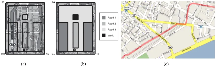
Figure 3: (a) Simulated world map showing example environment. (b) World divided into a set of discrete types. Agent starts at driveway (black circle) and tries to learn a good route to reach work. (c) An example section of a car trajectory (constructed from a set of GPS locations).

the RunningLate scenario the agent learned that the side streets are too slow to allow it to ever reach the airport in time. Instead it took the higher variance highway which enables it to reach the airport in time in over half the episodes after Nat is reached for all types: its average reward is−0.4833

and it takes on average 56.62 minutes for it to reach the airport. In JustEnough the agent learned that the speed of side streets is sufficiently fast for the agent to reach the airport consistently in time, whereas the higher speed and variance highway would result in the agent failing to reach the check in time in some cases. Here the agent always reached the goal and receives an average reward of 0.45. In the RunningEarly scenario, the agent has enough time so that it can take either route and reliably reach the airport in time. In this scenario it learned to always take the highway, since in expectation that route will be faster. The average reward here was 0.4629.

This simulation serves to illustrate that our algorithm can quickly learn to perform well, in situations in which learning the variance is critical to ensure good performance.

4.3 Driving to Work

In our second experiment we again consider a simulated trip routing problem, but we now generate transitions in the simulator by sampling from real traffic data distributions. Here an agent must learn the best series of actions to drive from home to work in a small simulated world (see Figure 3(a) and 3(b)). The state consists of the current coordinates(x,y)and the orientation of the agent. There are three road types and each road type is associated with a different distribution of speeds. The

Scenario Deadline (min) Mean Reward/Episode Mean Time to Reach Goal (min)

RunningLate 60 ₋0.4833 56.62

JustEnough 70 0.45 60

RunningEarly 90 0.4629 58.6

−2 −1 0 1 2 3 4 0

0.1 0.2 0.3 0.4 0.5

Transition Offset

Probability

Empirical distribution Estimated noisy offset model

Figure 4: A histogram of car speeds on small roads that is used to generate transitions on road type 2 and the estimated dynamics model parameters found during the experiment

distributions were obtained from the CarTel project (Eriksson et al., 2008), which consists of a set of car trajectories from the Boston, Massachusetts area. GPS locations and time stamps are stored approximately every second from a fleet of 27 cars.9 A section from one car trajectory is shown in Figure 3(c). Using this data set we extracted car trajectories on an interstate highway, small side streets and a local highway: these constitute types 1, 2 and 3 respectively in the simulation world. Each car trajectory consisted of a set of D GPS+time data points, which was converted into a set of D₋1 transitions. Each transition in the simulation was sampled from these world transitions; for example, transitions in the simulator on road type 2 were sampled from real-world transitions on small side streets. Transitions from all three road types were all rescaled by the same constant in order to make the distances reasonable for the simulated world.10 _{Figure 4} displays a histogram of rescaled transitions associated with small side streets. This figure shows that the speed distribution for small side streets was not Gaussian: the speed distribution for the other two street types was also not Gaussian. In particular, in no trajectories used does the car ever go backwards, whereas in some Gaussian models there will be small probability of this occurring. In this experiment we sought to investigate how well a noisy offset model could function in this environment, and the benefit of directly modelling different types of roads. Each transition in the simulated environment was sampled from the histogram of speeds associated with the road type at the agent’s current position. Therefore, the data from the simulator is closer to the real environment than to the Gaussian distributions assumed by the learning algorithm.

The agent received a reward of 1 for reaching the work parking lot, ₋0.05 for each step, and

−1 if it left the local area. Each episode finished when the agent either reached the goal, left the local area, or had taken 100 steps. An agent can go left, right or straight at each step. The transition induced by a straight action was determined by the road type as specified in the prior paragraph, and going left or right changed the orientation of the agent by 90 degrees with a very small amount of noise. The number of samples needed until a type-action tuple is known, Nat, was set to be 20.

The discount factor was 1. The agent was always started in the same location and was allowed to learn across a set of 50 episodes. Results were averaged across 20 rounds of 50 episodes per

9. See more information about the project athttp://cartel.csail.mit.edu/.