Hybrid Pattern Recognition and Multi-resolution Analysis (MRA) Based Fault Location in Power Transmission Lines

(1)

_____________________________________________________________________________________________________

Hybrid Pattern Recognition and Multi-resolution

Analysis (MRA) Based Fault Location in Power

Transmission Lines

Jude I. Aneke

1*

, O. A. Ezechukwu

1

and P. I. Tagboh

2

1_{Nnamdi Azikiwe University, Awka, Nigeria.}

2_{Electronic Development Institute, Awka, Nigeria.}

Authors’ contributions

This work was carried out in collaboration among all authors. All authors read and approved the final manuscript.

Article Information

DOI: 10.9734/JERR/2019/v8i416998 Editor(s): (1) Dr. P. Elangovan, Faculty of Electrical Engineering, Sri Venkateswara College of Engineering, Anna University, Chennai,

India. (2)Dr. Anuj Kumar Goel, Professor, CMR Engineering College, Kandlakoya (V), India. Reviewers: (1) Hachimenum Amadi, Federal University of Technology, Nigeria. (2)Raheel Muzzammel, University of Lahore, Pakistan. (3)Rajendra Prasad Payasi, KNIT, India. Complete Peer review History:http://www.sdiarticle4.com/review-history/44043

Received 02 April 2019 Accepted 11 June 2019 Published 05 December 2019

ABSTRACT

This paper proposes a fault (line-to-line) location on Ikeja West – Benin 330kV electric power transmission lines using wavelet multi-resolution analysis and neural networks pattern recognition abilities. Three-phase line-to-line current and voltage waveforms measured during the occurrence of a fault in the power transmission-line were pre-processed first and then decomposed using wavelet multi-resolution analysis to obtain the high-frequency details and low-frequency approximations. The patterns formed based on high-frequency signal components were arranged as inputs of the neural network, whose task is to indicate the occurrence of a fault on the lines. The patterns formed using low-frequency approximations were arranged as inputs of the second neural network, whose task is to indicate the exact fault type. The new method uses both low and high-frequency information of the fault signal to achieve an exact location of the fault. The neural network was trained to recognize patterns, classify data and forecast future events. Feed forward networks have been employed along with back propagation algorithm for each of the three phases

(2)

Jude et al.; JERR, 8(4): 1-14, 2019; Article no.JERR.44043

in the Fault location process. An analysis of the learning and generalization characteristics of elements in power system was carried using Neural Network toolbox in MATLAB/SIMULINK environment. Simulation results obtained demonstrate that neural network pattern recognition and wavelet multi-resolution analysis approach are efficient in identifying and locating faults on transmission lines as the average percentage error in fault location was just 0.1386%. This showed that satisfactory performance was achieved especially when compared to the conventional methods such as impedance and travelling wave methods.

Keywords: Pattern recognition; feed forward back propagation algorithm; neural network; Levenberg-Marquardt algorithm; power system protection.

1. INTRODUCTION

Transmission lines constitute the major part of the electric power system. Transmission and distribution lines are vital links between the generating unit and consumers to achieve the continuity of electric supply. To economically transfer large blocks of power between systems and from remote generating sites, High Voltage (HV) and Extra high voltage (EHV) overhead transmission systems are being used. Transmission lines also form a link in interconnected system operation for bi-directional flow of power [1]. Transmission lines run over hundreds of kilometres to supply electrical power to the consumers. They are exposed to the atmosphere and environmental hazards, hence chances of occurrence of fault in a transmission line is very high which when they eventually occur has to be immediately detected, located and cleared in order to minimize damage caused by it [2].

Having an effective automated means of identifying and determining the location of the fault even right from the control-room will significantly improve continuity of power supply. It will also facilitate quicker repair, improve system availability and performance, reduce operating cost and save time and effort of maintenance crew searching in, sometimes in

harsh environmental conditions. It has always been an interest for engineers to detect

and locate the faults in the power system as early as possible [3]. Fast clearing and restoration is very essential as it not only provides reliability but sometimes also stops the propagation of disturbances which may lead to blackouts.

2. MATERIALS AND METHODS

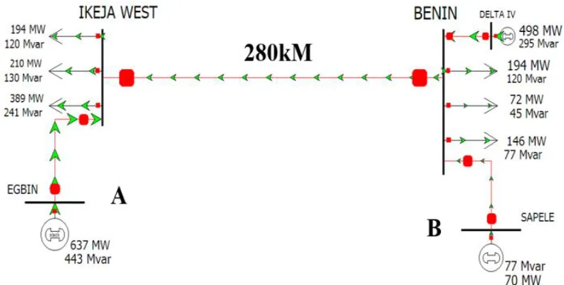
The Nigerian 330kV Ikeja West - Benin transmission line system was adopted and used to develop and implement the proposed

strategy using ANN. Fig. 1 shows a Power World Simulator one-line diagram (in run mode) of the system that has been used in this paper. The system consists of three

generators of 330kV each located on either end of the transmission line. The transmission line has been modelled using distributed parameters [4] so that it more accurately describes a very long transmission line.

This power system was remodelled and simulated using the Sim Power Systems toolbox in Simulink with the help of Math Works (R2016a). A snapshot of the model used for obtaining the training and test data sets is shown in Fig. 2. In Fig. 2, Z1 and Z2 are the source impedance of the generators on either side. A three-phase fault simulator used to simulate faults at various positions on the transmission line. The three-phase V-I measurement block is used to measure the

voltage and current samples at the terminal A. The transmission line (line 1 and line 2

together) is 280 km long and the three- phase fault simulator is used to simulate double line fault at varying locations along the transmission line with different fault

resistances.

2.1 Data Acquisition and Pre-processing

(3)

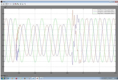
measured at 140kM away from source A during the occurrence of a fault on the line. The red, blue and green curves represent fault conditions of phases A, B and C respectively. From the

graphs, it can be seen that the transient fault occurred at 16.7ms and the system regained stability after 83.33ms.

Fig. 1. One-line diagram of the Nigerian 330 kV Ikeja West - Benin transmission line system (the studied system)

(4)

Fig. 3. Current waveform of line - line fault on phases A & B at a distance of 140 km from the source

(5)

2.2 Discrete Wavelet Transform

The application of wavelet transform in engineering areas usually requires a discrete wavelet transform (DWT). Here, the discrete form of the values r, k, a, , and ( ) will now be j, s, w, n and ( ) respectively. The representation of DWT can be written as [6]:

∅( , ) =_√ ∑ ( )∅ , ( ) (1)

≥

( , ) =

√ ∑ ( ) , ( ) (2)

Where, ( ) is the discrete signal to be decomposed, 1

√ is a normalizing factor. (1)

and (2) are the scaling function and the wavelet transform respectively. Normally, if is fixed at zero (0), M is selected to be 2 ; = 2 and summation is performed up to j = 0, 1, 2, …, J-1, then the discrete form of the wavelet function

, is now;

, ( ) = 2 (2 − ) (3)

Putting _, ( ) into (2) gives

( , ) =

√ ∑ ( ) ∗ 2 (2 − ) (4)

But we have that the relationship between the scaling function and the discrete wavelet function is given by,

( ) = ∑ ℎ ( )√2 ∗ ∅(2 − ) (5)

Where, is the shift parameter, n is the scaling parameter and ℎ is a highpass filter.

To get (2 − ), (5) can be written as

(2 − ) = ∑ ℎ ( )√2 ∗ ∅(2(2 − ) − )

(6)

Let = − 2 , then = + 2

Then,

(2 − ) = ∑ ℎ ( − 2 )√2 ∗ ∅(2 − )

(7)

Putting (6) into (3) gives;

( , ) = 1

√ ( ) ∗ 2

∗ ℎ ( − 2 )√2 ∗ ∅(2 − )

Interchanging the summation order gives;

( , ) = ∑ ℎ ( − 2 )

√ ∑ ( ) ∗ 2 √2 ∗

∅(2 +1 − ) (8)

Relating (5) with (8);

∅( + 1, ) =

1

√ ( ) ∗ 2 √2 ∗ ∅(2 − )

Therefore,

( , ) = ∑ ℎ ( − 2 ) _∅( + 1, ) (9)

In very similar way, can be obtained;

∅( , ) = ∑ ℎ∅( − 2 ) ∅( + 1, ) (10)

The implication of (9) and (10) is that a scaling function, ∅( + 1, ) is being convolved with a highpass analysis filter ℎ ( − 2 ) to yield the detail information and low pass analysis filter

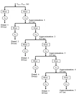
ℎ∅( − 2 ) to yield the coarse approximations respectively. This decomposition of the signal by successive high pass and low pass filtering of the time domain signal is called multi-resolution analysis (mra). In a block diagram, up to fifth level, it is represented as shown in Fig. 5.

The discrete wavelet transform (DWT)

represents a 1-D signal ( ) in terms of shifted versions of a low pass scaling function and shifted and dilated versions of a prototype band pass wavelet function [7].

Having converted the continuous signals into discrete signals, the sampled signals, _∅( + 1, ) are passed through a high pass filter

ℎ ( − 2 ) and a low pass filter ℎ∅( − 2 ). A process called wavelet decomposition using multi-resolution analysis. Then the outputs from both filters are decimated by 2 to obtain the detail coefficients and the approximation coefficients at level 1 (D1 and A1) [8]. The approximation coefficients are then sent to the

second stage to repeat the procedure. Finally, the signal is decomposed at the

(6)

Fig. 5. Fifthlevel multi-resolution analysis (MRA) representation of 2.3 Decomposition of the Signals

( ) Using Multi-resolution

Tool of Wavelet Transform

In order to reduce the computational burden, the sampling frequency should not be too high but it should be high enough to capture all the information concerning the faults. By randomly shifting the point of fault on the transmission line, number of simulations was carried out [9-10]. The generated current signal for each case is analyzed using wavelet transform. A sampling frequency of 10 kHz is selected. Daubechies wavelet Db5 is used as mother wavelet since it has good performance results for power system fault analysis. Detail coefficients of fault current signal in 5th level (d5), gives the frequency components corresponding to second and third

harmonics. On this basis, the summation of 5th level detail coefficients of the three-phase currents I , I and I are being used for the purpose of detection and classification of faults in the transmission line.

(7)

input to the respective neural networks for identification, classification and location.

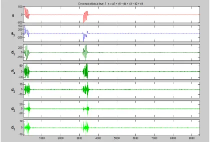
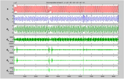
Figs. 6 and 7 show the wavelet decomposition of the Simulink extracted faulty waveforms of Figs. 3 and 4 respectively via multi-resolution analysis. The sampling frequency is 10kHz, the signal information captured by D1 is between 2.5kHz and 5kHz of the frequency band. D2 captures the information between 0.125 kHz and 0.25 kHz. D3 captures the information between 0.0625kHz and 0.125 kHz, and A3 retains the rest of the information of the original signal between 0 and 0.0625kHz. By such means, we can easily extract useful information from the original signal into different frequency bands and at the same time the information is matched to the related time period.

Fig. 6 depicts the snapshot of the fifth level decomposition of the sampled current waveforms of LL fault on phase A and B (of Fig. 3). , , , , and represent the detail coefficients for levels 1, 2, 3, 4, and 5 respectively while is the fifth level approximation coefficient. As clearly shown, the

three phases are concatenated together of matric data of 9420x3 in all. The first set of data of 3140x1 in a column is for phase A, the second set of data of 3140x1 is for phase B and the third set of data of 3140x1 is for phase C. The information of the original signal is clearly represented at each frequency band.

The snapshot of the fifth level decomposition of the sampled voltage waveforms of LL fault on phase A and B (of Fig. 4) is depicted in Fig. 7. , , , , and represent the detail coefficients for levels 1, 2, 3, 4, and 5 respectively while is the fifth level approximation coefficient. As clearly shown, the three phases are concatenated together of matric data of 9420x3 in all. The first set of data of 3140x1 in a column is for phase A, the second set of data of 3140x1 is for phase B and the third set of data of 3140x1 is for phase C. The information of the original signal is clearly represented at each frequency band.

The wavelet toolbox in MATLAB was used for the above signal decompositions as it provides a lot of useful techniques for wavelet analysis.

(8)

Fig. 7. Decomposed waveform of voltage waveform of LL Fault on phase A at a distance of 140 km from the source

3. RESULTS AND DISCUSSION

The design, development and performance of neural networks for the purpose of Line–Line fault location are discussed in this section. Once we can detect the occurrence of a fault on a transmission line and also classify the fault into the various fault categories [11-12], the next step is to pin-point the location of the fault from either end of the transmission line. Three possible line – line faults exist (A-B, B-C, C-A), corresponding to each of the three phases (A, B or C) being faulted.

3.1 Simulation Results of Training the Neural Network for Line – Line Fault Location

Feedforward back – propagation neural networks have been surveyed for the purpose of line – line fault location, mainly because of the availability of sufficient data to train the network. In order to train the neural network, several line – line faults have been simulated on the transmission line model. For each pair formed by the three phases, faults have been simulated at every 15 km on a 280 km long transmission line.

Along with the fault distance, the fault resistance has been varied as 0.25, 0.5, 0.75, 1, 5, 10, 20, 25, 50and 60 ohms respectively. Hence, a total of 1900 cases have been simulated (190 for each of the three phases with each of the ten different fault resistances). In each of these cases, the summed-up detail and approximation coefficients ( , , and ) of the fault currents of the three phases, are given as inputs to the neural network. The output of the neural network is the distance to the fault from terminal A. Hence, each input-output pair consists of three inputs and one output. An exhaustive survey on various neural networks has been performed by varying the number of hidden layers and the number of neurons per hidden layer. Of these ANNs, the most appropriate ANN is chosen based on its Mean Square Error performance and the Regression coefficient of the Outputs versus Targets.

(9)

network is 6.4741e-3 which is below the Cross-Entropy goal of 1e-2. It was found that the

correlation coefficient between the outputs and the targets was 0.99648 for this neural network.

Fig. 8. Mean square error performance of the ANN with configuration (3.12.5.15.30.1)

(10)

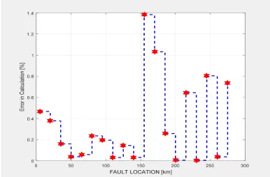
In order to test the performance of this network, 100 different phase to phase faults have been simulated on different phases with the fault distance being incremented by 15 kM in each case and the percentage error in calculated output has been calculated. Fig. 9 shows the results of this test conducted on the neural network (3.12.5.15.30.1). It can be seen that the maximum error is around 1.37% which is very satisfactory. The minimum error recorded was 0.08%. It is to be noted that the average error in the fault location is just 0.97 percent. Hence, this neural network has been chosen as the ideal network for the purpose of line – line fault location on transmission lines.

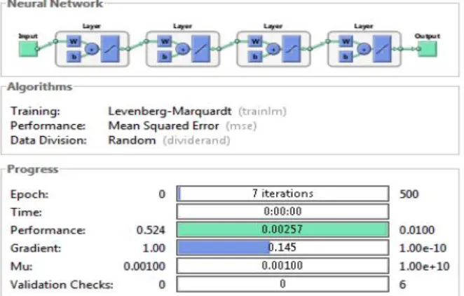
Fig. 10 provides an overview of the neural network and it is a screenshot of the training window simulated using the Artificial Neural Network Toolbox in Simu link. It is to be noted that the training process converged in about 55 iterations. It can be seen that the mean square error in fault detection achieved by the end of the training process was 2.57e-3 and that the number of validation check fails were zero by the end of the training process.

Fig. 11 plots the best linear regression fit between the outputs and the targets. The correlation coefficient (r) is a measure of how well the neural network’s targets can track the variations in the outputs (0 being no correlation at all and 1 being complete correlation). The

correlation coefficient, in this case, has been found to be 0.99648 which indicates excellent correlation (regression fit). The dotted line in the figure indicates the ideal regression fit and the red solid line indicates the actual fit of the neural network. It can be seen that both these lines track each other very closely which is an indication of very good performance by the neural network.

3.2 Simulation Results of Testing the Neural Network for Line – Line Fault Location

Several factors have been considered while testing the performance of the chosen neural network. One prime factor that evaluates the efficiency of the ANN is the test phase performance plot which is already illustrated in Fig. 9. As already mentioned, the average and the maximum error percentages are intolerable ranges and hence the network's performance is considered satisfactory.

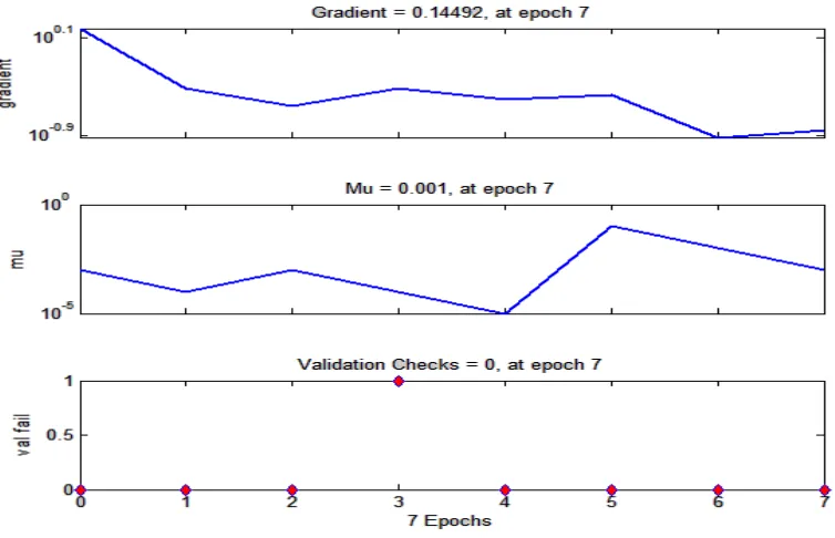
Fig. 12 provides another means of evaluating the ANN, which is the gradient and validation performance plot. It can be seen that there is a steady decrease in the gradient and also that the number of validation fails did not exceed 1 during the entire process which indicates smooth and efficient training because the validation and the test phases reached the Cross-Entropy goal at the same time approximately.

(11)

Fig. 11. Regression fit of the outputs versus targets with configuration (3.12.5.15.30.1)

Fig. 12. Gradient and validation performance plot of the ANN (3.12.5.15.30.1) The third factor that is considered while

evaluating the performance of the network is the correlation coefficient of each of the various phases of training, validation and testing. Fig. 13 shows the regression plots of the various phases

(12)

Fig. 14 shows the structure of the chosen ANN for line – line faults with 3neurons in the

input layer, 4 hidden layers with 12, 5, 15 and 30 neurons in them respectively and 1

neuron in the output layer (3.12.5.15.30.1). It is a pictorial representation of how the neurons in the respective layers are

connected together through the synaptic weights. It shows the interconnections between the input layer and the hidden layers, and also

between the hidden layers and the output layer. It can be seen that any given neuron is connected to all the neurons in the layer in front.

Table 1 illustrates the percentage errors in Fault location as a function of Fault Distance and Fault Resistance. Two different cases have been considered (shown in adjacent columns), one with a fault resistance of 15 ohms and another with a fault resistance of 70 ohms.

The measured fault locations are the mathematically calculated output of the trained chosen neural network after simulation in MATLAB environment using feed forward back-propagation algorithm.

It is to be noted that the resistance of 15 ohms was used as a part of the training data set and hence the average percentage error in fault location, in this case, is just 0.1386%. The second case illustrates the same with a different fault resistance of 70 ohms which is relatively very high and is not a part of the training set. Hence, the performance of the neural network, in this case, illustrates its ability to generalize and react upon new data. It is to be noted that the average error, in this case, is just 0.966% which is still very satisfactory. Thus, the neural networks performance is considered satisfactory and can be used for the purpose of line – line fault location.

(13)

Fig. 14. Structure of the chosen neural network (3.12.5.15.30.1)

Table 1. Percentage errors as a function of fault distance and fault resistance for the ANN chosen for line - line fault location

Serial no.

% Error vs. fault distance (Fault resistance = 15 Ω)

% Error vs. fault distance (Fault resistance = 70 Ω) Fault distance

(Km)

Measured fault location

% Error Fault distance (Km)

Measured fault location

% error

1 5 5.07 1.40 10 10.08 0.80

2 20 20.17 0.85 25 25.13 0.52

3 35 35.12 0.34 40 41.28 0.07

4 50 50.04 0.08 55 55.51 0.93

5 65 65.18 0.28 70 71.03 1.47

6 80 80.39 0.49 85 86.16 1.36

7 95 95.38 0.04 100 100.82 0.82

8 110 110.17 0.15 115 115.89 0.77

9 125 125.37 0.30 130 130.88 0.68

10 140 140.95 0.68 145 146.16 0.80

11 155 154.84 0.10 160 161.00 0.63

12 170 170.98 0.56 175 176.96 1.12

13 185 186.03 0.56 190 191.92 1.01

14 200 201.32 0.66 205 206.81 0.88

15 215 213.56 0.67 220 221.19 0.54

16 230 228.56 0.63 235 236.73 0.74

17 245 247.43 0.99 250 251.00 0.40

18 260 262.76 1.06 265 266.82 0.69

19 275 278.30 1.2 280 282.88 1.03

4. CONCLUSIONS

The paper has been able to successfully develop

a novel pattern recognition-based line-line fault location in an overhead transmission line

using the summation of the decomposed detail coefficients of the extracted faulty voltage

and current waveforms for all the three phases for ten different faults and also the non-fault case.

In summary, it can be deduced that it is very essential to investigate and analyze the advantages of a particular neural network structure and learning algorithm before choosing it for an application because there should be a trade-off between the training characteristics and the performance factors of any neural network.

(14)

an ideal transmission line fault location scheme especially in view of the increasing complexity of the modern power transmission systems. From simulation results, it can be also seen that back propagation neural networks are very efficient when a sufficiently large training data set is available and hence Back Propagation networks have been chosen for all the three steps in the fault location process.

Additionally, the case study network (Nigerian 330 kV Ikeja West – Benin Power Transmission line system) received for the first-time simulation results specific to its parameters.

COMPETING INTERESTS

Authors have declared that no competing interests exist.

REFERENCES

1. Das R, Novosel D. Review of fault location techniques for transmission and sub – transmission lines. Proceedings of 54th Annual Georgia Tech Protective Relaying Conference; 2000.

2. Amit MP, Abhijit SP. Fault location on transmission line using wavelet transform and Artificial neural network. IOSR Journal of Electrical and Electronics Engineering (IOSR-JEEE). 2016;11(4 Ver. II):59-62. [e-ISSN: 2278-1676, p-ISSN: 2320-3331] Available:www.iosrjournals.org

3. Girish PA, Nitin UG. Fault classification & location of series compensated trans-mission line using artificial neural network. International Journal of Advances in Electronics and Computer Science. 2015; 2(8).

[ISSN: 2393-2835]

4. Hasabe RP, Vaidya AP. Detection and classification of faults on 220 KV transmission line using wavelet transform and neural network. International Journal of Smart Grid and Clean Energy. 2014;3(3).

5. Suhaas Bhargava Ayyagari. Artificial neural network based fault location for

transmission lines. University of Kentucky Master’s Theses. 2011;657.

Available:http://uknowledge.uky.edu/grads chool_theses/657

6. Kale VS, Bhide SR, Bedekar PP, Mohan GVK. Detection and classification of faults on parallel transmission lines using wavelet transform and neural network. World Academy of Science, Engineering and Technology. 2008;22.

7. Jain A, Kale VS, Thoke AS. Application of artificial neural network to transmission line faulty phase selection and fault distance location. Proc. of IASTED Inter-national Energy and Power System Conf. 2006;262-267.

8. Celli G, Marchesi M, Mocci F, Pilo F. Application of neural networks in power distribution systems diagnosis and control, Proc. UPEC'97, Manchester. 1997;523-526.

9. Cichocki A, Lobos T. Artificial neural networks for real-time estimation of basic waveforms of voltage and currents. IEEE Trans. on PAS, 2011;9(2):612-619. 10. Kasinathan Karthikeyan. Power system

faultdetectionandclassificationbywavelet transforms and adaptive resonance theory neural networks. University of Kentucky Master's Theses. 2007;452.

Available:http://uknowledge.uky.edu/grads chool_theses/452

11. Atul AK, Navita GP. Fault detection and fault classification of double circuit transmission line using artificial neural network. International Research Journal of Engineering and Technology (IRJET) e-ISSN: 2395 -0056. 2015;02(08).

Available:www.irjet.net [p-ISSN: 2395-0072]

12. Aurangzeb M, Crossley PA, Gale P. Fault location using high frequency travelling waves measured at a single location on transmission line. Proceedings of 7th International conference on Developments in Power System Protection – DPSP, IEE CP479. 2001;403-406.

© 2019 Jude et al.; This is an Open Access article distributed under the terms of the Creative Commons Attribution License (http://creativecommons.org/licenses/by/4.0), which permits unrestricted use, distribution, and reproduction in any medium, provided the original work is properly cited.

Peer-review history: