Stable and Efficient Gaussian Process Calculations

Stable and Efficient Gaussian Process Calculations

Leslie Foster [email protected]

Alex Waagen [email protected]

Nabeela Aijaz NABBO [email protected]

Michael Hurley [email protected]

Apolonio Luis [email protected]

Joel Rinsky JOEL [email protected]

Chandrika Satyavolu CHANDRIKA [email protected]

Department of Mathematics San Jose State University San Jose, CA 95192, USA

Michael J. Way [email protected]

NASA Goddard Institute for Space Studies New York, NY, 10025, USA

Paul Gazis [email protected]

Ashok Srivastava [email protected]

NASA Ames Research Center

Intelligent Systems Division, MS 269-4 Moffett Field, CA 94035, USA

Editor: Chris Williams

Abstract

The use of Gaussian processes can be an effective approach to prediction in a supervised learning environment. For large data sets, the standard Gaussian process approach requires solving very large systems of linear equations and approximations are required for the calculations to be practi-cal. We will focus on the subset of regressors approximation technique. We will demonstrate that there can be numerical instabilities in a well known implementation of the technique. We discuss alternate implementations that have better numerical stability properties and can lead to better pre-dictions. Our results will be illustrated by looking at an application involving prediction of galaxy redshift from broadband spectrum data.

Keywords: Gaussian processes, low rank approximations, numerical stability, photometric red-shift, subset of regressors method

1. Introduction

have good numerical stability properties in the sense that the growth of computer arithmetic errors is limited.

The paper begins with a review of Gaussian processes and the subset of regressors approach. We then show that implementation of the subset of regressors method using normal equations can be inaccurate due to computer arithmetic errors. A key contribution of the paper is a discussion of alternative implementations of the subset of regressors technique that have improved numerical stability. Another valuable contribution of the paper is a discussion of how pivoting can be incor-porated in the subset of regressors approach to further enhance numerical stability. We discuss the algorithm of Lucas (2004, pp. 4-5) for construction of a partial Cholesky factorization with pivoting and emphasize that with this algorithm the flop count, including subset selection, of the subset of regressors calculations is O(nm2).

In Section 2 we provide background about using Gaussian processes to facilitate prediction. In Section 3 we discuss how low rank approximations lead to the subset of regressors approach. In Section 4 we describe why a commonly used implementation of this technique may suffer from numerical instabilities and in Section 5 we propose two alternative implementations that have better numerical stability properties. In Section 6 we address the subset selection problem and indicate that a solution to this problem can enhance numerical stability. In Section 7 we discuss tools that aid in the choice of rank in the low rank approximation. In Section 8 we illustrate that the numerical stability issues addressed in Section 4 can lead to unacceptably large growth of computer arithmetic errors in an important application involving prediction of galaxy redshift from broadband spectrum data. Our alternative implementations of the subset of regressors method overcome these difficulties. Also in Section 8 we discuss code, available at http://dashlink.arc.nasa.gov/algorithm/ stableGP, that implements our ideas. Finally, in Section 9 we summarize our results.

2. Gaussian Processes

Supervised learning is the problem of learning input-output mappings using empirical data. We will assume that a training data set is known consisting of a n_×d matrix X of input measurements and a n by 1 vector y of output or target values. The task is to use the training data set to develop a model

that can be used to make prediction with new data. We will assume the new data, called the testing data, is contained in an n∗_×d matrix X∗ of inputs. The n∗_×1 vector y∗will represent the target values corresponding to X∗. The goal is to predict the value of y∗given X , y, and X∗.

In the Gaussian process approach the prediction of y∗involves selection of a covariance function

k(x,x′), where x and x′are vectors with d components. It is required that the covariance function be positive semidefinite (Rasmussen and Williams, 2006, p. 80) which implies that the n_×n covariance

matrix K with entries Ki j=k(xi,xj)where xiand xjare rows of X is symmetric positive semidefinite

(SPS), so that vTKv_≥0 for any n_×1 real column vector v. The covariance function can be used to construct K and also the n∗ by n cross covariance matrix K∗where K_{i j}∗ =k(x∗_i,xj) where x∗i is the ithrow of X∗. The predictionby∗for y∗is given by the Gaussian processes equation (Rasmussen and Williams, 2006, p. 17):

b

y∗=K∗(λ2_I+K)−1_{y. (1)}

The parameterλin this equation represents the noise in the measurements of y and, in practice, it is often selected to improve the quality of the model (Rasmussen and Williams, 2006).

squared exponential (sometimes called the radial basis function), Matern, rational quadratic, neural network, polynomial or other covariance functions (Rasmussen and Williams, 2006, pp. 79-102). Most of these covariance functions contain free parameters that need to be selected. Such param-eters and λ in (1) are called hyperparameters. We will not focus on the choice of a covariance function or alternative methods for selection of hyperparameters in this paper. In the examples dis-cussed in Section 8 we tried out a variety of covariance functions and selected the one that provided the best predictions. Hyperparameters were selected using the Matlab routine minimize (Rasmussen and Williams, 2006, pp. 112-116, 221) which finds a (local) maximum of the marginal likelihood function calculated using the training set data.

We should mention that the choice of the hyperparameterλcan affect the numerical stability of the Gaussian process calculations. Generally larger values ofλlead to reduced computer arithmetic errors but a large value of λmay be a poor theoretical choice—note thatyb∗_→0 as λ_→∞. One needs to select a value of λ that balances such competing errors. The choice of λ in Gaussian processes is closely related to the parameter choice in ridge regression in the statistics literature (Montgomery et al., 2006, pp. 344-355) and in the literature on regularization (Hansen, 1998, pp. 175-208). As mentioned above we select hyperparameters, includingλ, using the routine minimize (Rasmussen and Williams, 2006, pp. 112-116, 221). This technique worked well for the practical example presented in Section 8 when used with our algorithms with improved numerical stability.

We should note that Gaussian process approach also leads to an equation for C the covariance matrix for the predictions in (1). If the n∗_×n∗matrix K∗∗has entries K_{i j}∗=k(x∗_i,x∗_j)then (Rasmussen and Williams, 2006, pp. 79-102):

C=K∗∗₋K∗(λI+K)−1_K∗T_{. (2)}

The superscript T indicates transpose. The pointwise variance of the predictions is diag(C), the diagonal of the n∗_×n∗matrix C.

3. Low Rank Approximation: The Subset of Regressors Method

In (1) the matrix(λ2_{I+K)is an n by n matrix that, in general, is dense (that is has few zero entries).}

Therefore for large n, for example n_≥10000, it is not practical to solve (1) since the memory required to store K is O(n2) and the number of floating point operations required to solve (1) is

O(n3). Therefore for large n it is useful to develop approximate solutions to (1). To do this, for some m<n, we can partition the matrices K and K∗as follows:

K=

K11 K12 K21 K22

= K1 K2,K∗= K₁∗ K₂∗. (3)

Here K11 is m×m, K21 is(n−m)×m, K12=K21T is m×(n−m), K22 is(n−m)×(n−m), K1 is n_×m, K2is n_×(n₋m), K₁∗is n∗_×m and K₂∗is n∗_×(n₋m). Next we approximate K and K∗using

K∼=Kb_≡K1K11−1K T

1 (4)

and

K∗∼=Kb∗_≡K₁∗K₁₁−1K₁T

and in (1) we replace K withK and Kb ∗withKb∗. Therefore

b

K₁∗K₁₁−1K₁T(λ2_I+K1K−1

11 K1T)−1y= K₁∗K₁₁−1(λ2I+K₁TK1K₁₁−1)−1K₁Ty, so that

b

y∗_N=K₁∗(λ2K11+K₁TK1)−1K₁Ty. (5) Equation (5) is called the subset of regressors method (Rasmussen and Williams, 2006, p. 176) and was proposed, for example, in Wahba (1990, p. 98) and Poggio and Girosi (1990, p. 1489). As we discuss in the next section the subscript N stands for normal equations. We refer to use of (5) as the SR-N approach.

If m<<n then (5) is substantially more efficient than (1). For large n the leading order term

in the operation count for the calculations in (5) is nm2 flops or floating point operations (where a floating point operation is either an addition, subtraction, multiplication or division), whereas the calculations in (1) require approximately 2n3/3 flops. If n=180,000 and m=500, as in an example discussed later, the solution to (1) requires approximately 4_×1015 flops which is five order of magnitudes greater than the approximately 4_×1010flops required to solve (5). Furthermore, to use (1) one needs to calculate all n2+nn∗elements of K and K∗whereas (5) requires that one calculate only the nm+n∗m elements in K1and K₁∗. This also improves the efficiency of the calculations and will reduce the memory requirements dramatically.

We should add that if in Equation (2) we use the approximations (4), (3) and

K∗∗∼=Kb∗∗_≡K₁∗K₁₁−1K₁∗T

then, in (2) replacing K withK, Kb ∗withKb∗, K∗∗withKb∗∗and using algebra similar to that used in deriving (5), it follows that

C∼=CNb _≡λ2K₁∗(λ2K11+K₁TK1)−1K₁∗T. (6) For an alternate derivation of (6) see Rasmussen and Williams (2006, p. 176). Also diag(C) ∼=

diag(CbN) so that diag(CbN) provides approximations for the variance of the predictions.

4. Numerical Instability

The sensitivity of a problem measures the growth of errors in the answer to the problem relative to perturbations in the initial data to the problem, assuming that that there are no errors in the solution other than the errors in the initial data. A particular algorithm implementing a solution to the problem is numerically stable if the error in the answer calculated by the algorithm using finite precision arithmetic is closely related (a modest multiple of) the error predicted by the sensitivity of the problem. An algorithm is unstable if the error in the answer calculated by the algorithm is substantially greater than the error predicted by the sensitivity of the problem.

A straightforward implementation for the subset of regressors approximation using (5) has a po-tential numerical instability. To see this note that since K is SPS it follows that the m_×m submatrix K11 is also. Therefore we can factor the matrix K11with a Cholesky factorization (Golub and Van

Loan, 1996, p. 148)

K11=V11V₁₁T (7)

where V11is an m×m lower triangular matrix. Now let A=

K1 λV₁₁T

and b=

y

0

where 0 is an m×1 zero vector, A is an(n+m)_×m matrix and b is a(n+m)_×1 vector. Consider the least square problem:

min

x ||Ax−b|| (9)

where the norm is the usual Euclidean norm. The normal equations solution (Golub and Van Loan, 1996, p. 237) to this least squares problem is x= (ATA)−1_AT_{b= (λ}2_V

11V11T+K1TK1)−1K1Ty and so

by (7)

xN= (λ2K11+K₁TK1)−1K₁Ty. (10) Therefore the solutionby∗_Npresented in (5) can also be written

b

y∗_N=K₁∗xN. (11)

The subscript N indicates the use of the normal equations solution to (8).

The potential difficulty with the above solution is that the intermediate result xN is the solution

to a least squares problem using the normal equation. It is well known that the use of the normal equation can, in some cases, introduce numerical instabilities and can be less accurate than alterna-tive approaches. As discussed in Golub and Van Loan (1996, p. 236-245) the sensitivity of the least squares problem (9) is roughly proportional to cond(A) +ρLScond2(A), whereρLS=||b−Ax||and

cond(A) =_||A_||||(ATA)−1_AT_{||is the condition number of A. The problem with the normal}

equa-tions solution to (9) is that the accuracy of the calculated solution is (almost always) proportional to cond2(A), the square of the condition number of A, whereas in the case that ρLS is small the

sensitivity of the least squares problem is approximately cond(A). To quote from Golub and Van Loan (1996, p. 245):

We may conclude that if ρLS is small and cond(A) is large, then the method of

normal equations. . . will usually render a least squares solution that is less accurate than a stable QR approach.

We will discuss use of the stable QR approach and another alternative to the normal equations in the next section.

5. Improving Numerical Stability

The calculation ofby∗_N as given by (5) is equivalent to the solution to (9) and (11) using the normal Equations (10). We can reduce the computer arithmetic errors in the calculation ofby∗_Nif we develop algorithms that avoid the use of the normal equations in the solution to (9) and (11) . We will present two alternative algorithms for solving (9) and (11). We should add that although these algorithms can have better numerical properties than use of (5), all the algorithms presented in this section are mathematically (in exact arithmetic) equivalent to (5).

5.1 The Subset of Regressors Using a QR Factorization

We first describe use of the QR factorization to solve (9). In this approach (Golub and Van Loan, 1996, p.239) one first factors A=QR where Q is an(n+m)_×m matrix with orthonormal columns

and R is an m_×m right triangular matrix. Then

xQ=R−1QTb=R−1QT

y

0

so that

b

y∗_Q=K₁∗xQ=K1∗R−1QT

y

0

. (13)

With the above algorithmby∗can still be solved quickly. Assuming that the elements of K1and K₁∗have been calculated, and that m<<n, then the approximate number of operations for the QR

approach is 2nm2 flops. Therefore both the QR and normal equations approach require O(nm2)

flops.

We should also note that we can use the QR factorization to reduce computer arithmetic errors in the computation of the approximate covariance matrix in (6). If we let

b

CQR≡λ2(K1∗R−1)(K1∗R−1)T

then mathematically (in exact arithmetic)CbN andCbQRare the same. However, for reasons similar to

those discussed in Section 4, the computer arithmetic errors inCQRb will usually be smaller than those inCNb , assuming, for example, thatCNb is computed using a Cholesky factorization ofλ2K11+K₁TK1. We will refer to the subset of regressors method using the QR factorization as the SR-Q method. We should add that the use of a QR factorization in equations related to Gaussian process calcula-tions is not new. For example Wahba (1990, p. 136) discusses using a QR factorization for cross validation calculations.

5.2 The V Method

If we assume the V11is nonsingular we can define the n×m matrix V :

V =K1V11−T (14)

where the superscript ₋T indicates inverse transpose. Note that by (7) it follows that V is lower

trapezoidal and that V=

V11 V21

, where V21=K21V11−T. Substituting K1=VV11T and (9) into (10) we

get

xV =V11−T(λ2I+VTV)−1VTy (15)

so that

b

y_V∗ =K₁∗xV =K1∗V11−T(λ

2_I+VT_V)−1_VT_{y. (16)}

We should note that this formulation of the subset of regressors method is not new. It is presented, for example, in Seeger et al. (2003) and Wahba (1990, p. 136) presents a formula closely related to (16). We will call the formula (16) forby∗the V method. We should note, as will be seen in Section 6.2, that one can calculate V as part of a partial Cholesky factorization rather than using (14).

We will see in our numerical experiments and the theoretical analysis in Section 6 that the V method is intermediate in terms of growth of computer arithmetic errors between the normal equations and QR approach. Often, but not always, the accuracy of the V method is close to that of the QR approach.

Assuming that the elements of K1 and K1∗ have been calculated, and that m<<n, then the

approximate number of operations for the V method is 2nm2 _{flops—approximately nm}2 _{flops to}

form V and another nm2 flops to solve for xV using (15). This is approximately the same as SR-Q

We can also compute the approximate covariance matrix with the V method approach:

b

CV ≡λ2K1∗V11−T(λ

2_I+VT_V)−1_V−1 11 K∗

T 1 .

In exact arithmeticCbN,CbQRandCbV are identical but the computer arithmetic errors are often smaller

inCbV andCbQRthanCbN.

5.3 Examples Illustrating Stability Results

We present two sets of examples that illustrate some of the above remarks.

Example 1 Let the n_×n matrices K be of the form K=U DUT where U is a random orthogo-nal matrix (Stewart, 1980) and D is a diagoorthogo-nal matrix with diagoorthogo-nal entries s1≥s2≥. . .sn≥0.

Therefore s1, s2,. . ., snare the singular values of K. We will choose a vector w_∈Rn, where Rnis real n dimensional space, of the form w=

x

0

where x_∈Rmis a random vector and 0 indicates a zero vector with(n₋m)components. We let the target data be y=Kw. We will also assume for simplicity thatλ=0.

Due to the structure of w each of xN (10), xQ(12), and xV (15) will calculate x exactly in exact arithmetic. Therefore in finite precision arithmetic_||x₋x˙_||, with ˙x = xN, xQor xV will be a measure of the computer arithmetic errors in the calculation.

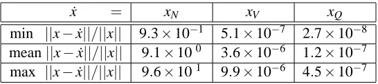
We carried out an experiment n=100, m=50, si=10−(i−1)/5, i=1,2, . . . ,m, and si=10−10, i=m+1,m+2, . . . ,n using a set of one hundred random matrices of this type. For this class of matrices the singular values of K vary between 1 and 10−10, cond(K) =1010and cond(K1)∼=1010. The results are:

˙

x = xN xV xQ

min _||x₋x˙_||/_||x_|| 9.3_×10−1 5.1_×10−7 2.7_×10−8 mean_||x₋x˙_||/_||x_|| 9.1_×100 3.6_×10−6 1.2_×10−7 max _||x₋x˙_||/_||x_|| 9.6_×101 9.9_×10−6 4.5_×10−7

Table 1: Min, mean and max errors,_||x₋x˙_||/_||x_||, for 100 matrices and various methods.

For this set of matrices xQand xV have small errors. However xNhas large errors due to its use of normal equations.

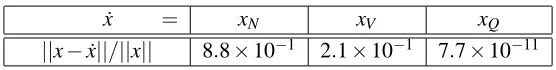
Example 2 This example will illustrate that, although the V method often greatly improves upon

the stability of the SR-N method, this is not always the case. For 0<s_≤1 let C=

s2 10s 10s 200

, let

the 4_×4 matrix K=

s2C 10sC 10sC 200C

, let x=

1/3 1/3

, w=



 x

0 0



,λ=0 let y=Kw.

˙

x = xN xV xQ

||x₋x˙_||/_||x_|| 8.8_×10−1 2.1_×10−1 7.7_×10−11 Table 2: Errors_||x₋x˙_||/_||x_||for a 4_×4 matrices and various methods.

In Section 6 and Appendix A we will discuss the reason that the V method performs poorly in this example and show that the numerical instability illustrated in this example can be cured by interchanging the columns and rows of K appropriately. Also we should note that although difficulties like the one illustrated here are possible for the V method, experiments like those in Example 1 suggest that such difficulties are not likely. As we discuss in Section 6, the method performed well when we applied it to real world applications.

6. Pivoting and Subset Selection

In Section 5 we discussed low rank approximations to K which involved the first m columns of

K. However one can select any subset of the columns to construct a low rank approximation. The

choice of these columns or the “active” set is the subset selection problem. This problem has been addressed by, for example, Smola and Bartlett (2001), Seeger et al. (2003), Csato and Opper (2002) and Fine and Scheinberg (2001). The technique that we will use is the same as that in Fine and Scheinberg (2001). However we will focus on the effect of the resulting choice of the active set on the numerical stability of the resulting algorithm. This is a different motivation than the motivations in the above references.

6.1 The Singular Value Decomposition

To pursue this we will first discuss the singular value decomposition which, in a certain sense, produces an optimal low rank approximation to K. The singular value decomposition (SVD) of the symmetric semidefinite matrix K produces the factorization

K=U DUT = U1 U2

D1 0 0 D2

U1 U2T

where U is an n_×n orthogonal matrix, D is an n_×n diagonal matrix whose diagonal entries s1≥ s2≥. . .≥sn≥0 are the singular values of K, U1is n×m, U2is n×(n−m), D1is an n×n diagonal

matrix, and D2is an(n−m)×(n−m)diagonal matrix. We then can construct the truncated singular

value decomposition (TSVD) low rank approximation to K:

b

KSV D=U1D1U₁T. (17)

The TSVD approximationKbSV Dis the best low rank approximation (Golub and Van Loan, 1996, p.

72) to K in the sense that

min

rank(Kb)=m||

K₋Kb_||=_||K₋KbSV D||=sm+1. (18)

generalizes to singular matrices the definition of condition number that we used in Section 4 (where

A had m columns). It then follows from (17) that

cond(KSV Db ) =s1/sm (19)

where s1and smare singular values of K (which are the same as the singular values ofKbSV D). Thus

the singular value decomposition provides two desirable properties:

• Equation (18) indicates thatKSV Db will be close to K, if there exists a rank m approximation that is close to K, and

• Equation (19) limits the condition number ofKbSV Dwhich will limit the growth of computer

arithmetic errors in the use ofKSV Db .

However, for large n, it is not practical to calculate the SVD of K since the SVD requires O(n3) oper-ations and is much more expensive than the algorithms described in Section 5 which require O(nm2)

operations. We would like to construct an approximation that requires only O(nm2)operations and that produces low rank approximations with properties related to (18) and (19).

6.2 Cholesky Factorization with Pivoting

The algorithms describe in Sections 3 and 5 (which are mathematically but not numerically identi-cal) do not satisfy relations related to (18) and (19) as is apparent from the following example.

Example 3 For the matrix

K= 



1+ε 1₋ε 0 1−ε 1+ε 0

0 0 1





if we let m=2 then by (4) and (17) we have

b K=

 

1+ε 1₋ε 0 1₋ε 1+ε 0

0 0 0



 andKbSV D=  

1 1 0

1 1 0

0 0 1

 

so that, for smallε,

||K₋KSV Db _||=2ε << 1=_||K₋Kb_||and

cond(KSV Db ) =2 << 1/ε=cond(Kb).

For this example the low rank approximationK has two problems: (1) it does not provide a goodb approximation to K even though a good low rank approximation exists and (2) the condition number ofK can be arbitrarily large which potentially could lead to a large growth of computer arithmeticb errors.

To overcome the difficulties illustrated in this example we can use a Cholesky factorization, with pivoting, to insure that linearly independent columns and rows appear first. The Cholesky factorization with pivoting produces a decompostion

where P is an n×n permutation matrix and L is an n×n lower triangular matrix. To produce our low

rank approximations to the Gaussian process equations we do not need to factor all of K, rather it is sufficient to calculate a partial factorization that factors only m columns and rows of PTKP. This is

a partial Cholesky factorization with pivoting. If the pivoting is done using complete pivoting (that is the pivoting in the Cholesky factorization is equivalent to using complete pivoting in Gaussian elimination) then there are a variety of algorithms that determine the factorization (Higham, 2002, p. 202; Golub and Van Loan, 1996, p. 149; Lucas, 2004, pp. 4-5 and Fine and Scheinberg, 2001, p. 255). Here we will summarize the algorithm presented in Lucas (2004, pp. 4-5) since it is not as widely known as the algorithms in Higham (2002, p. 202) and Golub and Van Loan (1996, p. 149) and is more efficient in our context. The algorithm below is also the same as that in Fine and Scheinberg (2001, p. 255) except for the stopping criteria.

Algorithm 1: Algorithm for the partial Cholesky factorization Data: an n_×n symmetric positive semidefinite matrix K

a stopping tolerance tol_≥0

the maximum rank, max rank_≤n, of the low rank approximation

Result: m, the rank of the low rank approximation an n_×m partial Cholesky factor V

a permutation vector piv

Note: on completion the first m rows and columns of PTKP₋VVT are zero, where P is a permutation matrix with Ppivi,i=1,i=1, . . . ,n

initialize:

di=Kii,i=1, . . . ,n

Kmax=maxi=1,...,n(di)

pivi=i,i=1, . . . ,n m=max rank

for j=1 to max rank do

[dmax,jmax] =maxi=j,...,n(di)

where jmaxis an index where the max is achieved

if dmax≤(tol)Kmaxthen m= j₋1 ;

exit the algorithm ; end

if jmax6= j then

switch elements j and jmaxof piv and d

for i= j+1 : n let ui=element i of column jmaxof PTKP

switch rows j and jmaxof the current n×(j−1)matrix V

end

Vj j=√dmax

for i= j+1 to n do

Vi j= (ui₋∑_kj−₌1₁VikVjk)/Vj j di=di₋V_{i j}2

There are two choices of the stopping tolerance tol that have been suggested elsewhere. For the choice tol=0 the algorithm will continue as long as the factorization determines that K is positive definite (numerically). This choice of tol is used in LINPACK’s routine xCHDC (Dongarra et al., 1979) and also by Matlab’s Cholesky factorization chol (which implements a Cholesky factorization without pivoting). The choice tol=n_×εwhereεis machine precision is suggested in Lucas (2004, p. 5) and in Higham (2002). The best choice of tol will depend on the application.

There are a number of attractive properties of the partial Cholesky factorization.

• The number of floating point operations in the algorithm is approximately nm2₋2m3/3 flops. The calculations to determine the pivoting require only O(nm)flops.

• The algorithm accesses only the diagonal entries of K and elements from m columns of K.

• The storage requirement for the algorithm is approximately n(m+2)floating point numbers plus storage for the integer vector piv and any storage needed to calculate entries in K.

• The accuracy and condition number of the low rank approximation to K produced by the algorithm is related to the accuracy and condition number of the low rank approximation produced by the singular value decomposition. In particular

Theorem 1 Let the n_×m matrix V be the partial Cholesky factor produced by Algorithm 1 and let

b

KP=PVVTPT. (20)

Also letKbSV D be the rank m approximation (17) produced by the singular value decomposi-tion. Then

||K₋KbP|| ≤c1||K−KbSV D||and (21)

cond(KbP)≤c2cond(KbSV D)where (22) c1≤(n−m)4mand c2≤(n−m)4m. (23)

Proof The theorem follows from results in Gu and Eisenstat (1996) for the QR factorization

with pivoting. First we consider a Cholesky factorization, without pivoting, of K so that K=LLT where L is and n_×n lower triangular matrix. Letσi(A)represent the ithsingular value of a matrix A. Then, making use of the singular value decomposition, it follows easily that σi(K) =σ2i(L), i=1, . . . ,n. Consider a QR factorization of LT with standard column pivoting (Golub and Van Loan, 1996, p. 249-250) so that QR=LTP1. The permutation matrix P1produced by this QR factorization will be identical, in exact arithmetic, to the permutation matrix produced by the Cholesky factorization with pivoting applied to K (Dongarra et al., 1979, p. 9.26). In addition, the Cholesky factorization, with pivoting, of K is P₁TKP1=RTR, assuming the diagonal entries of R are chosen to be nonnegative (Dongarra et al., 1979, p. 9.2). Now we partition the Cholesky factorization:

P₁TKP1=

RT₁₁ 0

RT₁₂ RT₂₂

R11 R12

0 R22

. (24)

It follows from Theorem 7.2 in Gu and Eisenstat (1996, p. 865) that

σ1(R22)≤c3σm+1(L)and

1

σm(R11) ≤ c4 1

σm(L)

Now the first m steps of Cholesky factorization, with pivoting, of K will produce identical results to the m steps of the partial Cholesky factorization described in Algorithm 1. Let

V =

V11 V21

and R1= R11 R12 so that RT₁ =

RT₁₁ RT₁₂

. (26)

In the (complete) Cholesky factorization with pivoting of K, after the first m steps of the algorithm additional pivoting will be restricted to the last n₋m rows and columns of PTKP. Let P2be a n×n permutation matrix representing the pivoting in the last n−m steps in the algorithm. Then it follows that

P1=PP2,V11=RT₁₁and RT₁ =P₂TV. Therefore

b

KP=PVVTP=P1P2TVVTP2P1T =P1RT1R1P1T. (27) By (18), (24), (25), (26) and (27) we can conclude that

||K₋KbP||=||RT22R22||=σ21(R22)≤c23σ2m+1(L) =c1σm+1(K) =c1||K−KbSV D||. Also, by (25), (27) and the interlace theorem (Bj¨orck, 1996, p. 15)

σm(KPb ) =σ2m(R1)≥σ2m(R11)≥σ2m(L)/c24=σm(K)/c24. (28) Next by (27) and the interlace theorem

σ1(KPb ) =σ21(R1)≤σ21(R) =σ1(K). (29) Finally, (19), (28) and (29) imply that

cond(KbP) =σ1(KbP)/σm(KbP)≤c24σ1(K)/σm(K) =c2cond(KbSV D).

The bounds in (23) on c1and c2grow exponentially in m and in principle can be large for larger

values of m. In practice this appears to be very uncommon. For example the constants c3and c4in

(25) are closely related to||W||where W =R−₁₁1R22 (Gu and Eisenstat, 1996, p. 865). Numerical experiments indicate the_||W_||is almost always small in practice (typically less than 10) (Higham, 2002, p. 207 and Higham, 1990). Therefore c1=c23 and c2=c24will not be large in practice. We

should add that there are choices of the pivot matrices P in (20) which guarantee bounds on c1and c2that are polynomials in n and m rather than exponential in m as in (23) (Gu and Miranian, 2004). However algorithms that produce such pivot matrices are more expensive than Algorithm 1 and, in practice, usually do not lead to an improvement in accuracy.

Prior to applying one of the methods—SR-N, SR-V and SR-Q—from Sections 3 and 5 one can carry out a partial Cholesky factorization of K to determine the permutation matrix P, and apply the algorithms of Sections 3 and 5 using the matricesKe_≡PT_KP,Ke∗_=K∗_{P and the vector} e

y=PTy. If pivoting is used in this manner, we will call the algorithms SR-NP, SR-VP and SR-QP

Since the algorithms SR-N, SR-V and SR-Q are all mathematically (in exact arithmetic) equiv-alent, then by (4) in all these algorithms the low rank approximation toK ise K1eKe₁₁−1Ke₁T whereK1e is the first m columns ofK ande Ke11is the first m rows ofKe1. Therefore the low rank approximation to K=PKPe T would be

b

KP=PK1eK11e Ke₁TPT. (30) We then have

Theorem 2 In exact arithmetic the matricesKPb in (20) and (30) are the same.

Proof Let V be the factor produced by a partial Cholesky factorization, with pivoting, of K. Then, as

mentioned in Algorithm 1, the first m columns and rows of PT_KP−VVT _{are zero. SinceKe=P}T_KP it follows thatK11e =V11V₁₁T andK1e =VV₁₁T, where V11 is the m×m leading principle submatrix of V . Therefore that VVT=Ke1Ke11−1Ke1T. We conclude PVVTPT=PKe1Ke11−1Ke1TPT.

A key conclusion of Theorems 1 and 2 is that for the algorithms SR-NP, SR-VP and SR-QP which use pivoting, the low rank approximationKbPto K has the desirable properties (21-23) which show

that the accuracy and condition number ofKPb is comparable to the accuracy and condition number of the low rank approximation produced by the singular value decomposition. Therefore if m is small, difficulties such as those illustrated in Example 3 are not possible since for small m the bound(n−m)4mfor c1 and c2 is not large. Furthermore, such difficulties are unlikely for large m

since, as mentioned earlier, for large m, the values of c1and c2are, apparently, not large in practice.

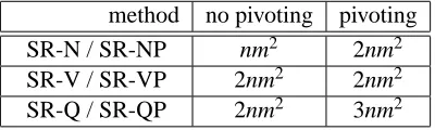
For the algorithm SR-VP one does not need to calculate V using (14) since, as shown in the proof of Theorem 2, V is calculated by the partial Cholesky factorization. Using this fact the floating point operation counts of the six algorithms that we have discussed are:

method no pivoting pivoting

SR-N / SR-NP nm2 2nm2

SR-V / SR-VP 2nm2 2nm2

SR-Q / SR-QP 2nm2 3nm2

Table 3: Approximate flop counts, for n and m large and n>>m, for various algorithms.

We should note that flop counts are only rough measures of actual run times since other factors, such as the time for memory access or the degree to which code uses Matlab primitives, can be significant factors. This is discussed further in Section 8.

Also we should note that all the algorithms listed in Table 3 require memory for O(mn)numbers. Another advantage of the use of pivoting is that if pivoting is included in the V method then for small examples such as Example 2 the potential numerical instability illustrated in Example 2 cannot occur. We illustrate this in the next example. In Appendix A we describe the reason that the SR-VP method is guaranteed to be numerically stable for small problems and why numerical instability is very unlikely for larger real world problems.

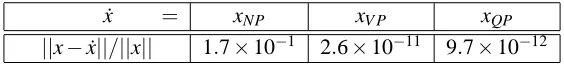
Example 4 This example illustrates that if one includes pivoting in the V method then the numerical

let C=

s2 10s 10s 200

, let the 4_×4 matrix K=

s2C 10sC 10sC 200C

. Now let x=

1/3 1/3

, w=

    0 x2 0 x1    ,

λ=0 let y=Kw.

Due to the structure of w (and since, in this example, a partial Cholesky factorization will move column 4 of K to the first column ofKe=PTKP) we again have each of xNP, xQPand xV Pwill cal-culate x exactly in exact arithmetic. In finite precision arithmetic the calcal-culated values will not be exact. For this example for small s the errors in both xV P and xQP are very small. For example if s=10−4we get the results in Table 4.

˙

x = xNP xV P xQP

||x₋x˙_||/_||x_|| 1.7_×10−1 2.6_×10−11 9.7_×10−12 Table 4: Errors_||x₋x˙_||/_||x_||for a 4_×4 matrices and various methods.

Note that even with pivoting the error in the normal equations approach is large. With the nor-mal equations approach the error in the calculated x includes a term proportional to cond2(K1). Even with pivoting cond2(K1)can be large enough so the accuracy of the normal equations ap-proach is poor.

7. Rank Selection

In using low rank approximation the choice of rank will affect the accuracy of the approximation. It may be impractical to repeat the computations for a variety of different ranks and it is useful to have techniques to facilitate determination of the accuracy of a variety of low rank approximations. We first consider the case that the true target values y∗corresponding to the testing data X∗are known. Then if n∗<n the accuracy of the prediction for y∗can be calculated efficiently for all low rank approximations with rank less than a specified value m.

To illustrate this we first consider the QR implementation, (12) and (13), of the subset of re-gressors method. For the(n+m)_×m matrix A in (8) let A=QR where Q is an(n+m)_×m matrix

with orthonormal columns and R is an m_×m upper triangular matrix and let x=R−1QTb, as in (12)

(where we omit the subscript Q on x to simplify our notation). Then by (13) the predicted values of

y∗are

b

y∗=K₁∗x

where K₁∗is the n∗_×m matrix defined in (3).

Now for some i, 1_≤i_≤m, consider the construction of a prediction for y∗using a rank i low rank approximation. LetA consist of the first i columns of A. It then follows from (9), (13) and thee

fact that the last m₋i rows of b andA are zero that the rank i prediction, which we calle ey∗, for y∗is given by solving

min

e

x || e

Axe₋b_||and letting

e y∗=K₁∗

where ex∈Ri and the 0 in (31) indicates a vector of m−i zeros. Since A=QR it follows that e

A=Q

e R

0

where the 0 here indicates m₋i rows of zeros. Therefore if c=(the first i elements

of QTb) it then follows (Golub and Van Loan, 1996, p. 239) that we can constructex using

e

x=Re−1c. (32)

We can use (32) to construct predictions for y∗ for every low rank approximation of rank less than or equal to m. To do this we let C be a m_×m upper triangular matrix whose ithcolumn consists of the first i elements of QTb and is zero otherwise. LetY be the ne ∗_×m matrix whose ith columns consists of the prediction for y∗using a rank i approximation. Then, for the reasons described in the last paragraph,

e

Y =K₁∗R−1C. (33)

If y∗is known (33) can be used to calculate, for example, the root mean square error of the prediction for y∗for all low rank approximations of rank less than or equal to m.

After the rank m low rank prediction for y∗is constructed, the above calculations require O(m3+ n∗m2)floating point operations. If n∗is less than n, this is less than the O(nm2)operations required to construct the initial rank m prediction. Although we will not present the details here similar efficiencies are possible when using the normal equations approach or the V method.

If the true value y∗for the test set are not known, one can use the subset of regressors approach to estimate the known y values in the training set (by replacing K₁∗ with K1 in (11), (13) or (16)).

Again one can calculate the accuracies in estimating y for every low rank approximation of rank less than a given rank m and this can be done relatively efficiently after the initial rank m low rank approximation is constructed. These accuracies will give some indication of the relative difference in using low rank approximations of different ranks.

Finally, we should note that our algorithms provide a limit on the largest rank that can be used. For example in SR-NP, SR-VP and SR-QP Algorithm 1 is used to determine the subset selection. Algorithm 1 returns a rank m where the factorization is stopped and m can be used as the maximum possible rank. For the SR-V and SR-Q algorithms a Cholesky factorization of K11 is required

in (7). If Matlab’s Cholesky routine chol is used for this factorization there is an option to stop the factorization when it is determined that K11 is not positive definite (numerically). The size

of the factor that successfully factors a positive definite portion of K11 sets a limit on the rank

that can be effectively used. Finally, SR-N and SR-NP require solving a system of Equations (5) involving the symmetric semidefinite systemλ2K11+K₁TK1. A good way to solve this system is to use Matlab’s chol, which again has an option that can be used to determine a limit on the rank that can be effectively used. As discussed in the next section if these rank limits are exceeded then the calculated answers are often dominated by computer arithmetic errors and are not accurate.

8. Practical Example

We illustrate our earlier remarks by using a training set of 180045 galaxies, each with five measured u, g, r, i, z broadband measurements. The training set consists of a 180045_×5 matrix

X of broadband measurements and the 180045_×1 vector y with the corresponding redshifts. The testing set will consist of a 20229×5 matrix X∗ of broadband measurements and the 20229×1 vector y∗of redshifts. This data is from the SDSS GOOD data set discussed in Way and Srivastava (2006).

To determine a good choice for a covariance function we calculated the root mean square (RMS) error for the prediction _by∗ for y∗ using the Matern (with parameter ν=3/2 and with parameter

ν=5/2), squared exponential, rational quadratic, quadratic and neural network covariance func-tions from Rasmussen and Williams (2006, Chap. 4). As mentioned earlier we selected the hyper-parameters for each covariance function using the Matlab routine minimize from Rasmussen and Williams (2006, pp. 112-116, 221). The covariance function which produced the smallest RMS error for the prediction of y∗was the neural network covariance function (Rasmussen and Williams, 2006, p. 91). For example, for low rank approximations of rank 500 with bootstrap resampling runs (described below) of size 100 the neural network median RMS error was .0204. The next small-est median RMS error was .0212 for the Matern covariance function withν=3/2 and the largest median RMS error was .0248 for the quadratic covariance function. Therefore in the experiments below we will use the neural network covariance function.

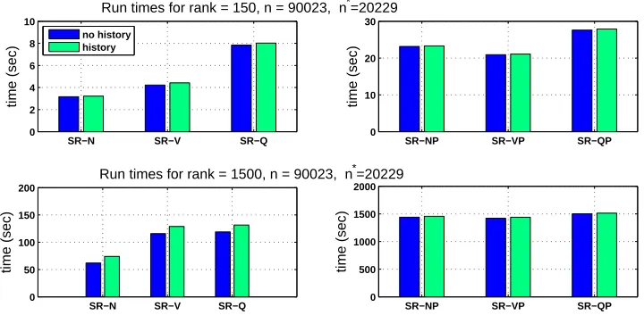
To compare, experimentally, the efficiency of our implementations of the subset of regressors method we choose a training set size of 90023 (consistent with the bootstrap resampling runs de-scribe below) and low rank approximations of rank m=150 and m=1500. On a computer with 2.2 GH Core Duo Intel processor we timed the SR-N, SR-V, SR-Q, SR-NP, SR-VP and SR-QP meth-ods. On all the calculations in this section that use Algorithm 1 we set the stopping tolerance tol to 0. We ran each of the methods with the additional calculations required to determine the “history” of the accuracy of all low rank approximations less than the specified rank (either 150 or 1500) and also without these extra calculations. The results are summarized in Figure 1.

SR−N SR−V SR−Q 0

2 4 6 8 10

Run times for rank = 150, n = 90023, n*=20229

time (sec)

no history history

SR−NP SR−VP SR−QP 0

10 20 30

time (sec)

SR−N SR−V SR−Q 0

50 100 150 200

Run times for rank = 1500, n = 90023, n*=20229

time (sec)

SR−NP SR−VP SR−QP 0

500 1000 1500 2000

time (sec)

As can be seen in Figure 1, without pivoting the normal equations approach is the fastest, the QR factorization the slowest and the V method in between. With pivoting all the methods take similar amounts of time (the V method is slightly faster). The reason that all the methods require about the same time when using pivoting is that the code for SR-N, SR-V and SR-Q is written so that the key calculations are done almost entirely with Matlab primitives whereas our implementation of the partial Cholesky factorization contains loops written in Matlab code. The Matlab primitives make use of BLAS-3 (Anderson et al., 1999) routines and will make effective use of cache memory. Therefore, even though the big-O operation counts are similar, the partial Cholesky factorization takes longer to run than SR-N, SR-V or SR-Q and the partial Cholesky factorization dominates the run times in the SR-NP, SR-VP and SR-QP code. We should add that the times for the partial Cholesky factorization would be reduced if a partial Cholesky factorization with pivoting could be implemented using BLAS-3 operations. We are not aware of such an implementation. Finally, we should note that the calculations required to determine the accuracy of all low-order approximations adds only a modest amount to the run times.

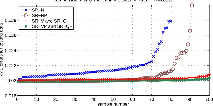
To determine the accuracy of the algorithms for different choices of the training set we carried out bootstrap resampling (Efron and Tibshirani, 1993). For each of 100 samples we randomly se-lected half or 90023 of the 180045 galaxies in the original training set and used this smaller training set to predict the redshift for the 20229 galaxies in the testing set. We considered such resam-pling with replacement as well as without replacement. For SR-N, SR-V and SR-Q we selected the indices in the active set randomly. Following this we selected the hyperparameters using the mini-mize routine in Rasmussen and Williams (2006, pp. 112-116, 221). For SR-NP, SR-VP and SR-QP the active set was determined by the partial Cholesky factorization with pivoting. To illustrate the variation in the calculated accuracies, after carrying out a bootstrap resampling run we sorted the 100 RMS errors in increasing order and plotted these errors versus the sample number. The results for low rank approximations of rank 1500, using resampling without replacement, are pictured in Figure 2.

Note that mathematically (in exact arithmetic) SR-N, SR-V and SR-Q will produce identical results; as will SR-NP, SR-VP and SR-QP. Therefore the differences illustrated in Figure 2 between SR-N and SR-V or SR-Q and the differences between SR-NP and SR-VP or SR-QP are due to com-puter arithmetic and, in particular, the numerical instabilities in using a normal equations approach to solve the least squares problem (9). Also note that although pivoting reduces the numerical instability in using the normal equations approach, still in SR-NP the instability is evident for ap-proximately half of the bootstrap resampling runs. Also we should remark that theyb∗predictions calculated using SR-V and SR-Q are essentially identical—they agree to at least seven significant digits in this example—as are the_by∗ predictions calculated using SR-VP and SR-QP. Finally we should note that for this example the methods that avoid normal equation and use pivoting—SR-VP and SR-QP—are a small amount better than their counterparts, SR-V and SR-Q, that do not use pivoting.

0 10 20 30 40 50 60 70 80 90 100 0.018

0.02 0.022 0.024 0.026 0.028

sample number

RMS errors for testing data

comparison of errors for rank = 1500, n = 90023, n*=20229

SR−N SR−NP

SR−V and SR−Q SR−VP and SR−QP

Figure 2: Bootstrap resampling: Comparison of RMS errors for implementations of the subset of regressors method.

We might also add that we tried other types of resampling. We obtained results similar to those illustrated in Figure 2 when using bootstrap resampling with replacement and also when we choose a number of galaxies in the sample size other than 90023.

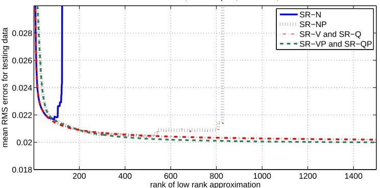
We can also illustrate the ability to efficiently calculate the accuracy of low rank approximations lower than a specified rank. For the same runs picture in Figure 2 we calculated the mean RMS error of the 100 samples for each rank less than 1500 for each of the six implementations of the subset of regressors method. This is pictured in Figure 3.

As one increases the rank of the low rank approximation the condition number of the matrix A in (9) will tend to increase. This will increase the computer arithmetic errors in the calculated results. The ranks where significant computer arithmetic errors arise are illustrated in Figure 3 by the jumps in the mean errors calculated for the SR-N and SR-NP methods. The ranks where this occurs and the magnitude of the jumps is dependent on the particular data chosen for a bootstrap resampling run and will vary for different bootstrap resampling runs. For the SR-N method the ranks where numerical difficulties were first substantial varied between a rank of 46 to a rank of 839. For the SR-NP method the ranks where numerical difficulties were first substantial varied between ranks of 325 and 1479. For the SR-V, SR-Q, SR-VP and SR-QP methods we did not encounter significant numerical difficulties with these runs and the graphs for these methods smoothly decrease.

200 400 600 800 1000 1200 1400 0.018

0.02 0.022 0.024 0.026 0.028

rank of low rank approximation

mean RMS errors for testing data

mean RMS errors vs. rank, 100 samples, n = 90023, n* = 20229

SR−N SR−NP

SR−V and SR−Q SR−VP and SR−QP

Figure 3: Mean RMS errors versus rank for implementations of the subset of regressors method.

As we mentioned earlier all of our algorithms may limit the rank so that the effective rank can be less than the desired rank. This did not occur on the above runs for SR-V, SR-Q, SR-VP or SR-QP but did occur for SR-N and SR-NP due to our use of the Cholesky factorization to solve the linear system (5). It is possible to solve the linear system in (5) using Gaussian elimination, rather than using a Cholesky factorization, for ranks up to 1500. However the Cholesky factorization in (5) will fail only if the matrixλ2K11+K₁TK1is very ill conditioned. In this case solving the system of equations in (5) by any method will be prone to large computer arithmetic errors. Indeed, for these runs, if we used Gaussian elimination to solve (5) for large ranks the errors became larger than when we limited the rank as we have described earlier. Also when the Cholesky factorization failed in the solution to (5) we tried perturbing K11a small amount following a suggestion in the code provided

with Rasmussen and Williams (2006). For our runs this did not improve the calculated results in a significant manner.

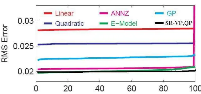
In Way and Srivastava (2006) there is a comparison of a variety of methods for predicting red-shift with data from the SLOAN digital sky survey. The methods compared in Way and Srivastava (2006) include linear regression, quadratic regression, artificial neural networks (label ANNz in Figure 4), E-model and Gaussian processes using a quadratic covariance function (labeled GP in Figure 4). In Figure 4 we have compared these methods with our predictions using the SR-VP and SR-QP implementations of the subset of regressors Gaussian processes method with a neural network covariance function. Other than the SR-VP and SR-QP predictions the results in Figure 4 are from Way and Srivastava (2006). As seen in Figure 4, in this example either SR-VP or SR-QP provides overall the best predictions. The E-model approach is also quite good.

Figure 4: Bootstrap resampling: comparison of RMS errors for six methods of predicting redshift.

the predictions were common for the SR-N and SR-NP algorithms. For some data sets, for exam-ple the SARCOS robot arm, computer arithmetic errors were not significant and all the algorithms worked well. Also we might note that although prediction using Gaussian processes was more ac-curate than alternatives approaches in some cases, in other cases the E-model or artificial neural network approaches provided better accuracy.

Finally, we should note that Matlab code which implements the SR-N, SR-NP, SR-V,SR-VP, SR-Q and SR-QP methods and can produce graphs such as those in Figures 2 and 3 is available at

http://dashlink.arc.nasa.gov/algorithm/stableGP. Our code makes use of the code from Rasmussen and Williams (2006, p. 221) and the syntax is modeled on that code. We should also note that Foster et al. (2008) and Cayco et al. (2006) discuss additional results related to redshift prediction.

9. Conclusions

An important conclusion of our results is that with the subset of regressors approach to Gaussian process calculations use of normal equations can be unstable and should, in some important prac-tical examples, be avoided. We expect that this principle is also applicable to other approaches to Gaussian process calculations. For example when using approximations based on sparse Gaussian processes with pseudo-inputs (Snelson and Ghahramani, 2006) which is called the FITC approx-imation in the framework of Quinonero-Candela and Rasmussen (2005) the predicted values are calculated using

b

y∗_FITC=K₁∗(λ2_K11+KT

1(Λ+I)−1K1)−1K1T(Λ+I)−1y.

where

Λ=diag(K₋K1K11−1K1T)/λ2.

Our results suggest that it may be more accurate to carry out these calculations using a QR

factor-ization of

DK1 λV₁₁T

where D= (Λ+I)−1/2_{rather than, for example, using a Cholesky factorization}

To summarize our results, we have presented different implementations of the subset of re-gressors method for solving, approximately, the Gaussian process equations for prediction. An implementation of the subset of regressors method which uses the normal equations is the fastest approach but also can have poor numerical stability and unacceptable large growth of computer arithmetic errors. An implementation using orthogonal factorization is somewhat slower but in principle has better numerical stability properties. A third approach, which we call the V method, is intermediate between these other two approaches in terms of accuracy and stability. We can use the partial Cholesky factorization to select the active set prior to implementation of any of the above methods. This also will tend to reduce the growth of computer arithmetic errors and can, in some cases, improve the accuracy of the predictions. All of these implementations require 0(nm2₎

operations where n is the number of data points in the training set and m is the size of the ac-tive set or the rank of the low rank approximation used. In this sense all these implementations are efficient and can be much faster than implementation of the full Gaussian process equations. Finally, we have illustrated these result with an important practical application—redshift predic-tion from broadband spectral measurements. Code implementing our algorithms is available at

http://dashlink.arc.nasa.gov/algorithm/stableGP.

Acknowledgments

We would like to acknowledge support for this project from the Woodward Fund, Department of Mathematics, San Jose State University.

M.J.W. acknowledges funding received from the NASA Applied Information Systems Research Program and from the NASA Ames Research Center Director’s Discretionary Fund. M.J.W also acknowledges Alex Szalay, Ani Thakar, Maria SanSebastien and especially Jim Gray for their help with the Sloan Digital Sky Survey.

A. N. Srivastava wishes to thank the NASA Aviation Safety Program, Integrated Vehicle Health Management Project for supporting this work.

Funding for the SDSS has been provided by the Alfred P. Sloan Foundation, the Participating Institutions, the National Aeronautics and Space Administration, the National Science Foundation, the U.S. Department of Energy, the Japanese Monbukagakusho, and the Max Planck Society. The SDSS Web site ishttp://www.sdss.org/.

The SDSS is managed by the Astrophysical Research Consortium for the Participating Institu-tions. The Participating Institutions are The University of Chicago, Fermilab, the Institute for Ad-vanced Study, the Japan Participation Group, The Johns Hopkins University, Los Alamos National Laboratory, the Max-Planck-Institute for Astronomy, the Max-Planck-Institute for Astrophysics, New Mexico State University, University of Pittsburgh, Princeton University, the United States Naval Observatory, and the University of Washington.

Appendix A. Numerical Stability of SR-VP

Here we explain why, even though there is a potential numerical instability in SR-V, as illustrated in Example 2, this difficulty cannot occur with the SR-VP method for small problems and is very unlikely to occur for larger problems from real world applications.

Let P be the n_×n permutation matrix determined by the partial Cholesky factorization with

pivoting applied to K, letKe=PTKP and letK1e be the first m columns ofK. In the SR-VP methode

we apply Equations (14)-(16) toK ande Ke1rather than K and K1.

We will begin by considering the special case whereλ=0 and later consider the more general case. In the case that λ=0 the least square problem (9), with K1 replaced byK1e since we are

incorporating pivoting, is equivalent to

min

x ||K1xe −y||.

and, by (15), we have

x=V₁₁−T(VTV)−1_VT_{y. (34)}

whereKe1=VV11T. There is a potential concern in using (34) since to construct x the linear system

of equations

(VTV)z=VTy

must be solved. Forming VTV squares the condition number of V which, potentially could lead to

the introduction of undesirable computer arithmetic errors. However we will argue that the matrix

B=VTV is diagonally equivalent to a matrix that is guaranteed to be well conditioned for small

problems and, in practice, is almost always well conditioned for larger problems. This will limit the growth of computer arithmetic errors. We should add that without pivoting one cannot prove such results, as is illustrated by Example 2.

Now V is formed by a partial Cholesky factorization with pivoting of the symmetric positive semidefinite matrix K. Since pivoting is included in the partial Cholesky factorization of the SPS matrix it follows, for each i=1, . . . ,m, that the ithdiagonal entry ofK1e is at least as large in magni-tude as any off diagonal entry in row i or column i ofK1e (Trefethen and Bau III, 1997, p. 176) and that the lower trapezoidal matrix V has the property that, for each i=1, . . . ,m, the ithdiagonal entry in V is at least as large in magnitude as any entry in column i (Higham, 2002, p. 202). Therefore we can write V as V=LD where D is an m_×m diagonal matrix and L is an n_×m lower trapezoidal

matrix with all entries one or less in magnitude and with ones on the diagonal. Indeed this matrix L is identical to the lower trapezoidal matrix produced if Gaussian elimination with complete pivoting is applied toK1e (Higham, 2002, p. 202). Also since the pivoting has already been applied in form-ingKe1Gaussian elimination with complete pivoting will not pivot any entries inKe1and this implies

that Gaussian with partial pivoting will not pivot any entries inKe1and will produce the same lower

trapezoidal factor L. Now it follows from Higham (2002, p. 148) that

cond(L)_≤√nm 2m−1

and therefore for n and m small, as in Example 2, L is well conditioned. More generally, according to Bj¨orck (1996, p. 73), if partial pivoting is used in the factorization ofKe1then L is usually well

Thus V is a diagonal rescaling of a matrix L that is well conditioned in practice. Now define

U=DV₁₁T. It then follows from (34) that

x=U−1(LTL)−1LTy. (35) Equation (35) is precisely the Peters-Wilkinson method (Peters and Wilkinson, 1970 and Bj¨orck, 1996, p. 73) to the least square problem (34). Since L is usually well conditioned then the calculation of(LTL)−1_LT_{y can be computed without substantial loss of accuracy and the calculation of x using}

(35) is more stable than using the normal equation solution to (34) (Bj¨orck, 1996, p. 73).

The SR-VP method uses (34) rather that (35). However, since V is a diagonal rescaling of L and

U is a diagonal rescaling of V₁₁T the SR-VP method will also have good numerical stability properties in practice. To demonstrate this we can write V=LD1D2where the entries of the diagonal matrix D1

are between 1 and 2 and where entries in D2are exact powers of 2. Since L will be well conditioned

in practice then so is W=LD1(since cond(LD1)≤cond(L)cond(D1)≤2 cond(L)). Now, by (34),

we have

x= (D2V11)−T(WTW)−1WTy. (36)

Since W is well conditioned in practice it follows, for the same reasons that (35) has good numerical stability, that (36) will have good numerical stability properties.

To finish the analysis of numerical stability of the SR-VP method in the case thatλ=0 note that since D2 has entries that are exact powers of 2, it follows by the discussion in Higham (2002,

p. 200) and Forsythe and Moler (1967, 37-39), for any computer using base 2 computer arithmetic, that the x calculated by (36) will be precisely the same, even in floating point arithmetic (as long as there is no overflow or underflow), as the x calculated by (34). Therefore we may conclude that in practice x calculated when using the SR-VP method will have good numerical stability properties and the SR-VP method will usually have smaller computer arithmetic errors than will the SR-N or SR-NP methods.

To consider the case thatλ₆=0 we note that in this case the condition number of B= (λ2_I+VT_V)

will be important in solving

(λ2_I+VT_V)z=VT_y.

However we have

Theorem 3 For anyλ_≥0, cond(λ2_I+VT_V)≤cond(VT_V).

Proof If VTV has eigenvaluesα1≥α2≥. . .≥αm≥0 then the eigenvalues of (λ2I+VTV) are (λ2₊α

i), i=1, . . . ,m. Therefore cond(VTV) =α1/αmand cond(λ2I+VTV) = (α1+λ2)/(αm+ λ2_{). However it follows easily that}α_1/α

m≥(α1+λ2)/(αm+λ2).

Since cond(λ2_I+VT_V)≤cond(VT_{V)we expect that solving(λ}2_I+VT_V)z=VT_{y withλ6=0}