Partial Label Learning via Label Enhancement

(1)

The Thirty-Third AAAI Conference on Artificial Intelligence (AAAI-19)

Partial Label Learning via Label Enhancement

Ning Xu, Jiaqi Lv, Xin Geng

∗

MOE Key Laboratory of Computer Network and Information Integration, China School of Computer Science and Engineering, Southeast University, Nanjing 210096, China

{xning, lvjiaqi, xgeng}@seu.edu.cn

Abstract

Partial label learning aims to learn from training examples each associated with a set of candidate labels, among which only one label is valid for the training example. The com-mon strategy to induce predictive model is trying to disam-biguate the candidate label set, such as disambiguation by identifying the ground-truth label iteratively or disambigua-tion by treating each candidate label equally. Nonetheless,

these strategies ignore considering the generalizedlabel

dis-tributioncorresponding to each instance since the

general-ized label distribution is not explicitly available in the training set. In this paper, a new partial label learning strategy named

PL-LEis proposed to learn from partial label examples via

label enhancement. Specifically, the generalized label distri-butions are recovered by leveraging the topological informa-tion of the feature space. After that, a multi-class predictive model is learned by fitting a regularized multi-output regres-sor with the generalized label distributions. Extensive

exper-iments show that PL-LEperforms favorably against

state-of-the-art partial label learning approaches.

Introduction

Partial label (PL) learning deals with the problem where each training example is associated with a set of candi-date labels, among which only one label is valid (Cour, Sapp, and Taskar 2011; Chen et al. 2014; Yu and Zhang 2017). In recent years, partial label learning techniques have been found useful in solving many real-world scenarios such as web mining (Jie and Orabona 2010), multimedia content analysis (Zeng et al. 2013; Chen, Patel, and Chel-lappa in press), ecoinformatics (Liu and Dietterich 2012; Tang and Zhang 2017), etc.

Formally speaking, let X = _Rq _{be the} _q_-dimensional instance space and Y = {y1, y2, y3, ..., yc} be the label space with c class labels. Given the partial label training setD = {(xi, Si)|1 ≤ i ≤ n}, the task of partial label learning is to induce a multi-class classifier f : X 7→ Y

fromD. Here,xi∈ X is aq-dimensional feature vector and Si ⊆ Y is the associated candidate label set. Partial label learning takes the key assumption that the ground-truth la-belyi corresponding toxiresides in its candidate label set

∗

Corresponding author

Copyright c2019, Association for the Advancement of Artificial

Siand therefore cannot be directly accessed by the learning algorithm.

Intuitively, the basic strategy for handling partial label learning problem is disambiguation, i.e., trying to identify the ground-truth label from the candidate label set associ-ated with each training example, where existing strategies include disambiguation by identification or disambiguation by averaging. For identification-based disambiguation, the ground-truth label is regarded as latent variable and iden-tified through iterative refining procedure such as EM (Jin and Ghahramani 2003; Nguyen and Caruana 2008; Liu and Dietterich 2012; Chen et al. 2014; Yu and Zhang 2017). For averaging-based disambiguation, all the candidate labels are treated equally and the prediction is made by averag-ing their modelaverag-ing outputs (H¨ullermeier and Beraverag-inger 2006; Cour, Sapp, and Taskar 2011; Zhang and Yu 2015).

In order to handle partial label learning problem, we can explicitly assign adescription degreeto each label instead of disambiguation. This is similar tolabel distribution learning (LDL) (Geng 2016). In LDL, the description degreesdyj

x of

all the labels constitute a real-valued vector calledlabel dis-tribution. Heredyj

x ∈ [0,1]andP_ydyx = 1. Note that the

normalized labeling confidence vector in the feature-ware PL approach (Zhang, Zhou, and Liu 2016) can be viewed as label distribution. In order to accommodate more flexibil-ity on PL data sets, the description degree is generalized in this paper: 1)dyj

x ∈(0,1),∀yj ∈Sidenotes the label rele-vance over each candidate label. 2)dyj

x ∈(−1,0),∀yj ∈/ Si

denotes the label irrelevance over each non-candidate label. Then, the generalized description degrees (GDD) of all the labels constitute the generalized label distribution (GLD).

GDDs in partial label learning are essentially relative in mainly two aspects:

• The relevance among candidate labels is different rather than exactly equal. For example, in Figure 1(a), candidate painting style can be freely provided by web users, while the relevance of each style is different.

• The irrelevance of each non-candidate label may be very different. For example, in Figure 1(b), for a car, the label airplane is more irrelevant than the label tank.

(2)

Annotation from user A:Monet style

Annotation from user B: Picasso style

Annotation from user C: Van Gogh style

(a) Online object annotation (b) Target

Figure 1: Two examples about the generalized description degrees in partial label learning.

(Xu, Tao, and Geng 2018). Accordingly, a novel partial label learning algorithm named PL-LE, i.e.,Partial Label learning via Label Enhancement, is proposed in this paper. PL-LEcan recover flexible GLDs via leveraging the topological infor-mation of the feature space. After that, a multi-class predic-tive model is learned by fitting a regularized multi-output regressor with the recovered GLDs.

The rest of this paper is organized as follows. Firstly, re-lated works on partial label learning are briefly reviewed. Secondly, technical details of the proposed approach are in-troduced. Thirdly, the results of the comparative experiments are reported. Finally, we conclude this paper.

Related Work

As shown in Section 1, supervision information conveyed by PL training examples is implicit as the ground-truth label is hidden within the candidate label set. Therefore, partial label learning can be regarded as a weak supervi-sionlearning framework with implicit labeling information. Generally, partial label learning is related to several well-established weakly-supervised learning frameworks such as semi-supervised learning, multi-instance learning and multi-label learning. Nevertheless, the type of weak supervi-sion information handled by partial label learning is different to those counterpart frameworks.

In semi-supervised learning (Zhu and Goldberg 2009), the task is to learn a classifierf :X 7→ Yfrom both labeled and unlabeled examples. For unlabeled data the ground-truth label assumes the entire label space, while for PL data the ground-truth label is confined within its candidate label set. In multi-instance learning (Amores 2013), the task is to learn a classifierf : 2X 7→ Y from examples each repre-sented as a labeled bag of instances, where a single label is assigned to a set of instances for multi-instance example while a set of labels are assigned to a single instance for PL example. Inmulti-label learning(Zhang and Zhou 2014; Hou, Geng, and Zhang 2016), the task is to learn a classifier f : X 7→ 2Y from training examples each associated with multiple labels, where the associated labels are all valid ones for multi-label example while the associated labels are only candidate ones for PL example.

Most existing algorithms aim to fulfill the learning task by fitting widely-used learning techniques to partial label data. For maximum likelihood techniques, the likelihood of observing each PL training example is defined over its

candidate label set instead of the unknown ground-truth la-bel (Jin and Ghahramani 2003; Liu and Dietterich 2012). K-nearest neighbor techniques determine class label of un-seen instance via voting among the candidate labels of its neighboring examples (H¨ullermeier and Beringer 2006; Zhang and Yu 2015). For maximum margin techniques, the classification margins over the PL training examples are de-fined by discriminating modeling outputs from candidate la-bels and non-candidate lala-bels (Nguyen and Caruana 2008; Yu and Zhang 2017). For boosting techniques, the weight over each PL training example and the confidence over the candidate labels are updated in each boosting round (Tang and Zhang 2017).

Other than the above-mentioned works, there are a few works which work by fitting PL data to existing learning techniques. The CLPL approach (Cour, Sapp, and Taskar 2011) maps a d-dimensional instance in X into ad×q -dimensional feature vector for each class label inY. For each PL training example(xi, Si), one positive example is gen-erated by averaging mapped feature vectors w.r.t. candidate labels inSiandq− |Si|negative examples are generated by taking the mapped feature vector w.r.t. each non-candidate label in Y \Si. The PL-ECOC approach (Zhang, Yu, and Tang 2017) transforms each instance into a binary example via leveraging ECOC coding matrix (Dietterich and Bakiri 1995; Zhou 2012). For each PL training example(xi, Si), it is regarded as a positive or negative example if its candidate label setSi entirely falls into the column dichotomy of the coding matrix.

In the next section, a novel partial label learning ap-proach will be introduced. Different from existing partial la-bel learning approaches, the generalized lala-bel distributions are recovered and utilized to facilitate the learning proce-dure. To our best knowledge, it is the first attempt to propose GLD to solve PL problem via label enhancement.

The Proposed Approach

As shown in Section 1, the task of partial label learning is to induce a multi-class classifierf :X 7→ Y from the par-tial label training setD = {(xi, Si)|1 ≤ i ≤n}. Specifi-cally, for each PL training example(xi, Si), the logical label vector li = (ly1

xi, lyxi2, ..., lxiyc)> ∈ {−1,1}c is used to

rep-resent whether each label yj is among the candidate label set. In the proposed approach, GLD is denoted by the vector di= (dyx1i, d

y2 xi, ..., d

yc

xi)

>_.

In the next subsections, the two stages of PL-LE, i.e., gen-eralized label distribution recovery and predictive model in-duction, will be scrutinized respectively.

Generalized Label Distribution Recovery

Given a PL training set D, we construct the feature ma-trix X = [x1,x2, ...,xn] and the logical label matrix L = [l1,l2, ...,ln]. To recover the reasonable GLD matrix D= [d1,d2, ...,dn], we consider the model

di =W>ϕ(xi) +s= ˆW φi, (1)

where W = [w1_{, ...,}_wc_] _{is a weight matrix and} _s ₌

(3)

transforma-tion ofxto a higher dimensional feature space. For conve-nient describing, we setWˆ = [W>_,_s_]_and_φ

i = [ϕ(xi); 1]. Accordingly, the goal of our method is to determine the best parameterWˆ ∗that can generate a reasonable GLDdigiven the instancexi. Then, the optimization problem becomes

min

ˆ

W

L( ˆW) +λR( ˆW), (2)

whereLis a loss function,Ris the function to mine hidden GDDs, andλis the parameter trading off the two terms. Note that GLD recovery is essentially a pre-processing applied to the training set, which is different from standard supervised learning. Therefore, we does not need to consider the over-fitting problem. Since the labeling information in GLD is inherited from the initial logical labels, we choose the least squares (LS) loss function as

L( ˆW) =

n X

i=1

kW φiˆ −lik2

= tr[( ˆWΦ−L)>( ˆWΦ−L)],

(3)

whereΦ= [φ1, ...,φn].

By leveraging the topological information of the feature space, hidden GDDs can be mined from the training exam-ples. Therefore, we specify then×nlocal similarity matrix Awhose elements are calculated as follows.

• Step 1. We put an edge betweenxiandxjifxiis among K-nearest neighbors of xj or xj is among K-nearest neighbors ofxi.

• Step 2. Ifxiandxjare connected,aijis specified as

aij = exp −

kxi−xjk

2

2 !

. (4)

Otherwise,aijis set to 0.

According to the smoothness assumption (Zhu, Lafferty, and Rosenfeld 2005), if xi andxj have a high degree of similarity, as measured byaij, thendianddjshould be near to one another. This intuition leads to the following function which we wish to minimize:

R( ˆW) =X

i,j

aijkdi−djk2

= tr(DGD>)

= tr( ˆWΦGΦ>Wˆ >),

(5)

whereG = ˆA−A is the graph Laplacian andAˆ is the

diagonal matrix whose elements areˆaii= n P

j=1

aij.

Formulating the GLD recovery problem into an optimiza-tion framework over Eq. (3) and Eq. (5) yields the target function ofWˆ

T( ˆW) = tr[( ˆWΦ−L)>( ˆWΦ−L)]

+λtr( ˆWΦGΦ>Wˆ >). (6)

Besides, we add a constraint to ensure that the GDD in re-covered GLD possesses the same sign with the logical label and takes value with reasonable magnitude:

∀1≤i≤n,1≤j≤c,0< dyj

xil

yj

xi<1. (7)

Note that Eq. (6) can be rewritten as:

T( ˆw) =

c X

j=1

ˆ

wj(ΦΦ>+ 2λΦGΦ>) ˆwj>

−2 ˆwjΦlj+ljlj>,

(8)

wherewˆj _{is the}_j_{-th row of the parameter matrix}_Wˆ _and_lj is the j-th row of the logical label matrixL. Accordingly, for the parameter matrixWˆ , itsj-th rowwˆj can be deter-mined by solving the following constrained quadratic pro-gramming process:

min

ˆ

wj wˆ

j₍_ΦΦ>_{+ 2}_λ_Φ_G_Φ>_{) ˆ}_wj>₋_{2 ˆ}_wj_Φ_lj

s.t. 0< dyj

xil

yj

xi<1,∀1≤i≤n.

(9)

When the best parameterWˆ ∗is determined, the generalized label distributiondican be generated through Eq. (1).

Predictive Model Induction

Given the recovereddiofxi, the original PL training set can be transformed intoE = {(xi,di)|1 ≤ i ≤ n}. Asdi for each training example(xi,di)is numerical, it is natural to induce the predictive model by employing multi-output re-gression techniques. Similar to the MSVR, we generalize a regressor to solve the multi-dimensional case. In addition, our regressor not only concerns the distance between the predicted and the real values, but also the sign consistency of them. It leads to the minimization of

Ω(Θ,b) = 1 2

c X

j=1

kθjk2₊_C

1 n X

i=1

Ω1i+C2 n X

i=1

Ω2i, (10)

whereΘ = [θ1_{, ...,}_θc_]_,_b_{= [}_b1_{, ..., b}c_]_,_Ω

1andΩ2are the regression loss and the sign loss, respectively.

As shown in Eq. 10, the first term ofΩ(Θ,b)controls the complexity of the induced model. In addition, the second term ofΩ(Θ,b)is defined to consider all dimensions into a unique restriction and yield a single support vector for all dimensions:

Ω1i=

₀ _r

i< ε r2

i −2riε+ε2 ri≥ε,

(11)

whereri=keik= p

e>_i ei,ei =di−ϕ(xi)>Θ−b. This will create an insensitive zone determined byεaround the estimate, i.e., the loss ofrless thanεwill be ignored. The third term is used to make the signs of the predictive output and the logical label same as much as possible:

Ω2i=− c X

j=1

(4)

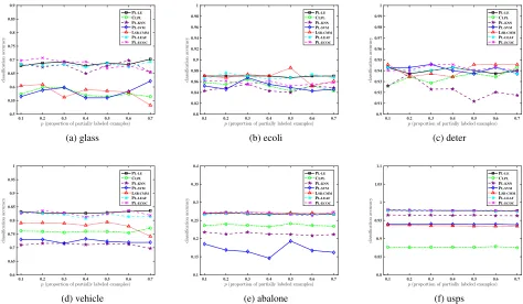
0.1 0.2 0.3 0.4 0.5 0.6 0.7 p(proportion of partially labeled examples)

0.5 0.55 0.6 0.65 0.7 0.75 0.8 0.85 0.9 cl as si fi ca ti on ac cu ra cy PL-LE CLPL PL-KNN PL-SVM LSB-CMM PL-LEAF PL-ECOC (a) glass

0.8 0.82 0.84 0.86 0.88 0.9 0.92 0.94 0.96 0.98 1 cl as si fi ca ti on ac cu ra cy PL-LE CLPL PL-KNN PL-SVM LSB-CMM PL-LEAF PL-ECOC (b) ecoli

0.9 0.91 0.92 0.93 0.94 0.95 0.96 0.97 0.98 0.99 1 cl as si fi ca ti on ac cu ra cy PL-LE CLPL PL-KNN PL-SVM LSB-CMM PL-LEAF PL-ECOC (c) deter

0.6 0.65 0.7 0.75 0.8 0.85 0.9 0.95 1 cl as si fi ca ti on ac cu ra cy PL-LE CLPL PL-KNN PL-SVM LSB-CMM PL-LEAF PL-ECOC (d) vehicle

0.1 0.2 0.3 0.4 0.5 0.6 0.7

p(proportion of partially labeled examples)

0.1 0.15 0.2 0.25 0.3 0.35 0.4 cl as si fi ca ti on ac cu ra cy PL-LE CLPL PL-KNN PL-SVM LSB-CMM PL-LEAF PL-ECOC (e) abalone

0.8 0.85 0.9 0.95 1 1.05 1.1 cl as si fi ca ti on ac cu ra cy PL-LE CLPL PL-KNN PL-SVM LSB-CMM PL-LEAF PL-ECOC (f) usps

Figure 2: Classification accuracy of each comparing algorithm changes asp(proportion of partially labeled examples) increases from 0.1 to 0.7 (with one false positive candidate label[r= 1]).

The meaning of Eq. (12) is that if the signs of the predictive output and the logical label are different, there will be some positive loss, otherwise the loss will be negative.

To minimizeΩ(Θ,b), we use an iterative quasi-Newton method called Iterative Re-Weighted Least Square (IRWLS) (P´erez-Cruz et al. 2000). Firstly,Ω1(Θ,b)is approximated by its first order Taylor expansion at the solution of the cur-rentk-th iteration, denoted byΘ(k)_and_b(k)_:

Ω0₁_i=Ω(₁k_i)+dΩ1 dr

_r(k)

i

(e(_ik))>

r(_ik)

ei−e(_ik), (13)

wheree(_ik)andr_i(k)are calculated fromΘ(k)andb(k). Then a quadratic approximation is further constructed as

Ω00₁_i=Ω(₁k_i)+dΩ1 dr

_r(k)

i

r2 i −(r

(k) i )2

2r(_ik)

=1 2air

2 i +τ,

(14)

where

ai =

1

r(_ik) dΩ1

dr _r(k)

i

=  



0 r_i(k)< ε

2r(_ik)−ε r(_ik) r

(k) i ≥ε,

(15)

Table 1: Characteristics of the controlled UCI data sets.

Data Set #Examples #Features # Labels

glass 214 9 6

ecoli 336 7 8

deter 358 23 6

vehicle 846 18 4

abalone 4,177 7 29

usps 9,298 256 10

Configurations

(I) r= 1,p∈ {0.1,0.2, . . . ,0.7}

(II) r= 2,p∈ {0.1,0.2, . . . ,0.7}

(III)r= 3,p∈ {0.1,0.2, . . . ,0.7}

(IV)p= 1,r= 1,∈ {0.1,0.2, . . . ,0.7}

andτis a constant term that does not depend on eitherΘ(k) orb(k)_{. Combining Eq. (10), (12) and (14), we can get}

Ω00(Θ,b) = 1 2

c X

j=1

kθjk2₊1

2C1

n X

i=1

air2i

−C2

n X i=1 c X j=1

lj_i(ϕ(xi)>θj+bj) +τ.

(16)

(5)

0.1 0.2 0.3 0.4 0.5 0.6 0.7

ǫ(co-occurring probability of the coupling label)

0.3 0.4 0.5 0.6 0.7 0.8 0.9 cl as si fi ca ti on ac cu ra cy PL-LE CLPL PL-KNN PL-SVM LSB-CMM PL-LEAF PL-ECOC (a) glass

0.1 0.2 0.3 0.4 0.5 0.6 0.7

0.7 0.75 0.8 0.85 0.9 0.95 1 cl as si fi ca ti on ac cu ra cy PL-LE CLPL PL-KNN PL-SVM LSB-CMM PL-LEAF PL-ECOC (b) ecoli

0.1 0.2 0.3 0.4 0.5 0.6 0.7

0.8 0.85 0.9 0.95 1 1.05 1.1 cl as si fi ca ti on ac cu ra cy PL-LE CLPL PL-KNN PL-SVM LSB-CMM PL-LEAF PL-ECOC (c) deter

0.1 0.2 0.3 0.4 0.5 0.6 0.7

0.6 0.65 0.7 0.75 0.8 0.85 0.9 0.95 1 cl as si fi ca ti on ac cu ra cy PL-LE CLPL PL-KNN PL-SVM LSB-CMM PL-LEAF PL-ECOC (d) vehicle

0.1 0.2 0.3 0.4 0.5 0.6 0.7

0.1 0.15 0.2 0.25 0.3 0.35 0.4 cl as si fi ca ti on ac cu ra cy PL-LE CLPL PL-KNN PL-SVM LSB-CMM PL-LEAF PL-ECOC (e) abalone

0.1 0.2 0.3 0.4 0.5 0.6 0.7

0.8 0.85 0.9 0.95 1 1.05 1.1 cl as si fi ca ti on ac cu ra cy PL-LE CLPL PL-KNN PL-SVM LSB-CMM PL-LEAF PL-ECOC (f) usps

Figure 3: Classification accuracy of each comparing algorithm changes as(co-occurring probability of the coupling label) increases from 0.1 to 0.7 (with 100% partially labeled examples [p= 1] and one false positive candidate label [r= 1]).

1, . . . , c:

C1Φ>FΦ+I C1Φ>a

C1a>Φ C11>a

θj

bj

=

C1Φ>F dj₊_C2_Φ>_lj

C1a>dj+C21>lj

,

(17) whereΦ = [ϕ(x1), ..., ϕ(xn)]>,a = [a1, ..., an]>,Fik = aiδki (δ

k

i is the Kronecker’s delta function), and l j ₌

[lj₁, . . . , lj

n]>. Then, the direction of the optimal solution of Eq. (17) is used as the descending direction for the opti-mization ofΩ(Θ,b), and the solution for the next iteration (Θ(k+1)_and_b(k+1)_{) is obtained via a line search algorithm} along this direction.

According to the representor’s theorem (Smola 1999), un-der fairly general conditions, a learning problem can be ex-pressed as a linear combination of the training examples in the feature space, i.e.θj ₌P

iηjϕ(xi). If we replace this expression into Eq. (9) and Eq. (17), it will generate the in-ner product< ϕ(xi), ϕ(xj)>, and then the kernel trick can be applied.

LetΘ∗andb∗be the resulting model after the whole it-erative optimization process, PL-LEmakes prediction on the class label of unseen instancexas follows:

f(x) = arg max

yj∈Y

ϕ(x)>θ∗j+b∗j (18)

Experiments

Methodology

The performance of PL-LE is compared against six state-of-the-art partial label learning approaches, each configured with parameters suggested in respective literature:

• CLPL (Cour, Sapp, and Taskar 2011) which transforms partial label learning problem into binary learning prob-lem via feature mapping with convex loss optimization [suggested configuration: SVM with squared hinge loss].

• PL-KNN (H¨ullermeier and Beringer 2006) which adopts K-nearest neighbor technique to learn from PL data via weighted voting [suggested configuration:k= 10].

• PL-SVM(Nguyen and Caruana 2008) which adopts max-imum margin technique to learn from PL data vial2 regu-larization [suggested configuration: reguregu-larization param-eter pool with{10−3_{, . . . ,}₁₀3_}_].

• LSB-CMM(Liu and Dietterich 2012) which adopts maxi-mum likelihood to learn from PL data via mixture models [suggested configuration:5qmixture components].

• PL-LEAF (Zhang, Zhou, and Liu 2016) which adopts a two-stage approach to learn from partial label examples based on feature-aware disambiguation. [suggested con-figuration:K= 10,C1= 10,C2= 1].

(6)

prob-Table 2: Win/tie/loss counts (pairwiset-test at 0.05 significance level) on the classification performance of PL-LEagainst each comparing approach.

PL-LEagainst

CLPL PL-KNN PL-SVM LSB-CMM PL-LEAF PL-ECOC

varyingp[r=1] 26/16/0 20/20/0 23/19/0 12/30/0 0/42/0 0/42/0

varyingp[r=2] 27/15/0 26/16/0 24/18/0 12/30/0 0/42/0 1/41/0

varyingp[r=3] 27/15/0 25/17/0 27/15/0 15/27/0 2/40/0 1/41/0

varying[p, r=1] 25/17/0 28/14/0 28/14/0 24/18/0 8/34/0 6/36/0

In Total 105/63/0 101/67/0 102/66/0 63/105/0 10/158/0 8/160/0

Table 3: Characteristic of the real-world partial label data sets.

Data Set #Examples #Features #Class Labels avg. #CLs Task Domain FG-NET 1,002 262 78 7.48 facial age estimation(Panis and Lanitis 2015)

Lost 1,122 108 16 2.23 automatic face naming(Cour, Sapp, and Taskar 2011)

MSRCv2 1,758 48 23 3.16 object classification(Liu and Dietterich 2012)

BirdSong 4,998 38 13 2.18 bird song classification(Briggs, Fern, and Raich 2012)

Soccer Player 17,472 279 171 2.09 automatic face naming(Zeng et al. 2013)

Yahoo! News 22,991 163 219 1.91 automatic face naming(Guillaumin, Verbeek, and Schmid 2010)

lem via ECOC coding matrix [suggested configuration: codeword lengthL=d10 log₂(q)e].

For PL-LE, the parameterλis set to 0.01 and the number of neighborsKis set to 20. The parametersC1andC2 are set to 1 and 1, respectively. The kernel function in PL-LEis Gaussian kernel.

Controlled UCI Data Sets

Table 1 summarizes the characteristics of six controlled UCI data sets (Bache and Lichman 2013). Concretely, follow-ing the widely-used controllfollow-ing protocol, an artificial par-tial label data set is derived from one multi-class UCI data set by configuring three controlling parameters p, r and (Cour, Sapp, and Taskar 2011; Liu and Dietterich 2012; Chen et al. 2014; Zhang, Yu, and Tang 2017). Here,p con-trols the proportion of examples which are partially labeled (i.e.|Si|>1),rcontrols the number of false positive labels in the candidate label set (i.e.|Si|=r+1), andcontrols the co-occurring probability between one extra candidate label and the ground-truth label. As shown in Table 1, a total of 28 (4×7) parameter configurations are considered for each controlled UCI data set.

Figure 2 illustrates the classification accuracy of each comparing algorithm as p increases from 0.1 to 0.7 with step-size 0.1 (r= 1). Along with the ground-truth label, one class label inYwill be randomly picked up to constitute the candidate label set. Due to page limit, figures for the cases ofr= 2andr= 3are not illustrated here while similar re-sults to Figure 2 can be observed as well. Figure 3 illustrates the classification accuracy of each comparing algorithm as increases from 0.1 to 0.7 with step-size 0.1 (p= 1, r = 1). Given any labely∈ Y, one extra labely0 ∈ Yis designated as the coupling label which co-occurs withy in the candi-date label set with probability. Otherwise, any other class label would be randomly chosen to co-occur withy.

As illustrated in Figures 2 and 3, the performance of PL

-LE is highly competitive to other comparing algorithms in most cases. Furthermore, pairwiset-test at 0.05 significance level is conducted based on the results of ten-fold cross-validation. Table 2 reports the win/tie/loss counts between PL-LEand each comparing approach. Specifically, out of the 168 statistical tests (28 configurations x 6 UCI data sets), it is shown that:

• Across all the controlling parameter configurations and controlled UCI data sets, none of the comparing algo-rithms have outperformed PL-LEsignificantly.

• Comparing to averaging-based disambiguation ap-proaches (in total), PL-LEachieves superior performance against CLPL and PL-KNN in 62.5% cases (105 out of 168) and 60.1% cases (101 out of 168) respectively.

• Comparing to identification-based disambiguation ap-proaches (in total), PL-LEachieves superior performance against PL-SVM and LSB-CMMin 60.7% cases (102 out of 168) and 37.5% cases (63 out of 168) respectively.

• PL-LE achieves comparable performance against PL

-LEAFand PL-ECOCin 94.0% cases (158 out of 168) and 95.2% cases (160 out of 168) respectively. In addition, PL-LE achieves superior performance against PL-LEAF

and PL-ECOC in 6.0% cases (10 out of 168) and 4.8% cases (9 out of 168) respectively.

Real-World Data Sets

Table 3 summarizes the characteristics of real-world partial label data sets, which are collected from several application domains includingFG-NET(Panis and Lanitis 2015) for fa-cial age estimation,Lost (Cour, Sapp, and Taskar 2011),

Soccer Player(Zeng et al. 2013) and Yahoo!News

(7)

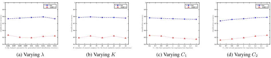
0.006 0.007 0.008 0.009 0.01 0.011 0.012 0.013 0.014

λ(the balance parameter for generalized label distribution recovery) 0.4

0.5 0.6 0.7 0.8 0.9 1

cl

as

si

fi

ca

ti

on

ac

cu

ra

cy

lost MSRCv2

(a) Varyingλ

16 17 18 19 20 21 22 23 24

K(number of nearest neighors for the local similarity matrix construction)

0.4 0.5 0.6 0.7 0.8 0.9 1

cl

as

si

fi

ca

ti

on

ac

cu

ra

cy

lost MSRCv2

(b) VaryingK

0.6 0.7 0.8 0.9 1 1.1 1.2 1.3 1.4

C1(thefirst parameter for regression loss function)

0.4 0.5 0.6 0.7 0.8 0.9 1

cl

as

si

fi

ca

ti

on

ac

cu

ra

cy

lost MSRCv2

(c) VaryingC1

0.6 0.7 0.8 0.9 1 1.1 1.2 1.3 1.4

C2(the second parameter for regression loss function) 0.4

0.5 0.6 0.7 0.8 0.9 1

cl

as

si

fi

ca

ti

on

ac

cu

ra

cy

lost MSRCv2

(d) VaryingC2

Figure 4: Parameter sensitivity analysis for PL-LEon theLostandMSRCv2data sets. (a) Classification accuracy of PL-LE

changes asλincreases from 0.006 to 0.014 with step-size 0.002(K = 20, C1 = 1, C2 = 1); (b) Classification accuracy of PL-LEchanges asKincreases from 16 to 24 with step-size 2(λ= 0.01, C1= 1, C2= 1); (c) Classification accuracy of PL-LE changes asC1increases from 0.6 to 1.4 with step-size 0.2(λ= 0.01, K = 20, C2= 1); (d) Classification accuracy of PL-LE changes asC2increases from 0.6 to 1.4 with step-size 0.2(λ= 0.01, K = 20, C1= 1).

Table 4: Classification accuracy (mean±std) of each comparing algorithm on the real-world partial label data sets. In addition,

•/◦ indicates whether is statistically superior/inferior to the comparing algorithm on each data set (pairwise t-test at 0.05 significance level).

FG-NET Lost MSRCv2 BirdSong Soccer Player Yahoo! News

PL-LE 0.082±0.023 0.773±0.043 0.499±0.037 0.730±0.013 0.536±0.020 0.653±0.006

CLPL 0.063±0.027 0.742±0.038 0.413±0.041• 0.632±0.019• 0.368±0.010• 0.462±0.009•

PL-KNN 0.038±0.025• 0.424±0.036• 0.448±0.037• 0.614±0.021• 0.497±0.015• 0.457±0.004•

PL-SVM 0.063±0.029 0.729±0.042• 0.461±0.046 0.660±0.037• 0.464±0.011• 0.629±0.010•

LSB-CMM 0.059±0.025 0.693±0.035• 0.473±0.037 0.672±0.056• 0.498±0.017• 0.645±0.005•

PL-LEAF 0.076±0.037 0.717±0.059• 0.498±0.035 0.723±0.013 0.532±0.017 0.641±0.006•

PL-ECOC 0.040±0.018• 0.653±0.053• 0.440±0.039• 0.731±0.013 0.494±0.015• 0.610±0.009•

2012) for object classification, and BirdSong (Briggs, Fern, and Raich 2012) for bird song classification. The av-erage number of candidate labels (avg. #CLs) for each real-world partial label data set is also recorded in Table 3.

Table 4 reports the mean classification accuracy as well as standard deviation of each comparing algorithm. Pairwise t-test at 0.05 significance level is conducted based on the ten-fold cross-validation, where the test outcomes between PL-LEand the comparing approaches are also recorded.

As shown in Table 4, it is impressive to observe that:

• On all data sets, PL-LE achieves superior or at least comparable performance against all the comparing ap-proaches.

• On all data sets, PL-LE significantly outperforms PL

-KNN.

• PL-LE significantly outperforms PL-ECOC onFG-NET,

Lost,MSRCv2,Soccer PlayerandYahoo!News.

• PL-LEachieves superior performance against all the com-paring approaches except PL-LEAFon the two large-scale data sets (Soccer PlayerandYahoo!News) . Note that the proposed method performs better on larger datasets. It is because that label enhancement can better re-cover the hidden GLD in lager datasets.

Sensitivity Analysis

In this subsection, performance sensitivity of the proposed PL-LEapproach w.r.t. its parametersλ,K,C1andC2will

be further analyzed.

Figure 4 illustrates how PL-LE performs under different parameter configurations. For clarity of illustration, two data sets (MSRCv2 and Lost) are chosen here for sensitivity analysis while similar observations also hold on other data sets.

As shown in Figure 4, it is obvious that the performance of PL-LEis stable across a broad range of each parameter. This property is quite desirable as one can make use of PL-LEto achieve robust classification performance without the need of parameter fine-tuning. Therefore, the parameter configu-ration for PL-LE in Subsection 4.1 naturally follows from these observations.

Conclusion

In this paper, the problem of partial label learning is stud-ied where a novel approach PL-LE is proposed. Different from existing strategies, PL-LEconsiders the generalized bel distribution in the training data sets. Since generalized la-bel distribution is not explicitly available in the training sets, PL-LE recovers the generalized label distribution via lever-aging the topological information of the feature space, and then induces the predictive model based on multi-output re-gression analysis. Effectiveness of the proposed approach is validated via comprehensive experiments on both controlled UCI data sets and real-world PL data sets.

(8)

learn-ing. Furthermore, label enhancement need to be investigated when the partial label sets of PL training examples exhibit certain structures. In the future, it is also important to explore other techniques to recover the generalized label distribution for partial label learning.

Acknowledgments

This research was supported by the National Key Research

& Development Plan of China (No. 2017YFB1002801), the National Science Foundation of China (61622203), the Jiangsu Natural Science Funds for Distinguished Young Scholar (BK20140022), the Collaborative Innovation Cen-ter of Novel Software Technology and Industrialization, and the Collaborative Innovation Center of Wireless Communi-cations Technology.

References

Amores, J. 2013. Multiple instance classification: Re-view, taxonomy and comparative study.Artificial Intelligence 201:81–105.

Bache, K., and Lichman, M. 2013. UCI machine learning repository. School of Information and Computer Sciences, University of California, Irvine.

Briggs, F.; Fern, X. Z.; and Raich, R. 2012. Rank-loss support instance machines for MIML instance annotation. In Pro-ceedings of the 18th ACM SIGKDD International Conference on Knowledge Discovery and Data Mining, 534–542. Chen, Y.-C.; Patel, V. M.; Chellappa, R.; and Phillips, P. J. 2014. Ambiguously labeled learning using dictionaries. IEEE Transactios on Information Forensics and Security 9(12):2076–2088.

Chen, C.-H.; Patel, V. M.; and Chellappa, R. in press. Learn-ing from ambiguously labeled face images. IEEE Transac-tions on Pattern Analysis and Machine Intelligence.

Cour, T.; Sapp, B.; and Taskar, B. 2011. Learning from partial labels. Journal of Machine Learning Research 12(May):1501–1536.

Dietterich, T. G., and Bakiri, G. 1995. Solving multiclass learning problem via error-correcting output codes. Journal of Artificial Intelligence Research2(1):263–286.

Geng, X. 2016. Label distribution learning. IEEE Transac-tions on Knowledge and Data Engineering28(7):1734–1748. Guillaumin, M.; Verbeek, J.; and Schmid, C. 2010. Multiple instance metric learning from automatically labeled bags of faces. InLecture Notes in Computer Science 6311. Berlin: Springer. 634–647.

Hou, P.; Geng, X.; and Zhang, M.-L. 2016. Multi-label man-ifold learning. InProceedings of the 30th AAAI Conference on Artificial Intelligence, 1680–1686.

H¨ullermeier, E., and Beringer, J. 2006. Learning from ambiguously labeled examples. Intelligent Data Analysis 10(5):419–439.

Jie, L., and Orabona, F. 2010. Learning from candidate la-beling sets. InAdvances in Neural Information Processing Systems 23. 1504–1512.

Jin, R., and Ghahramani, Z. 2003. Learning with multiple la-bels. InAdvances in Neural Information Processing Systems 15, 897–904.

Liu, L., and Dietterich, T. 2012. A conditional multinomial mixture model for superset label learning. In Advances in Neural Information Processing Systems 25, 557–565. Nguyen, N., and Caruana, R. 2008. Classification with par-tial labels. InProceedings of the 14th ACM SIGKDD Interna-tional Conference on Knowledge Discovery and Data Mining, 381–389.

Panis, G., and Lanitis, A. 2015. An overview of re-search activities in facial age estimation using the fg-net aging database. InLecture Notes in Computer Science 8926. Berlin: Springer. 737–750.

Pérez-Cruz, F.; Navia-Vázquez, A.; Alarcón-Diana, P. L.; and Artes-Rodriguez, A. 2000. An irwls procedure for svr. In Signal Processing Conference, European, 1–4. IEEE. Smola, A. J. 1999. Learning with kernels. Ph.D. Thesis, GMD, Birlinghoven, German.

Tang, C.-Z., and Zhang, M.-L. 2017. Confidence-rated dis-criminative partial label learning. InProceedings of the 31st AAAI Conference on Artificial Intelligence, 2611–2617. Xu, N.; Tao, A.; and Geng, X. 2018. Label enhancement for label distribution learning. InProceedings of the Interna-tional Joint Conference on Artificial Intelligence, 2926–2932. Yu, F., and Zhang, M.-L. 2017. Maximum margin partial label learning.Machine Learning106(4):573–593.

Zeng, Z.; Xiao, S.; Jia, K.; Chan, T.-H.; Gao, S.; Xu, D.; and Ma, Y. 2013. Learning by associating ambiguously labeled images. InProceedings of the IEEE Computer Society Con-ference on Computer Vision and Pattern Recognition, 708– 715.

Zhang, M.-L., and Yu, F. 2015. Solving the partial label learning problem: An instance-based approach. In Proceed-ings of the 24th International Joint Conference on Artificial Intelligence, 4048–4054.

Zhang, M.-L., and Zhou, Z.-H. 2014. A review on multi-label learning algorithms. IEEE Transactions on Knowledge and Data Engineering26(8):1819–1837.

Zhang, M.-L.; Yu, F.; and Tang, C.-Z. 2017. Disambiguation-free partial label learning. IEEE Transactions on Knowledge and Data Engineering29(10):2155–2167.

Zhang, M.-L.; Zhou, B.-B.; and Liu, X.-Y. 2016. Partial label learning via feature-aware disambiguation. InProceedings of the 22nd ACM SIGKDD Conference on Knowledge Discovery and Data Mining, 1335–1344.

Zhou, Z.-H. 2012. Ensemble Methods: Foundations and Al-gorithms. Boca Raton, FL: Chapman & Hall/CRC.

Zhu, X., and Goldberg, A. B. 2009. Introduction to semi-supervised learning. InSynthesis Lectures to Artificial Intel-ligence and Machine Learning. San Francisco, CA: Morgan & Claypool Publishers. 1–130.