The Classification of Semisimple Lie Algebra With Some Applications

ISSN: 2231-5373

http://www.ijmttjournal.org

Page 180

The Classification of Semisimple Lie

Algebra With Some Applications

A. G. Dzarma1, D. Samaila1* 1

Department of Mathematics, Adamawa State University Mubi, Nigeria

ABSTRACT: This paper presents the classification of semisimple Lie algebras and its application. Starting on the

level of Lie groups, we concisely introduce the connection between Lie groups and Lie algebras. We then further explore the structure of Lie algebras, which we introduced semisimple Lie algebras and their root decomposition. We then turn our study to root systems as separate structures, and finally simple root systems, which can be classified by Dynkin diagrams. Then also considered quantum mechanics and its rotation invariance as its physical application.

Keywords: Lie algebra, Lie group, root decomposition, root system, Dynkin diagram

A. BACKGROUND OF THE STUDY

Lie theory is a rich area of mathematics named after Marious Sophus Lie (1873-1874). While considering the solution to partial differential equations,Marious discoveredsomething called an infinitesimal group, which was not a group by the modern definition of group but rather a Lie algebra (considering there axioms). The classification of simple Lie algebra began with William Killing and Elie Cartan[1]. Killingdiscovered Lie algebra independent of Lie’s work. The main tools in classification of semisimple Lie algebras, as well as the idea of a root, were first introduced by Killing. In part of this work, similar to the work of killing, we will shall lay out the classification by considering roots as geometric objects independent of Lie algebras.

Lie theory has many applications in physical sciences among them is quantum mechanics. Michael Weiss explain one of such application [2]. Which he said “One would like to visualize the electron as a little spinning ball. A spinning ball which spins about an axis, you can imagine changing the axis by rotating the space containing the ball. Analogously, the quantum spin state of an electron has an associated axis, which can be changed by rotating the ambient space”. These ideas of a ball spinning on an axis and that axis turning in space are related to the classical Lie groups. The Lie groupSO(3) (the rotation group in three dimensions) describes motions in three-dimensional space. The idea of spin is also related to the compact real form ofSO(3), that is the Lie groupSU(2) (the special unitary group in two dimensions). Where both theSO(3)and SU(2) are example of group of transformations. Hence, these groups are said to be locally isomorphic. We can say thatSU(2)is the double cover ofSO(3)which means geometrically a rotation of

2



which gives an identity transformation inSO(3), while in SU(2)a rotation of

4



is required to return to the identity.

However, the Lie algebras related toSO(3)andSU(2)are isomorphic. This is the reason that it is almost incorrect to think of the spin of an electron as a spinning ball. The fact thatSO(3)andSU(2)as Lie groups are not quite isomorphic gives subtle differences in the behavior of electrons (thought of as fermions) and photons (a type of boson).

ISSN: 2231-5373

http://www.ijmttjournal.org

Page 181

B. PRELIMINARIES

Definition 1.2.1: Aset

V

of elements is called a vector space over a field

F

if it satisfies the following properties: i) The set

V

is an abelian group under addition

ii) For any vector

v

in

V

and for any

c

in

F

, is defined

cv

in

V

(Field elements are called scalars and elements of

V

are called vectors)

iii) If

V

is a vector,

c

and

d

are scalars then (

c

+

d

)

v

=

c v

+

d

v

(distributive law)

iv) If

u

and

v

are vectors in

V

and

c

is a scalars then

c

(

u

+

v

) =

c u

+

c v

(distributive law). v) If

V

is a vector in

V

^

c

and

d

are scalars, then (

c d

)

v

=

c

(

d

v

)

vi) l

v

=

v

for any

v

in

V

[3].

Definition 1.2.2: An algebra consist of a vector space

V

over a field

F

together with a binary operation of multiplication on the set

V

of vectors such that for all





F

,

u

,

v

,

w



V

;

the following conditions are satisfied.

i.

(



u

)

v





(

uv

)



u

(



v

)

, ii.

(

u



v

)

w



uw



vw

, iii.

u

(

v



w

)



uv



uw

,

iv. (𝑢𝑣)𝑤 = 𝑢(𝑣𝑤) [4].

Definition 1.2.3:A real (or complex) vector space Ǥ is a real (or complex) Lie algebra, if it is equipped with an additional mapping

[

a

,

a

]



0

 



,



:Ǥ × Ǥ → Ǥ, which is called the Lie bracket and satisfies the following properties:

i. Bilinearity:





a





b

,

c

    





a

,

c





b

,

c

and



c

,



a





b

    





c

,

a





c

,

b

for all

a

,

b

,

c



Ǥ and

F







,

,

ii.

 

a

,

a



0

for all

a



Ǥ,

iii. Jacobi identity:

[

a

,

[

b

,

c

]]



[

b

,

[

c

,

a

]]



[

b

,

[

c

,

a

]]



[

c

,

[

a

,

b

]]



0

.for all

a

,

b

,

c



Ǥ[5]. Definition 1.2.4: Let

G

be a group,

• If

G

is also a smooth (real) manifold, and the mappings

(

a

,

b

)



ab

and

a



a

1 are smooth,

G

is a real Lie group,

• If

G

is also a complex analytic manifold, and the mappings

(

a

,

b

)



ab

and

a



a

1 are analytic,

G

is a complex Lie group [6].

Definition 1.2.5: Let Ǥ be a Lie algebra.

• Ǥ is semisimple, if there are no nonzero solvable ideals in Ǥ,

• Ǥ is simple, if it is non-Abelian, and contains

0

and Ǥ as the only ideals [5].

Definition 1.2.6: Let

V

and

W

be vector spaces over a field

F

. A map

T

:

V



W

is said to be linear if it satisfies

)

(

3

)

(

)

(

Au

fv

AT

u

T

v

T







for all

u

,

v

in

V

and

A

,

f

in

F

[3].

ISSN: 2231-5373

http://www.ijmttjournal.org

Page 182

Definition 1.2.8: Suppose

S



R

is a simple root system. The Dynkin diagram of

S

is a graph constructed by the following prescription:

i. For each



_i



S

we construct a vertex (visually, we draw a circle),

ii. For each pair of roots



_i

,



_j, we draw a connection depending on the angle



between them.  If





90

, the vertices are not connected (we draw no line).

 If





120

, the vertices have a single edge (we draw a single line).

 If





135

, the vertices have a double edge (we draw two connecting lines).  If





150

, the vertices have a triple edge (we draw three connecting lines).

iii. For double and triple edges connecting two roots, we direct them towards the shorter root (we draw an arrow pointing to the shorter root) [3].

Definition 1.2.9: A representation of a group

G

on a vector space

V

is define as a homomorphism

)

(

:

G



GL

V



. To each

g



G

, the representation map assigns a linear map,



_g

:

V



V

. Although

V

is actually the representation space, one may for short refer to

V

as the representation of

G

[3].

Definition 1.2.10: The general linear group over the real numbers, denoted by

GL

(

n

,

R

)

is the group of all

n



n

invertible matrices with real number entries. Which can be similarly be define over the complex numbers,

C

denoted by

GL

(

n

,

C

)

[8].

II. REVIEW OF SOME LITERATURES A. THE ALGEBRAIC HISTORY

It was Sopus Lie (1842-1899) who started investigating all possible (local) group actions on manifolds. Lie’s seminal idea was to look at the action infinitesimally. If the local action is by

R

, it gives rise to a vector field on the manifold which integrates to capture the action of the local group. In general case we get a Lie algebra of vector fields, which enables us to reconstruct the local group action. The simplest example is the one where the local Lie group act on itself by left (or right) translations and we get the Lie algebra of the Lie group. The Lie algebra, being a linear object, is more immediately accessible than the group. It was Wilhelm Killing who insisted that before one could classify all group actions one should begin by classifying all (finite dimensional real) Lie algebras. The gradual evolution of the ideas of Lie, Friedrich Engel and Killing, made it clear that determining all Simple Lie algebras was fundamental.

Again, Killing came with the idea of simple Lie algebras (of finite dimension) over

C

. Although his proofs were incomplete at crucial places and the overall structure of the theory was confusing, Killing arrived at the astounding conclusion that the only simple Lie algebras were those associated to the linear, orthogonal, and symplectic groups, apart from a small number of isolated ones. The problem was completely solved by Elie Cartan (1869-1951), who through the reviewing the ideas and results of Killing but adding crucial innovations of his own (Cartan-Killing form), obtained the rigorous classification of simple Lie algebras in his work which is one of the greatest work of the nineteen century. In 1914s he classified the simple real lie algebras by determining the real form (the compact form) on which the Cartan- Killing form is negative definite,[1].

a) THE CLASSIFICATION

The simple Lie algebras over

C

fall into four infinite families

A

n

(

n



1

),

B

n

(

n



2

),

C

n

(

n



3

)

and respectively

ISSN: 2231-5373

http://www.ijmttjournal.org

Page 183

accompanying matrix Lie groups are exhibited. In the spectral decomposition of 𝑎𝑑 𝔥, the eigenvalues 𝛼 are certain linear forms on 𝔥 called roots and the corresponding (generalized) eigenvectors

X

_ are root vectors, the eigenspaces

g

_ are root spaces and the structure of the set of the roots captures a great deal of the structure of the Lie algebra itself. For instance, if



and



are root but







is non zero but a root then

[

X

_

,

X

_

]



0

. b) REPRESENTATIONS

Cartandetermined the irreducible finite dimensional representations of the simple Lie algebras. Among the weights of an irreducible representation there is a distinguished one



,

the highest weight which has multiplicity 1, determines the irreducible representation, and is dominant i.e.



i



0

for

1



i



n

.

The obvious question is

whether every dominant integral element of 𝔥𝑅 is the highest weight of an irreducible representation. For an

irreducible affine variety

X

over an algebraically closed field of characteristic zero we define two new classes of modules over the Lie algebra of vector fields on

X



gauge modules and Rudakov modules, which admit a compatible action of the algebra of functions [1]. Gauge modules are generalizations of modules of tensor densities whose construction was inspired by non-abelian gauge theory while Rudakov modules are generalizations of a family of induced modules over the Lie algebra of derivations of a polynomial ring studiedby some authors includingNikitin,Tsilevich andVershik[9].

c) GENERAL ALGEBRAIC METHODS

In the late 1940s Claude Chevalley and Harish-Chandra (independently) discovered the way to answer, without using classification, the two key questions here:

i. Whether every Dynkin diagram comes from a semi simple Lie algebra,[10], and also ii. If every dominant integral weight is the highest weight of an irreducible representation.

In the mid 1920’s, Hermann Weyl had settled (ii) as well as the complete reducibility of all representations by global methods without classification.

For (ii) one works with the universal enveloping algebra of

g

,

say 𝒰. For any linear function λ ∈𝔥∗there is a unique irreducible module

I

_with highest weight



, and one has to show that

I

_is finite dimensional if and only if



is dominant and integral. For (i) one notes that in a semi simple Lie algebra

g

with a Cartan matrix

A



(

a

ij

),

if

i

X

_



0

are in the root spaces

g

i, then we have the commutation rules

i ij j i j ij j

i J

i

H

H

X

a

X

X

X

H

H

,

]



0

,

[

,

_

]





_

,

[

,

_

]





[

(I) However a deeper study of the adjoint representation yields the higher order commutation rules

0

)

(

)

(

]]..]

,

,

[...

,

[

,

[

X

_i

X

_i

X

_i

X

_j



ad

X

_i, aij1

X

_i



(II)

The universal associative algebra 𝒰𝐴 defined by the relations (I) and (II) bears a close resemblance to the algebra 𝒰

ISSN: 2231-5373

http://www.ijmttjournal.org

Page 184

d) INFINITE DIMENSIONAL LIE ALGEBRAS

Cartan also studied what he called the infinite simple continuous groups. Roughly speaking they are the infinite dimensional analogues of the simple Lie groups, the general theory of infinite dimensional Lie groups is still very much of a mystery.

The concept of a versal deformation of a Lie algebra is investigated and obstructions to extending an infinitesimal deformation to a higher-order one are described [3].

In the late 1960’s, Victor Kac and Robert Moody independently initiated the study of certain infinite dimensional Lie algebras somewhat different from Cartan’s. If we relax the properties of a Cartan matrix, especially the one requiring the Weyl group to be finite 𝐼 𝑎𝑛𝑑 (𝐼𝐼) will lead, by the methods of Chevalley and Harish-Chandra, to new Lie algebras that will no longer be finite dimensional. If we extend the scalars from

C

to the ring of finite Laurent series in an indeterminate, the simple Lie algebras give rise to certain Lie algebras, which have universal central extensions with one-dimensional center. The latter are the affine Lie algebras which are special Kac-Moody algebras, which along with the Virasoro algebras are important in conformal field theory. Their structure and representation theory resemble closely those of the finite dimensional simple Lie algebras,and their root systems are very beautiful infinite combinatorial objects related to many famous classical formulae.

e) CLASSIfiCATION OF RESTRICTED SIMPLE LIE ALGEBRAS WITH CHARACTERISTIC 𝒑 > 0

It is natural to ask what the classification of simple Lie algebras looks like in characteristic

p



0

Here one has the concept of a restricted Lie algebra which is a Lie algebra together with an automorphism

X



X

[p]that is an infinitesimal version of the Frobenius morphism for algebraic groups. Interestingly there are additional simple Lie algebras, namely those that are finite dimensional analogues of Cartan’s infinite simple Lie algebras, the so-called Cartan-type Lie algebras, [11]. That the class of restricted simple Lie algebras is exhausted by the classical and Cartan-type Lie algebras (Kostrikin-Shafarevich conjecture).

f) INVARIANT THEORY

For the adjoint action of a Lie group

G

(or a subgroup of

G

) on the Lie algebra Lie we suggest a method for constructing its invariants. The method is easy to implement and may shed light on the algebraical independence of invariants [4].

The work of Paul Gordan, had led to the result that the subalgebra

I

_n,dis finitely generated and to an algorithmic construction of a set of generators for it, [13]. when David Hilbert came into the picture and took the entire subject to a new level. In a celebrated paper Hilbert proved the finite generation of

I

_n,dby very general abstract arguments, but under prodding from Gordan, later examined the question of the finite determination of the invariants.

g) MODERN DEVELOPMENT

Nowadays groups with additional structures are viewed as group objects in categories. One starts with a Lie group 𝐺 of whatever category one wants to be in, and associates its Lie algebra Lie

(

G

)

to get a functor

G



Lie

(

G

)

, the fundamental theorems of Lie amount to studying how close this functor comes to being an equivalence of categories. It was only after the appearance of Chevalley’s great 1946 book “The Theory of Lie Group”, that the global view became accessible to the general mathematical public.

ISSN: 2231-5373

http://www.ijmttjournal.org

Page 185

closed and its topology and smooth structures are not induced by the ambient group. He constructed the subgroup and its cosets as the maximal global integral manifolds of the involutive distribution on the group defined by the subalgebra, giving in the process the first globaltreatment of the Frobenius theorem of integrability of involutive distributions. In the Tannaka duality he proved that there is a unique complex Lie group of which the given compact Lie group is a real form, thereby giving an entirely new perspective on the Weyl correspondence between compact and complex groups. Chevalley’s theorem is the beginning of the Tannakian point of view that reconstructs an algebraic group from the tensor category of its finite dimensional modules. For Chevalley, the ring of matrix elements of a compact Lie group is a reduced finitely generated algebra with a Hopf algebra structure, and its spectrum is the complex semi simple group enveloped by the compact group, thus foreshadowing the point of view of quantum groups which arose almost forty years later.

Perhaps some remarks on the fifth problem of Hilbert are in order here. Hilbert, motivated by his insights into foundations of geometry, felt that the condition of differentiability in the definition of a Lie group was a deficiency, and proposed the problem of proving that any topological group which is locally homeomorphic to a manifold, must be a Lie group. The problem was eventually solved in the affirmative by the efforts of Gleason, Iwasawa, Montgomery-Zippin, Yamabe, and Lazard (in the p-adic case) after partial solutions by Von Neumann (compact groups), and Chevalley (solvable).

B. LINEAR ALGEBRAIC GROUPS AND THE CLASSIfiCATION OF SIMPLE GROUPS OVER AN ALGEBRAICALLY CLOSED FIELD OF ARBITRARY CHARACTERISTIC

Chevalley himself, along with Armand Borel, they were central player in the next great development of Lie theory, the theory of linear algebraic groups in arbitrary characteristic. Chevalley’s initial attempts did not go very far because they were tied to the exponential map. But the work of Borel, which used only global methods based on algebraic geometry, changed the picture dramatically. Starting from Borel’s work Chevalley went forward (by “analytic continuation”in his own words) to the classification of semi simple algebraic groups and their representations.

He discovered the remarkable fact that complex semi simple groups form group schemes over

Z

,

so that one can tensor them with any field to produce algebraic semi simple groups over that field. If the field is algebraically closed this procedure will yield essentially all semi simple algebraic groups. If the field is finite one will get new finite simple groups beyond those first studied by.Finally, the notion of a quantum group arose from the idea that quantum mechanics is a deformation of classical mechanics, namely, there is an essentially unique deformation of the Lie algebra of smooth functions on phase space with the Poisson Bracket. Given this point of view it is natural to ask whether the symmetry groups of classical geometry can also be deformed into interesting objects. In the 1980’s such a theory of deformations emerged, under the impulses of several groups of people. Since classical semi simple Lie algebras are classified by discrete data, they are rigid. So, in order to deform them one must enlarge the category, [14].

III. METHODOLOGY

In this section, we state some methods which will eventually culminate in the fundamental theorems of Lie theory, and then lead us to see the connection between Lie groups and Lie algebras and also introduce the concept of semisimple Lie algebras and root systems.

A. LIE GROUPS

a) GROUPS OF TRANSFORMATIONS

ISSN: 2231-5373

http://www.ijmttjournal.org

Page 186

b) GROUPS OF MATRICES

Among the groups of transformations, particularly important are groups of square matrices























.

.

.

.

.

.

.

.

.

A

(

n



n

)

And these matrices satisfy all the axioms of a group:

 The identity

I

of any given matrix is the unit matrix.  Matrix multiplication gives closure.

 If

dei

A



0

an inverse

A

1exists.  Matrix multiplication gives associativity.

Groups of matrices can be written in terms of all number fields

R

,

C

,

Q

,

O

. The matrix elements of the matrix

A

will be denoted by

A

ik, with

i



row index and

k



column index. We shall also introduce real and complex vectors in 𝑛 dimensions. The components of vectors will be denoted by

x

iand

z

i.

c) EXAMPLES OF GROUPS OF TRANSFORMATIONS

1) The rotation group in two dimensions(𝑺𝑶 𝟐 )

As a first example we consider the rotation group in two dimensions

SO

(

2

)



SO

(

2

,

R

),

under a general linear real transformation the two coordinates 𝑥, 𝑦transform as

.

,

22 21 ' 12 11 '

y

a

x

a

y

y

a

x

a

x









The corresponding group

GL

(

2

,

R

)

is afour parameter group. The invariance of

x

2



y

2 is

gives three conditions

.

1

,

0

2

2

,

1

2 12 2 22 22 21 12 11 2 21 2 11













a

a

a

a

a

a

a

a

this leaves only one parameter. Example3.1

The group

SO

(

2

)

is a one parameter group, the parameter can be chosen as the angle of rotation



.

y

x

y

y

x

x

)

(cos

)

(sin

)

(sin

)

(cos

' '

















2 2 22 21 2 2 22 2 2 21 12 11 2 2 12 2 2

11

x

a

y

2

a

a

xy

a

x

a

y

2

a

a

xy

x

y

ISSN: 2231-5373

http://www.ijmttjournal.org

Page 187

2) The rotation group in three dimensions (𝑺𝑶(𝟑))

As another example consider the rotation group in three dimensions

SO

(

3

)



SO

(

3

,

R

),

under a general linear transformation

GL

(

3

,

R

)

the coordinates 𝑥, 𝑦, 𝑧 transform as

.

33 32 31 '

23 22 21 '

13 12 11 '

a

y

a

x

a

z

z

a

y

a

x

a

y

z

a

y

a

x

a

x



















this is a nine parameter groups. Orthogonality 2

2 2 2 , 2 , 2 ,

z

y

x

z

y

x











gives six conditions. We thus have a three parameter group. d) OTHER IMPORTANT GROUPS OF TRANSFORMATIONS

An important class of transformations is formed by the combination of the translation group with the general linear group and its subgroups. These groups are still Lie groups but the associated Lie algebras are non-semisimple. 1) Translation Group(𝑻(𝒏))

Translations in 𝑛-dimentions form a group. Under a translation

a

, the new coordinates are

;

'

a

x





x

x

_i'



x

_i



a

_i

(

i



1

,...,

n

)

The translation group is a 𝑛 parameter group. 2) Affine group (𝑨(𝒏))

General linear transformations with

det

A



0

𝑑𝑒𝑡 𝐴 ≠ 0 plus translations form a group, called the affine group

)

(

n

A

with

;

'

a

Ax

x











k

i k ik

i

A

x

a

x

_''

(

i



1

,...,

n

)

.

This group is the semi direct product of the general linear group and the translation group,the number of parameters of

A

(

n

)

for real transformations is

n

2



n

.Matrix representations of the affine group can be constructed in terms of

)

1

(

)

1

(

n





n



matrices. 3) Euclidean Group(𝑬 𝒏 )

Rotations plus translations in an n-dimensional space form a groupcalled the Euclidean group

E

(

n

)

. A vector

x

transforms under

E

(

n

)

as

a

Rx

x

'











k

i k ik

i

R

x

a

x

'

Where

R

ik is the rotation matrix and

a

iare the components of the translation vector. The Euclidean group is the semi-direct product of

SO

(

n

)

and

T

(

n

)

)

(

)

(

)

(

n

T

n

SO

n

ISSN: 2231-5373

http://www.ijmttjournal.org

Page 188

a case of particular interest is

)

3

(

)

3

(

)

3

(

T

SO

E





_s

the Lie algebra

e

(

n

)

associated with

E

(

n

)

are the semidirect sums

)

(

)

(

)

(

n

t

n

so

n

e





_s .

4) Poincare Group (𝑷(𝒏))

Lorentz transformations plus translations form a group called the Poincare’ group,

P

(

n

)

.A vector

x

' transforms under

P

(

n

)

as

;

'

a

x

x



L



x

_





L

v_

x

_v



a

_

Where

L

v_are Lorentz transformations and

a

_are the components of the translation. This group is the semidirect product of

SO

(

p

,

q

)

and

T

(

p

,

q

)

with

p



q



n

),

,

(

)

,

(

)

(

n

T

p

q

SO

p

q

P





_s

p



q



n

a case of particular interest is

),

1

,

3

(

)

1

,

3

(

)

4

(

T

SO

P





_s

this group is also denoted by

ISO

(

3

,

1

)



P

(

4

)

or the inhomogeneous Lorentz group. 5) Dilatation Group 𝑫 𝟏

Scale transformations form a one parameter group called the dilatation group.

:

)

1

(

D

x

i



x

.

6) Special Conformal Group(𝑪 𝒏 )

The set of non-linear transformations

2 2 2

2

1

)

(

)

(

)

(

x

c

x

c

x

x

x

c

x

x

v v i















  

Form a group called the special conformal group

C

(

n

)

. In four dimensions, the group

C

(

4

)

has four parameters

)

3

,

2

,

1

,

0

(







c

.

7) General conformal group(𝑮𝑪 𝒏 )

ISSN: 2231-5373

http://www.ijmttjournal.org

Page 189

The group

GC

(

4

)

is isomorphic to

SO

(

4

,

2

)

. It is possible to introduce a six-dimensional space and realize the conformal group linearly in this space. A differential realization of the elements of the Lie algebra

so

(

4

,

2

)

associated with the Lie group

SO

(

4

,

2

)

is 



v



x



v



x

v



M

SO

(

3

,

1

)

 





P

T

(

3

,

1

)

 





2

x

x





x

2



K

v _v

C

(

4

)

v v

x

D





D

(

1

)

With



,

v



0

,

1

,

2

,

3

Conformal transformations can be written as linear transformations in a six-dimensional space with coordinates







kx



,

k

,





kx

2Dilatations and special conformal transformations acting in this space are

:

)

1

(

D



'







,

k

'





1

k

,



'

:

)

4

(

C



'









c





,

k

'





2

c

v



v



k



c

2



,



'





.

Theorem 3.1 (Connected Lie groups of a given Lie algebra)

Let Ǥ be a finite dimensional Lie algebra. Then there exists a unique (up to isomorphism) connected and simply connected Lie group

G

with g as its Lie algebra. If

G

'is another connected Lie group with this Lie algebra, it is of the form

G

/

Z

where

Z

is some discrete central subgroup of

G

.

We now finally have the whole picture between the connection between Lie groups and Lie algebras. Basically, we now know that we can work with Lie algebras, but thus losing (only) the topology of the group. By knowing possible Lie algebras, we know the possible Lie groups by the following line of thought each Lie algebraǤgenerates a unique connected and simply connected Lie group

G

. Then we also have connected groups of the form

G

/

Z

where

Z

is a discrete central subgroup (central means that it lies in the center of

G

which is the set of all elements 𝑎 for which

ab



ba

for all

b



G

. We also have disconnected groups with algebra Ǥ. But they are just the previous groups

G

/

Z

overlayed with another (unrelated) discrete group structure. Before moving on to matrix groups, it is best to look at an example of what we’ve said so far. We assume some familiarity with matrix groups for this example to make sense. It is a well-known fact that groups

SU

(

2

)

and

SO

(

3

)

have the same Lie algebra 𝔰𝔲

(

3

)

=

𝔰𝔬

(

3

)

Since

SU

(

2

)

is connected and simply connected, it is the unique group constructed from the Lie algebra 𝔰𝔲

)

2

(

And since

SO

(

3

)

is connected, it means it is isomorphic to

SU

(

2

)

/

Z

for some central subgroup

Z

. It turns out that

SO

(

3

)



SU

(

2

)

/

Z

₂since

SU

(

2

)

has the topology of a three dimensional sphere

S

3, the quotient group has the topology of the sphere with opposite points identified, which is the real projective space 3

RP

.

We now come to somewhat more familiar territory. We will consider Lie groups and Lie algebras of matrices. We define the

GL

(

n

,

F

)

as the group of all invertible

n



n

matrices, which have either real

(

F



R

)

of complex

)

(

F



C

entries. Multiplication in this group is defined by the usual multiplication of matrices. The manifold structure is automatic since it is an open set of all

n



n

matrices (which form a

n

2 dimensional vector space which is isomorphic to

2

n

F

).

ISSN: 2231-5373

http://www.ijmttjournal.org

Page 190

matrices as

[

A

,

B

]



AB



BA

and this operation satisfies the requirements for the Lie bracket. The set Ǥ

l

(

n

,

F

)

therefore has the structure of a Lie algebra.

The notation forǤ

l

(

nF

)

was suggestive. The matrices Ǥ

l

(

n

,

F

)

are the Lie algebra of the Lie group

GL

(

n

,

F

)

including the Lie bracket being the common commutator. The exponential map, which we were unwilling to define in all generality is in this case given as the usual exponential of matrices













1

!

)

exp(

n n A

n

A

I

e

A

This map can be inverted near the identity matrix

I











_

_

_

_



1

1

1

(

1

)

)

log(

)

(

exp

n

n k

n

A

A

I

A

I

With this definition of the exponential map, we can easily see that for an arbitrary matrix

A

,

e

A



GL

(

n

,

F

)

really is invertible and its inverse is given by

e

AIndeed, because

[

A



A

]



0

we have

e

A

e

A



e

AA



e

0



1

. Now by virtue of the first fundamental theorem, we can construct various matrix subgroups of

GL

(

n

,

F

)

by taking Lie subalgebras of Ǥ

l

(

n

,

F

)

namely subalgebras of

n



n

matrices. There are a number of important groups and algebras of this type, and they are called the classical groups. We will for the purposes of future convenience and reference list them in a large table together with the restrictions by which they were obtained, as well as some other properties. These properties will be their null and first homotopic group,



0 and



1. We will not go further into these concepts here, let us just mention that a trivial



0 means

G

is connected and a trivial while



1 means

G

is simply connected. Furthermore, for

G

which are not connected



1is specified for the connected component of the identity. Another property which we will also list is whether a group is compact (as a topological space) and denote this by a

C

. Finally, dim will be the dimension of the group as a manifold which is equal to the dimension of the Lie algebra as a vector space. It is easy to check the dimensionality in each case by noting that

n



n

matrices form a

n

2 dimensional space by themselves, but then the dimensionality is gradually reduced by the constraints on its Lie algebra. However, the constraints on the Lie algebra are derived from the constraints on the group. In the orthogonal case for example we have

e

A

(

e

A

)

T



(

e

A

)

T

e

Awhich implies

e

A

e

(AT)



e

(AAT)



I

and consequently

A



A

T. The constraint

det

e

A



1

can be reduced to the constraint

TrA



0

.

B. THE ROOT SYSTEM OF A SEMI-SIMPLE LIE ALGEBRA

Semisimple Lie algebras have a very important property called the root decomposition which will be the main concern in this subsection. But first, in order to be able to formulate this decomposition, we shall understand the concept of Cartan subalgebras (not in general but for semisimple Lie algebras).

a) SIMPLE ROOTS

We have defined a root system as a finite collection of vectors in an Euclidean vector space, which satisfy certain properties. Condition 1 (from the definition) stated that the root system must span the whole space. If the space is n-dimensional, we only need

n

linearly independent vectors. Since

R

spans

V

,

we know that

R

contains a basis for

V

ISSN: 2231-5373

http://www.ijmttjournal.org

Page 191

hyperplanes of the roots in

R

, so that all roots point in one of the two halfspaces divided by the orthogonal hyperplane of

t

Since



and





are in different subspaces we have thus separated the root system into two parts. We then look at only “positive” roots and give the concept of a simple root.The simple roots are a very useful concept. Every positive root can be written as a finite sum of simple roots since it is either a simple root or if it is not, it can be written as a sum of two other positive roots since the root system

R

is finite this has to stop after a finite number of steps.

Also, every negative root can be written as





for some positive root



. Together that means that for any root

R





we can write it as a linear combination of simple roots with integer coefficients. Let us denote the set of simple roots as

S

. Therefore, every





R

is a linear combination of vectors in

S

. Because

S

spans

R

and

R

spans

V

, simple roots

S

span the whole space

V

.Also, it can be proven that simple roots are linearly independent.

IV. RESULTS AND DISCUSSIONS A. CLASSIFICATION OF SIMPLE ROOT SYSTEMS

The root or root vectors of a Lie algebra are the weight vectors of its adjoint representation. Roots are very important because they can be used both to define Lie algebra and to build their representations. We will see that Dynkin diagrams are in fact really only a way to encode information about roots. The number of roots is equal to the dimension of Lie algebra which is also equal to the dimension of the adjointrepresentation, therefore we can associate a root to every element of the Lie algebra. The most important things about roots is that they allow us to move from one weight to another. Let’s see some theorem’s to help us get the real picture about the root systems.

Theorem 4.1: Suppose

R

is a root system with bases



and



', then



w



W



w

(



)





'.

Proof:Hence,let

R



,

R

 be the sets of positive and negative roots with respect to



and

R

'

,

R

'be the sets of positive and negative roots with respect to



'.

Notice that

2

'

R

R

R









. We write





{



₁

,...,



_n

},

and



'



{



₁'

,...,



_n'

}

. The proof is by induction on

.

' 

_

R

R

Now if

R





R

'



0

then

R

'



R



.

which implies that any element from



' is an nonnegative integral combination of elements of



i.e,



'_j





p

_ij



_i and conversely





j jk j

k

q

'





. Hence if we set

)

(

),

(

p

ij

Q

q

jk

P





we have

PQ



I

_n. Which shows that

P

and

Q

are permutation matrices, hence it

implies







' . Now, if we assume that

R





R

'



m



0

. Then we can see that





R

'



0

, otherwise one would have





R

', hence

R





R

' which would imply

R

'



R

, a contradiction with

0

'



 

_

R

R

.

Let









R

', we have

s

_

(

R



)



(

R



\

{



})



(





)

. In particular,





s

_

(

R



)



R

'. It implies that

1

)

(

R





R

'



m



s

 . It is clear that

s



(



)

is again a basis of

R

with corresponding set of positive roots

given by

s

_

(

R



)

, hence by induction there exists

y



W

such that

y

(

s

_

(



))





'. Setting

w



ys

_ we get the claim.

Theorem 4.2: Given a root system



,and

L

to be a complex semisimple Lie algebra. Then

L

is simple if and only if



is irreducible.

ISSN: 2231-5373

http://www.ijmttjournal.org

Page 192

Lemma 4.3: Let



be a root system with decomposition







₁





₂ such that

(



,



)



0

for any 2

1

,













. Then

i.







₁

,







₂













₁, ii.



,







₁

,























₁.

Proof (theorem 4.2):

Let’s assume that

L

is not simple, and let

H



L

be a Cartan subalgebra with

I



L

be a nontrivial ideal. Since

H

consists of semisimple elements and

[

H

,

I

]



I

, the operation of

H

on

I

is semisimple. Hence one has





L

I

H

I











 



1

Where

H

₁



H



I

. Since

L

is semisimple, we have that

dim

_C

L

_



1

for any







, hence

}

,

0

{

_



I

L

L





. Set

}

|

{

1









L





I



L





.

Similarly,

I





H







_

L

_



I





2

2 , where the symbol



denotes the orthogonal with respect to the Killing form



 



,



. Thanks to the non-degeneracy of the Killing form one has that

L



I



I

. Hence

2

1

H

H

H





,







₁





₂.

If



₂





, then

L

_



I

for any







, then

I





H

₂



H

is an abelian ideal, hence must be trivial by semisimplicity of

L

. So we can assume that



₂





. Let



_i





_i

,

i



1

,

2

.Then





₁

,



₂







₁

,



₂





₁

 

h

_2



0

since



₁

 

h

_2

x

_1





h

_2

,

x

_1





I



I





0







₁

,



₂





0





is irreducible.

If we let

H



L

be a Cartan subalgebra with root space decomposition

L



H





_

L

. Assume that



is reducible,







₁





₂

,





₁

,



₂





0

for



₁





₁

,



₂





₂and



₁

,



₂





. Set

1

|

,

,







e

_

f

_

h

_



I

Then using (ii) of the Lemma above, one can see that

I



L

. Which proofs that

I

is an ideal. Let



,

,

|

1



,









L



e

_

f

_



x

. Since the

e

_

,

f

_ generate

I

, hence, it suffices to show that

 

x

,





I

. We can without loss of generality assume that either

x



H

,or

x



L

_ for some







.

If

x



H

, then



x

,

e

_







 

x

e

_



I

,



x

,

f

_









 

x

f

_



I

,









₁

.

If

x



L



,

then



x

,

e







L



.

if











,

then

L





0



I

.

Otherwise









I

implies that







₁ i.e. by (i) of the lemma above. Now, again by (ii)of the lemma above, we then have that











₁, hence

L





I

. The proof in case





f

 is similar. Hence

I

is a non-trivial

ISSN: 2231-5373

http://www.ijmttjournal.org

Page 193

B. THE CARTAN MATRIX AND DYNKIN DIAGRAMS

Suppose we have a simple root system

S

. We can ask ourselves, what is the relevant information contained in such a system. Certainly, it is not the absolute position of the roots, or their individual length, since we can take an orthogonal transformation and still obtain an equivalent root system. The important properties are their relative length to each other and the angle between them. Since we have for simple roots



,





S

the inequality





,







0

, the angle between simple roots is



90

, and with the help of figure below, we have the four familiar possibilities. Of course, the angle between them also dictates their relative length, so the only relevant information are the angles between the roots (and which root is longer). We can present this information economically as a list of numbers. Instead of angles, we specify the numbers

_





_











,

,

2



n

which are conserved via root system

isomorphisms. We call this list the Cartan matrix.

Due to the definition of

n

_

,

we clearly have

a

_ii



2

for all

i





1

,...,

n



. Also, since the scalar product of simple roots





_i

,



_j





0

for

i



j

, the non-diagonal entries in the Cartan matrix are not positive i.e.



_ij



0

for

i



j

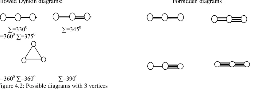
. It is also possible to present the information in the Cartan matrix in a graphical way via Dynkin diagrams.

C. CLASSIfiCATION OF CONNECTED DYNKIN DIAGRAMS

Dynkin diagrams are a very effective tool for classifying simple root systems

S

, and consequently the reduced root systems

R

. Since reducible root systems are a disjoint union of mutually orthogonal subroot systems, the Dynkin diagram is just drawn out of many connected graphs. It is thus sufficient to classify connected Dynkin diagrams which will help to state the result of this classification and as well as to sketch a simplified proof.

Theorem 4.4 (Classification of Dynkin diagrams).

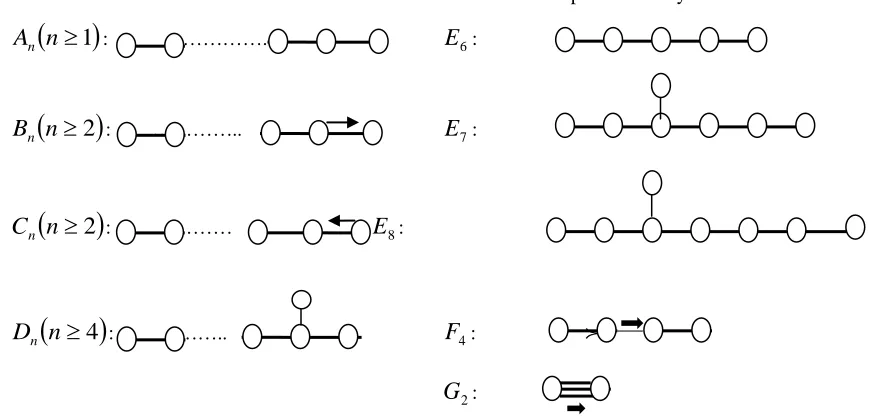
Let

R

be a reduced irreducible root system. Then its Dynkin diagram is isomorphic to a diagram from the figure below, which is also equipped with labels of the diagrams. The index in the label is always equal to the number of simple roots, and each of the diagrams is realized for some reduced irreducible root system

R

.

The Families The 5 exceptional root systems



n



1



A

_n : ………….

E

₆:



n



2



B

_n : …………..

E

₇:



n



2



C

_n : : ………

E

8:



n



4



D

_n : ……..

F

₄: ≻

2

G

:

ISSN: 2231-5373

http://www.ijmttjournal.org

Page 194

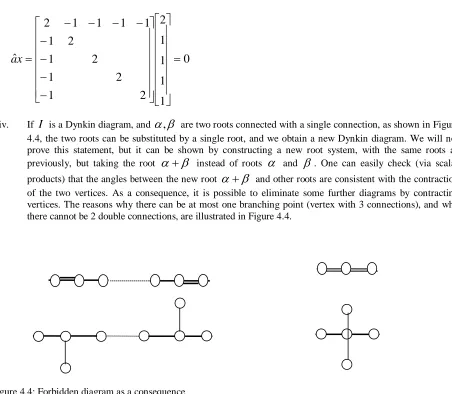
We now turn to a simplified proof of the theorem. It turns out that all irreducible simple root systems in the figure above can indeed be constructed. In the process of this work we shall see the reason why diagrams with different connections are not valid as Dynkin diagrams of simple root systems. Only connected graphs of vertices with either a null, single, dual or triple connection with another vertex will be considered. The Dynkin diagrams as graphs of an irreducible simple root systems are a subset of all possible graphs under consideration. Before we start, an important notion has to be introduced i.e. the subgraph. If

I

is the set of vertices of a graph, then a subgraph consists of a subset of vertices

J



I

, while the types of connections between the vertices in

J

stay the same as in the original graph

I

. Also, a special case of a Dynkin diagram is a graph

I

, which contains no dual or triple connections. For the purposes of this work, we shall call such a diagram a simple graph. A number of the properties of Dynkin diagrams can be deduced by looking at subgraphs. Suppose we have a true Dynkin diagram

I

as a realization of an irreducible simple root system. This diagram contains all the necessary information for the construction of the Cartanmatrix

a

_ij. If the root system spans a

n

-dimensional vector space

V

, then the

n

roots constitute a basis of this space, and the Cartan matrix is a linear operator on the vector space

V

.

this operator is written as a matrix in the basis

 



_{i iI}

.

Suppose we have a subgraph of this Dynkin diagram, we specify a subset

J

of simple root vectors



_i

:

i



J

(for a given labeling of the simple roots). If the chosen number of simple roots is

K

then the subgraph

J

has

K

vertices, and we can construct a

K



K

submatrix of the Cartan matrix with entries

a

ij, where

i

,

j



J

. This matrix can be again viewed as a linear operator, this time on the space

V

, which is spanned by the roots



_j with

j



J

. The linear operator



a

, constructed by choosing a subset of indices

J

from the Cartan matrix, is always positive definite which means

0

,

















x

x

a

for all

x



V

\

 

0

. Indeed, if





_ J j

c

j j

x



, then





_





_



_

_





















      













































J

j j j

j J k j k k J

j i J

j i i j j J k j i k j j j j i k i J k j i k k j ij i

x

c

c

c

c

c

a

c

x

x

a

.

0

,

,

2

,

,

,

2

,

,

,

2

,

,

2 , , , ,





































The result (which is a sum of nonnegative terms) cannot be zero, because that would imply that



x

,



j





0

for all

J

j



and therefore

x

would be orthogonal to all

a

_j. This is not possible, since

x

is a nonzero vector in

V

and

vectors



_j for

j



J

form a basis of the vectorspace

V

that means that given any subgraph

J

of a given diagram, its Cartan matrix is positive definite. This will allow us to put restrictions, on what kind of subgraphs can be found in the Dynkin diagrams.

Here are some important rules as a motivation for the classification theorem.