Laplace Transforms: Theory, Problems, and
Solutions
Marcel B. Finan
Arkansas Tech University
c
Contents
43 The Laplace Transform: Basic Definitions and Results 3
44 Further Studies of Laplace Transform 15
45 The Laplace Transform and the Method of Partial Fractions 28
46 Laplace Transforms of Periodic Functions 35
47 Convolution Integrals 45
48 The Dirac Delta Function and Impulse Response 53
49 Solving Systems of Differential Equations Using Laplace
Trans-form 61
43
The Laplace Transform: Basic Definitions
and Results
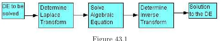
Laplace transform is yet another operational tool for solving constant coeffi-cients linear differential equations. The process of solution consists of three main steps:
• The given “hard” problem is transformed into a “simple” equation. • This simple equation is solved by purely algebraic manipulations.
• The solution of the simple equation is transformed back to obtain the so-lution of the given problem.
In this way the Laplace transformation reduces the problem of solving a dif-ferential equation to an algebraic problem. The third step is made easier by tables, whose role is similar to that of integral tables in integration.
The above procedure can be summarized by Figure 43.1
Figure 43.1
In this section we introduce the concept of Laplace transform and discuss some of its properties.
The Laplace transform is defined in the following way. Let f(t) be defined for t ≥ 0. Then the Laplace transform of f, which is denoted by L[f(t)] or by F(s), is defined by the following equation
L[f(t)] = F(s) = lim
T→∞ Z T
0
f(t)e−stdt =
Z ∞
0
f(t)e−stdt
The integral which defined a Laplace transform is an improper integral. An improper integral may converge or diverge, depending on the integrand. When the improper integral in convergent then we say that the function f(t) possesses a Laplace transform. So what types of functions possess Laplace transforms, that is, what type of functions guarantees a convergent improper integral.
Example 43.1
Find the Laplace transform, if it exists, of each of the following functions
Solution.
(a) Using the definition of Laplace transform we see that
L[eat] =
Z ∞
0
e−(s−a)tdt= lim
T→∞ Z T
0
e−(s−a)tdt.
But
Z T
0
e−(s−a)tdt=
T if s=a
1−e−(s−a)T
s−a if s6=a.
For the improper integral to converge we need s > a. In this case,
L[eat] =F(s) = 1
s−a, s > a.
(b) In a similar way to what was done in part (a), we find
L[1] =
Z ∞
0
e−stdt= lim
T→∞ Z T
0
e−stdt= 1
s, s >0.
(c) We have
L[t] =
Z ∞
0
te−stdt =
−te
−st
s − e−st
s2
∞
0
= 1
s2, s >0.
(d) Again using the definition of Laplace transform we find
L[et2] =
Z ∞
0
et2−stdt.
Ifs≤0 thent2−st≥0 so thatet2−st
≥1 and this implies thatR∞
0 e
t2−st
dt≥
R∞
0 .Since the integral on the right is divergent, by the comparison theorem
of improper integrals (see Theorem 43.1 below) the integral on the left is also divergent. Now, if s > 0 then R∞
0 e
t(t−s)dt ≥ R∞
s dt. By the same reasoning
the integral on the left is divergent. This shows that the function f(t) =et2
does not possess a Laplace transform
The above example raises the question of what class or classes of functions possess a Laplace transform. Looking closely at Example 43.1(a), we notice that for s > athe integral R0∞e−(s−a)tdt is convergent and a critical
compo-nent for this convergence is the type of the functionf(t).To be more specific, if f(t) is a continuous function such that
where M ≥0 and a and C are constants, then this condition yields
Z ∞
0
f(t)e−stdt≤
Z C
0
f(t)e−stdt+M
Z ∞
C
e−(s−a)tdt.
Sincef(t) is continuous in 0≤t≤C,by lettingA= max{|f(t)|: 0≤t≤C} we have
Z C
0
f(t)e−stdt≤A
Z C
0
e−stdt =A
1
s − e−sC
s
<∞.
On the other hand, Now, by Example 43.1(a), the integral RC∞e−(s−a)tdt is
convergent for s > a. By the comparison theorem of improper integrals (see Theorem 43.1 below) the integral on the left is also convergent. That is, f(t) possesses a Laplace transform.
We call a function that satisfies condition (1) a function with anexponential order at infinity. Graphically, this means that the graph off(t) is contained in the region bounded by the graphs of y =M eat and y=−M eat for t≥C.
Note also that this type of functions controls the negative exponential in the transform integral so that to keep the integral from blowing up. If C = 0 then we say that the function is exponentially bounded.
Example 43.2
Show that any bounded function f(t) for t≥0 is exponentially bounded.
Solution.
Since f(t) is bounded for t ≥ 0, there is a positive constant M such that |f(t)| ≤ M for all t ≥0. But this is the same as (1) with a = 0 and C = 0.
Thus, f(t) has is exponentially bounded
Another question that comes to mind is whether it is possible to relax the condition of continuity on the function f(t).Let’s look at the following situ-ation.
Example 43.3
Figure 43.2
Note that the function is periodic of period 2.
Solution.
Sincef(t)e−st ≤e−st,we haveR∞
0 f(t)e
−stdt ≤R∞
0 e
−stdt.But the integral on
the right is convergent for s >0 so that the integral on the left is convergent as well. That is, L[f(t)] exists for s >0
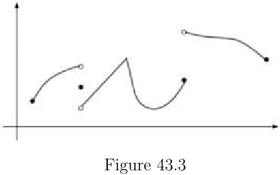
The function of the above example belongs to a class of functions that we define next. A function is called piecewise continuous on an interval if the interval can be broken into a finite number of subintervals on which the function is continuous on each open subinterval (i.e. the subinterval without its endpoints) and has a finite limit at the endpoints (jump discontinuities and no vertical asymptotes) of each subinterval. Below is a sketch of a piecewise continuous function.
Figure 43.3
Note that a piecewise continuous function is a function that has a finite number of breaks in it and doesnt blow up to infinity anywhere. A function defined for t ≥0 is said to be piecewise continuous on the infinite in-terval if it is piecewise continuous on 0≤t≤T for all T >0.
Example 43.4
(a) f(t) =tn (b) f(t) = tnsinat
Solution.
(a) Since et =P∞ n=0
tn n! ≥
tn
n!, we have t
n ≤ n!et. Hence, tn is piecewise
con-tinuous and exponentially bounded.
(b) Since |tnsinat| ≤ n!et, we have tnsinat is piecewise continuous and ex-ponentially bounded
Next, we would like to establish the existence of the Laplace transform for all functions that are piecewise continuous and have exponential order at infinity. For that purpose we need the following comparison theorem from calculus.
Theorem 43.1
Suppose that f(t) and g(t) are both integrable functions for all t ≥ t0 such
that |f(t)| ≤ |g(t) for t ≥ t0. If
R∞
t0 g(t)dt is convergent, then
R∞
t0 f(t)dt is
also convergent. If, on the other hand,Rt∞
0 f(t)dt is divergent then
R∞
t0 f(t)dt
is also divergent.
Theorem 43.2 (Existence)
Suppose that f(t) is piecewise continuous on t ≥ 0 and has an exponential order at infinity with |f(t)| ≤M eat for t ≥C.Then the Laplace transform
F(s) =
Z ∞
0
f(t)e−stdt
exists as long as s > a.Note that the two conditions above are sufficient, but not necessary, for F(s) to exist.
Proof.
The integral in the definition of F(s) can be splitted into two integrals as follows
Z ∞
0
f(t)e−stdt=
Z C
0
f(t)e−stdt+
Z ∞
C
f(t)e−stdt.
Since f(t) is piecewise continuous in 0 ≤ t ≤ C, it is bounded there. By letting A= max{|f(t)|: 0≤t ≤C} we have
Z C
0
f(t)e−stdt≤A
Z C
0
e−stdt =A
1
s − e−sC
s
Now, by Example 43.1(a), the integral RC∞f(t)e−stdt is convergent fors > a.
By Theorem 43.1 the integral on the left is also convergent. That is, f(t) possesses a Laplace transform
In what follows, we will denote the class of all piecewise continuous func-tions with exponential order at infinity byPE. The next theorem shows that any linear combination of functions inPE is also inPE.The same is true for the product of two functions in PE.
Theorem 43.3
Suppose that f(t) and g(t) are two elements of PE with
|f(t)| ≤M1ea1t, t≥C1 and |g(t)| ≤M2ea1t, t ≥C2.
(i) For any constants α andβ the functionαf(t) +βg(t) is also a member of PE. Moreover
L[αf(t) +βg(t)] =αL[f(t)] +βL[g(t)].
(ii) The function h(t) =f(t)g(t) is an element of PE.
Proof.
(i) It is easy to see that αf(t) +βg(t) is a piecewise continuous function. Now, let C =C1+C2, a= max{a1, a2}, and M =|α|M1+|β|M2.Then for t ≥C we have
|αf(t) +βg(t)| ≤ |α||f(t)|+|β||g(t)| ≤ |α|M1ea1t+|β|M2ea2t≤M eat.
This shows that αf(t) +βg(t) is of exponential order at infinity. On the other hand,
L[αf(t) +βg(t)] = limT→∞ RT
0 [αf(t) +βg(t)]dt
= αlimT→∞ RT
0 f(t)dt+βlimT→∞
RT
0 g(t)dt
= αL[f(t)] +βL[g(t)]
(ii) It is clear that h(t) =f(t)g(t) is a piecewise continuous function. Now, lettingC =C1+C2, M =M1M2, anda=a1+a2 then we see that fort≥C
we have
Hence, h(t) is of exponential order at infinity. By Theorem 43.2 , L[h(t)] exists for s > a
We next discuss the problem of how to determine the function f(t) if F(s) is given. That is, how do we invert the transform. The following result on uniqueness provides a possible answer. This result establishes a one-to-one correspondence between the set PE and its Laplace transforms. Alterna-tively, the following theorem asserts that the Laplace transform of a member in PE is unique.
Theorem 43.4
Let f(t) and g(t) be two elements in PE with Laplace transforms F(s) and
G(s) such that F(s) = G(s) for some s > a. Then f(t) = g(t) for all t ≥ 0 where both functions are continuous.
The standard techniques used to prove this theorem( i.e., complex analysis, residue computations, and/or Fourier’s integral inversion theorem) are gen-erally beyond the scope of an introductory differential equations course. The interested reader can find a proof in the book ”Operational Mathematics” by Ruel Vance Churchill or in D.V. Widder ”The Laplace Transform”. With the above theorem, we can now officially define the inverse Laplace transform as follows: For a piecewise continuous function f of exponential order at infinity whose Laplace transform isF,we callf theinverse Laplace transform of F and write f =L−1[F(s)]. Symbolically
f(t) =L−1[F(s)]⇐⇒F(s) = L[f(t)].
Example 43.5 Find L−1 1
s−1
, s > 1.
Solution.
From Example 43.1(a), we have that L[eat] = s−1a, s > a. In particular, for
a= 1 we find that L[et] = 1
s−1, s >1. Hence, L
−1 1
s−1
=et, t≥0 .
The above theorem states that iff(t) is continuous and has a Laplace trans-form F(s), then there is no other function that has the same Laplace trans-form. To find L−1[F(s)], we can inspect tables of Laplace transforms of
known functions to find a particular f(t) that yields the given F(s).
Laplace transform is not assured. The following example addresses the uniqueness issue.
Example 43.6
Consider the two functions f(t) = h(t)h(3−t) and g(t) =h(t)−h(t−3).
(a) Are the two functions identical? (b) Show that L[f(t)] =L[g(t).
Solution. (a) We have
f(t) =
1, 0≤t≤3 0, t >3 and
g(t) =
1, 0≤t <3 0, t≥3
So the two functions are equal for all t6= 3 and so they are not identical. (b) We have
L[f(t)] =L[g(t)] =
Z 3
0
e−stdt= 1−e
−3s
s , s >0.
Thus, both functions f(t) and g(t) have the same Laplace transform even though they are not identical. However, they are equal on the interval(s) where they are both continuous
The inverse Laplace transform possesses a linear property as indicated in the following result.
Theorem 43.5
Given two Laplace transforms F(s) and G(s) then
L−1[aF(s) +bG(s)] =aL−1[F(s)] +bL−1[G(s)]
for any constants a and b.
Proof.
Suppose that L[f(t)] = F(s) and L[g(t)] = G(s). Since L[af(t) +bg(t)] =
Practice Problems
Problem 43.1
Determine whether the integral R0∞1+1t2dt converges. If the integral
con-verges, give its value.
Problem 43.2
Determine whether the integral R∞
0
t
1+t2dt converges. If the integral
con-verges, give its value.
Problem 43.3
Determine whether the integral R0∞e−tcos (e−t)dt converges. If the integral converges, give its value.
Problem 43.4
Using the definition, find L[e3t], if it exists. If the Laplace transform exists
then find the domain of F(s).
Problem 43.5
Using the definition, find L[t−5],if it exists. If the Laplace transform exists then find the domain of F(s).
Problem 43.6
Using the definition, find L[e(t−1)2
], if it exists. If the Laplace transform exists then find the domain of F(s).
Problem 43.7
Using the definition, find L[(t −2)2], if it exists. If the Laplace transform exists then find the domain of F(s).
Problem 43.8
Using the definition, find L[f(t)],if it exists. If the Laplace transform exists then find the domain of F(s).
f(t) =
0, 0≤t <1
Problem 43.9
Using the definition, find L[f(t)],if it exists. If the Laplace transform exists then find the domain of F(s).
f(t) =
0, 0≤t <1
t−1, 1≤t <2 0, t ≥2.
Problem 43.10
Letnbe a positive integer. Using integration by parts establish the reduction formula
Z
tne−stdt=−t
ne−st
s + n s
Z
tn−1e−stdt, s >0.
Problem 43.11
For s >0 andn a positive integer evaluate the limits
limt→0tne−st (b) limt→∞tne−st
Problem 43.12
(a) Use the previous two problems to derive the reduction formula for the Laplace transform of f(t) = tn,
L[tn] = n
sL[t
n−1], s >0.
(b) Calculate L[tk],for k = 1,2,3,4,5.
(c) Formulate a conjecture as to the Laplace transform of f(t), tn with n a positive integer.
From a table of integrals,
R
eαusinβudu = eαu αsinβu−βsinβu α2+β2
R
eαucosβudu = eαu αcosβu+βsinβu α2+β2
Problem 43.13
Use the above integrals to find the Laplace transform of f(t) = cosωt, if it exists. If the Laplace transform exists, give the domain of F(s).
Problem 43.14
Problem 43.15
Use the above integrals to find the Laplace transform of f(t) = cosω(t−2),
if it exists. If the Laplace transform exists, give the domain of F(s).
Problem 43.16
Use the above integrals to find the Laplace transform of f(t) = e3tsint, if it
exists. If the Laplace transform exists, give the domain of F(s).
Problem 43.17
Use the linearity property of Laplace transform to find L[5e−7t+t+ 2e2t].
Find the domain of F(s).
Problem 43.18
Consider the function f(t) = tant.
(a) Is f(t) continuous on 0 ≤ t < ∞, discontinuous but piecewise contin-uous on 0≤t <∞, or neither?
(b) Are there fixed numbersaandM such that|f(t)| ≤M eat for 0≤t <∞?
Problem 43.19
Consider the function f(t) = t2e−t.
(a) Is f(t) continuous on 0 ≤ t < ∞, discontinuous but piecewise contin-uous on 0≤t <∞, or neither?
(b) Are there fixed numbersaandM such that|f(t)| ≤M eat for 0≤t <∞?
Problem 43.20
Consider the function f(t) = et
2
e2t+1.
(a) Is f(t) continuous on 0 ≤ t < ∞, discontinuous but piecewise contin-uous on 0≤t <∞, or neither?
(b) Are there fixed numbersaandM such that|f(t)| ≤M eat for 0≤t <∞?
Problem 43.21
Consider the floor function f(t) = btc, where for any integer n we have btc=n for all n≤t < n+ 1.
(a) Is f(t) continuous on 0 ≤ t < ∞, discontinuous but piecewise contin-uous on 0≤t <∞, or neither?
Problem 43.22 Find L−1 3
s−2
.
Problem 43.23 Find L−1 −2
s2 +
1
s+1
.
Problem 43.24 Find L−1 2
s+2 + 2
s−2
44
Further Studies of Laplace Transform
Properties of the Laplace transform enable us to find Laplace transforms without having to compute them directly from the definition. In this sec-tion, we establish properties of Laplace transform that will be useful for solving ODEs.
Laplace Transform of the Heaviside Step Function
The Heaviside step function is a piecewise continuous function defined by
h(t) =
1, t≥0 0, t <0
Figure 44.1 displays the graph of h(t).
Figure 44.1
Taking the Laplace transform of h(t) we find
L[h(t)] =
Z ∞
0
h(t)e−stdt =
Z ∞
0
e−stdt =
−e
−st
s
∞
0
= 1
s, s >0.
A Heaviside function atα ≥0 is the shifted functionh(t−α) (α units to the right). For this function, the Laplace transform is
L[h(t−α)] =
Z ∞
0
h(t−α)e−stdt=
Z ∞
α
e−stdt =
−e
−st
s
∞
α
= e
−sα
s , s >0.
Laplace Tranform of eat
The Laplace transform for the function f(t) = eat is
L[eat] =
Z ∞
0
e−(s−a)tdt =
−e
−(s−a)t
s−a
∞
0
= 1
Laplace Tranforms of sinat and cosat
Using integration by parts twice we find
L[sinat] = R0∞e−stsinatdt
= h−e−stsinat
s −
ae−stcosat
s2
i∞
0
− a2
s2
R∞
0 e
−stsinatdt
= −a
s2 −
a2
s2L[sinat]
s2+a2
s2
L[sinat] = sa2
L[sinat] = s2+aa2, s > 0
A similar argument shows that
L[cosat] = s
s2+a2, s > 0.
Laplace Transforms of coshat and sinhat
Using the linear property of L we can write
L[coshat] = 12(L[eat] +L[e−at])
= 1
2 1
s−a+
1
s+a
, s > |a|
= s2−sa2, s > |a|
A similar argument shows that
L[sinat] = a
s2−a2, s > |a|.
Laplace Transform of a Polynomial
Let n be a positive integer. Using integration by parts we can write
Z ∞
0
tne−stdt =−
tne−st s
∞
0
+n
s
Z ∞
0
tn−1e−stdt.
By repeated use of L’Hˆopital’s rule we find limt→∞tne−st = limt→∞ snne!st = 0
for s >0. Thus,
L[tn] = n
sL[t
n−1
Using induction on n = 0,1,2,· · · one can easily eastablish that
L[tn] = n!
sn+1, s >0.
Using the above result together with the linearity property of L one can find the Laplace transform of any polynomial.
The next two results are referred to as the first and second shift theorems. As with the linearity property, the shift theorems increase the number of functions for which we can easily find Laplace transforms.
Theorem 44.1 (First Shifting Theorem)
Iff(t) is a piecewise continuous function fort≥0 and has exponential order at infinity with |f(t)| ≤M eat, t≥C,then for any real number α we have
L[eαtf(t)] =F(s−α), s > a+α
where L[f(t)] =F(s).
Proof.
From the definition of the Laplace transform we have
L[eatf(t)] =
Z ∞
0
e−steatf(t)dt =
Z ∞
0
e−(s−a)tf(t)dt.
Using the change of variable β =s−a the previous equation reduces to
L[eatf(t)] =
Z ∞
0
e−steatf(t)dt =
Z ∞
0
e−βtf(t)dt =F(β) =F(s−a), s > a+α
Theorem 44.2 (Second Shifting Theorem)
Iff(t) is a piecewise continuous function fort≥0 and has exponential order at infinity with |f(t)| ≤ M eat, t ≥ C, then for any real number α ≥ 0 we
have
L[f(t−α)h(t−α)] =e−αsF(s), s > a
where L[f(t)] =F(s) and h(t) is the Heaviside step function.
Proof.
From the definition of the Laplace transform we have
L[f(t−α)h(t−α)] =
Z ∞
0
f(t−α)h(s−α)e−stdt=
Z ∞
α
Using the change of variable β =t−α the previous equation reduces to L[f(t−α)h(t−α)] = R∞
0 f(β)e
−s(β+α)dβ
= e−sαR0∞f(β)e−sβdβ =e−sαF(s), s > a
Example 44.1 Find
(a) L[e2tt2] (b) L[e3tcos 2t] (c) L−1[e−2ts2]
Solution.
(a) By Theorem 44.1, we have L[e2tt2] = F(s − 2) where L[t2] = 2!
s3 =
F(s), s >0. Thus,L[e2tt2] = (s−22)3, s >2.
(b) As in part (a), we haveL[e3tcos 2t] =F(s−3) whereL[cos 2t] =F(s−3).
But L[cos 2t] = s2s+4, s >0. Thus,
L[e3tcos 2t] = s−3
(s−3)2+ 4, s >3
(c) Since L[t] = s12, by Theorem 44.2, we have
e−2t
s2 =L[(t−2)h(t−2)].
Therefore,
L−1
e−2t
s2
= (t−2)h(t−2) =
0, 0≤t <2
t−2, t≥2
The following result relates the Laplace transform of derivatives and integrals to the Laplace transform of the function itself.
Theorem 44.3
Suppose that f(t) is continuous for t ≥ 0 and f0(t) is piecewise continuous of exponential order at infinity with |f0(t)| ≤M eat, t≥C Then
(a) f(t) is of exponential order at infinity.
(b) L[f0(t)] =sL[f(t)]−f(0) = sF(s)−f(0), s >max{a,0}+ 1.
(c) L[f00(t)] = s2L[f(t)] − sf(0) − f0(0) = s2F(s) − sf(0) − f(0), s >
max{a,0}+ 1.
(d) LhRt
0 f(u)du
i
Proof.
(a) By the Fundamental Theorem of Calculus we havef(t) = f(0)−Rt
0 f
0(u)du.
Also, since f0 is piecewise continuous, |f0(t)| ≤ T for some T > 0 and all 0≤t≤C. Thus,
|f(t)| =
f(0)− Rt
0 f
0(u)du
=|f(0)− RC
0 f
0(u)du−Rt
Cf
0(u)du|
≤ |f(0)|+T C +MRt
Ce audu
Note that if a >0 then
Z t
C
eaudu= 1
a(e
at−
eaC)≤ e
at
a
and so
|f(t)| ≤[|f(0)|+T C +M
a ]e
at.
If a= 0 then
Z t
C
eaudu=t−C
and therefore
|f(t)| ≤ |f(0)|+T C +M(t−C)≤(|f(0)|+T C +M)et.
Now, if a <0 then
Z t
C
eaudu= 1
a(e
at−eaC)≤ 1
|a|
so that
|f(t)| ≤(|f(0)|+T C +M |a|)e
t
It follows that
|f(t)| ≤N ebt, t≥0 where b= max{a,0}+ 1.
(b) From the definition of Laplace transform we can write
L[f0(t)] = lim
A→∞ Z A
0
Since f0(t) may have jump discontinuities at t1, t2,· · · , tN in the interval
0≤t≤A, we can write
Z A
0
f0(t)e−stdt =
Z t1
0
f0(t)e−stdt+
Z t2
t1
f0(t)e−stdt+· · ·+
Z A
tN
f0(t)e−stdt.
Integrating each term on the RHS by parts and using the continuity of f(t) to obtain
Rt1
0 f
0
(t)e−stdt = f(t1)e−st1 −f(0) +sRt1
0 f(t)e
−stdt
Rt2
t1 f
0(t)e−stdt = f(t
2)e−st2 −f(t1)e−st1 +s
Rt2
t1 f(t)e
−stdt
.. .
RtN
tN−1f
0(t)e−stdt = f(t
N)e−stN −f(tN−1)e−stN−1 +s
RtN
tN−1f(t)e
−stdt
RA
tNf
0(t)e−stdt = f(A)e−sA−f(t
N)e−stN +s
RA
tNf(t)e
−stdt
Also, by the continuity of f(t) we can write
Z A
0
f(t)e−stdt =
Z t1
0
f(t)e−stdt+
Z t2
t1
f(t)e−stdt+· · ·+
Z A
tN
f(t)e−stdt.
Hence,
Z A
0
f0(t)e−stdt =f(A)e−sA−f(0) +s
Z A
0
f(t)e−stdt.
Since f(t) has exponential order at infinity,limA→∞f(A)e−sA = 0. Hence,
L[f0(t)] = sL[f(t)]−f(0).
(c) Using part (b) we find
L[f00(t)] = sL[f0(t)]−f0(0) = s(sF(s)−f(0))−f0(0)
= s2F(s)−sf(0)−f0(0), s > max{a,0}+ 1
(d) Since dtd
Rt
0 f(u)du
=f(t), by part (b) we have
F(s) =L[f(t)] =sL
Z t
0
f(u)du
and therefore
L
Z t
0
f(u)du
= L[f(t)]
s = F(s)
s , s > max{a,0}+ 1
The argument establishing part (b) of the previous theorem can be extended to higher order derivatives.
Theorem 44.4
Let f(t), f0(t),· · · , f(n−1)(t) be continuous and f(n)(t) be piecewise
continu-ous of exponential order at infinity with |f(n)(t)| ≤M eat, t≥C. Then
L[f(n)(t)] =snL[f(t)]−sn−1f(0)−sn−2f0(0)−· · ·−f(n−1)(0), s >max{a,0}+1.
We next illustrate the use of the previous theorem in solving initial value problems.
Example 44.2
Solve the initial value problem
y00−4y0+ 9y=t, y(0) = 0, y0(0) = 1.
Solution.
We apply Theorem 44.4 that gives the Laplace transform of a derivative. By the linearity property of the Laplace transform we can write
L[y00]−4L[y0] + 9L[y] =L[t].
Now since
L[y00] = s2L[y]−sy(0)−y0(0) =s2Y(s)−1 L[y0] = sY(s)−y(0) = sY(s)
L[t] = s12
where L[y] =Y(s), we obtain
s2Y(s)−1−4sY(s) + 9Y(s) = 1
s2.
Rearranging gives
(s2−4s+ 9)Y(s) = s
2+ 1
Thus,
Y(s) = s
2+ 1
s2(s2−4s+ 9)
and
y(t) = L−1
s2+ 1
s2(s2−4s+ 9)
In the next section we will discuss a method for finding the inverse Laplace transform of the above expression.
Example 44.3
Consider the mass-spring oscillator without friction: y00 +y = 0. Suppose we add a force which corresponds to a push (to the left) of the mass as it oscillates. We will suppose the push is described by the function
f(t) =−h(t−2π) +u(t−(2π+a))
for some a > 2π which we are allowed to vary. (A small a will correspond to a short duration push and a large a to a long duration push.) We are interested in solving the initial value problem
y00+y=f(t), y(0) = 1, y0(0) = 0.
Solution.
To begin, determine the Laplace transform of both sides of the DE:
L[y00+y] =L[f(t)]
or
s2Y −sy(0)−y0(0) +Y(s) =−1
se
−2πs+ 1
se
−(2π+a)s.
Thus,
Y(s) = e
−(2π+a)s
s(s2 + 1) −
e−2πs s(s2+ 1) +
s s2+ 1.
Now since s(s21+1) =
1
s − s
s2+1 we see that
Y(s) = e−(2π+a)s
1
s − s s2+ 1
−e−2πs
1
s − s s2+ 1
+ s
and therefore
y(t) = h(t−(2π+a))L−1 1
s − s s2+1
(t−(2π+a)) − h(t−2π)L−1 1
s − s s2+1
(t−2π) + cost
= h(t−(2π+a))[1−cos (t−(2π+a))]−u(t−2π)[1−cos (t−2π)]
+ cost
We conclude this section with the following table of Laplace transform pairs.
f(t) F(s)
h(t) =
1, t ≥0 0, t <0
1
s, s >0
tn, n= 1,2,· · · n!
sn+1, s >0
eαt s
s−α, s > α
sin (ωt) s2+ωω2, s >0
cos (ωt) s
s2+ω2, s >0
sinh (ωt) s2−ωω2, s >|ω|
cosh (ωt) s2−sω2, s >|ω|
eαtf(t), with |f(t)| ≤M eat F(s−α), s > α+a
eαth(t) s−1α, s > α
eαttn, n = 1,2,· · · n!
(s−α)n+1, s > α
eαtsin (ωt) ω
(s−α)2+ω2, s > α
eαtcos (ωt) s−α
(s−α)2+ω2, s > α
f(t−α)h(t−α), α≥0 e−αsF(s), s > a
f(t) F(s) (continued)
h(t−α), α≥0 e−sαs, s >0
tf(t) -F0(s)
t
2ωsinωt
s
(s2+ω2)2, s >0
1
2ω3[sinωt−ωtcosωt]
1
(s2+ω2)2, s >0
f0(t), with f(t) continuous sF(s)−f(0)
and|f0(t)| ≤M eat s >max{a,0}+ 1
f00(t), with f0(t)continuous s2F(s)−sf(0)−f0(0)
and|f00(t)| ≤M eat s >max{a,0}+ 1
f(n)(t), with f(n−1)(t) continuous snF(s)−sn−1f(0)− · · · and|f(n)(t)| ≤M eat -sf(n−2)(0)−f(n−1)(0)
s >max{a,0}+ 1
Rt
0 f(u)du, with |f(t)| ≤M e
at F(s)
s , s >max{a,0}+ 1
Practice Problems
Problem 44.1
Use Table L to findL[2et+ 5].
Problem 44.2
Use Table L to findL[e3t−3h(t−1)].
Problem 44.3
Use Table L to findL[sin2ωt].
Problem 44.4
Use Table L to findL[sin 3tcos 3t].
Problem 44.5
Use Table L to findL[e2tcos 3t].
Problem 44.6
Use Table L to findL[e4t(t2+ 3t+ 5)].
Problem 44.7
Use Table L to findL−1[ 10
s2+25 +
4
s−3].
Problem 44.8
Use Table L to findL−1[ 5 (s−3)4].
Problem 44.9
Use Table L to findL−1[e−2s
s−9].
Problem 44.10
Use Table L to findL−1[e−3s(2s+7)
s2+16 ].
Problem 44.11
Graph the function f(t) = h(t−1) +h(t−3) for t ≥ 0, where h(t) is the Heaviside step function, and use Table L to findL[f(t)].
Problem 44.12
Problem 44.13
Graph the function f(t) = 3[h(t−1)−h(t−4)] for t≥ 0, where h(t) is the Heaviside step function, and use Table L to findL[f(t)].
Problem 44.14
Graph the function f(t) =|2−t|[h(t−1)−h(t−3)] for t≥0,where h(t) is the Heaviside step function, and use Table L to find L[f(t)].
Problem 44.15
Graph the functionf(t) = h(2−t) fort≥0,whereh(t) is the Heaviside step function, and use Table L to findL[f(t)].
Problem 44.16
Graph the function f(t) = h(t−1) +h(4−t) for t ≥ 0, where h(t) is the Heaviside step function, and use Table L to findL[f(t)].
Problem 44.17
The graph of f(t) is given below. Represent f(t) as a combination of Heav-iside step functions, and use Table L to calculate the Laplace transform of
f(t).
Problem 44.18
The graph of f(t) is given below. Represent f(t) as a combination of Heav-iside step functions, and use Table L to calculate the Laplace transform of
Problem 44.19
Using the partial fraction decomposition find L−1h 12 (s−3)(s+1)
i
.
Problem 44.20
Using the partial fraction decomposition find L−1h24e−5s s2−9
i
.
Problem 44.21
Use Laplace transform technique to solve the initial value problem
y0+ 4y=g(t), y(0) = 2
where
g(t) =
0, 0≤t <1 12, 1≤t <3
0, t ≥3
Problem 44.22
Use Laplace transform technique to solve the initial value problem
y00−4y=e3t, y(0) = 0, y0(0) = 0.
Problem 44.23
Obtain the Laplace transform of the functionR
45
The Laplace Transform and the Method
of Partial Fractions
In the last example of the previous section we encountered the equation
y(t) = L−1
s2+ 1
s2(s2−4s+ 9)
.
We would like to find an explicit expression for y(t). This can be done using the method of partial fractions which is the topic of this section. According to this method, finding L−1N(s)
D(s)
, where N(s) and D(s) are polynomials, require decomposing the rational function into a sum of simpler expressions whose inverse Laplace transform can be recognized from a table of Laplace transform pairs.
The method of integration by partial fractions is a technique for integrating rational functions, i.e. functions of the form
R(s) = N(s)
D(s) where N(s) and D(s) are polynomials.
The idea consists of writing the rational function as a sum of simpler frac-tions called partial fractions. This can be done in the following way:
Step 1. Use long division to find two polynomials r(s) and q(s) such that
N(s)
D(s) =q(s) +
r(s)
D(s).
Note that if the degree of N(s) is smaller than that of D(s) then q(s) = 0 and r(s) =N(s).
Step 2. Write D(s) as a product of factors of the form (as+b)n or (as2+
bs+c)n whereas2+bs+cis irreducible, i.e. as2+bs+c= 0 has no real zeros.
Step 3. Decompose Dr((ss)) into a sum of partial fractions in the following way:
(1) For each factor of the form (s−α)k write
A1 s−α +
A2
(s−α)2 +· · ·+ Ak
where the numbers A1, A2,· · · , Ak are to be determined.
(2) For each factor of the form (as2+bs+c)k write
B1s+C1 as2+bs+c+
B2s+C2
(as2+bs+c)2 +· · ·+
Bks+Ck
(as2+bs+c)k,
where the numbers B1, B2,· · · , Bk and C1, C2,· · · , Ck are to be determined.
Step 4. Multiply both sides by D(s) and simplify. This leads to an ex-pression of the form
r(s) = a polynomial whose coefficients are combinations of Ai,Bi, and Ci.
Finally, we find the constants, Ai, Bi, and Ci by equating the coefficients of
like powers of s on both sides of the last equation.
Example 45.1
Decompose into partial fractions R(s) = s3s+2s−21+2.
Solution.
Step 1. s3s+2s−21+2 =s+ 1 +
s+3
s2−1.
Step 2. s2−1 = (s−1)(s+ 1).
Step 3. (s+1)(s+3s−1) = sA+1 +sB−1.
Step 4. Multiply both sides of the last equation by (s−1)(s+ 1) to obtain
s+ 3 =A(s−1) +B(s+ 1).
Expand the right hand side, collect terms with the same power of s, and identify coefficients of the polynomials obtained on both sides:
s+ 3 = (A+B)s+ (B−A).
Hence, A+B = 1 and B−A= 3.Adding these two equations gives B = 2.
Thus, A=−1 and so
s3+s2+ 2
s2−1 =s+ 1−
1
s+ 1 + 2
s−1.
Now, after decomposing the rational function into a sum of partial fractions all we need to do is to find the Laplace transform of expressions of the form
A
(s−α)n or
Bs+C
Example 45.2 Find L−1h 1
s(s−3)
i
.
Solution. We write
1
s(s−3) =
A s +
B s−3. Multiply both sides by s(s−3) and simplify to obtain
1 =A(s−3) +Bs
or
1 = (A+B)s−3A.
Now equating the coefficients of like powers of s to obtain −3A = 1 and
A+B = 0.Solving for A and B we find A =−1
3 and B = 1
3. Thus,
L−1h 1
s(s−3)
i
= −1
3L
−11
s
+ 13L−1 1
s−3
= −1
3h(t) + 1 3e
3t, t≥0
where h(t) is the Heaviside unit step function
Example 45.3 Find L−13s+6
s2+3s
.
Solution.
We factor the denominator and split the integrand into partial fractions:
3s+ 6
s(s+ 3) =
A s +
B s+ 3. Multiplying both sides by s(s+ 3) to obtain
3s+ 6 = A(s+ 3) +Bs
= (A+B)s+ 3A
Equating the coefficients of like powers ofxto obtain 3A= 6 andA+B = 3. Thus, A= 2 andB = 1. Finally,
L−1
3s+ 6
s2+ 3s
= 2L−1
1
s
+L−1
1
s+ 3
Example 45.4 Find L−1h s2+1
s(s+1)2
i
.
Solution.
We factor the denominator and split the rational function into partial frac-tions:
s2+ 1
s(s+ 1)2 = A
s + B s+ 1 +
C
(s+ 1)2.
Multiplying both sides by s(s+ 1)2 and simplifying to obtain
s2+ 1 = A(s+ 1)2 +Bs(s+ 1) +Cs
= (A+B)s2+ (2A+B+C)s+A.
Equating coefficients of like powers of s we find A = 1,2A+B +C = 0 and A+B = 1. Thus,B = 0 and C =−2. Now finding the inverse Laplace transform to obtain
L−1
s2+ 1 s(s+ 1)2
=L−1
1
s
−2L−1
1 (s+ 1)2
=h(t)−2te−t, t≥0.
Example 45.5
Use Laplace transform to solve the initial value problem
y00+ 3y0+ 2y=e−t, y(0) =y0(0) = 0.
Solution.
By the linearity property of the Laplace transform we can write
L[y00] + 3L[y0] + 2L[y] =L[e−t].
Now since
L[y00] = s2L[y]−sy(0)−y0(0) =s2Y(s)
L[y0] = sY(s)−y(0) =sY(s) L[e−t] = s+11
where L[y] =Y(s), we obtain
s2Y(s) + 3sY(s) + 2Y(s) = 1
Rearranging gives
(s2+ 3s+ 2)Y(s) = 1
s+ 1. Thus,
Y(s) = 1
(s+ 1)(s2+ 3s+ 2).
and
y(t) = L−1
1
(s+ 1)(s2+ 3s+ 2)
.
Using the method of partial fractions we can write
1
(s+ 1)(s2+ 3s+ 2) =
1
s+ 2 − 1
s+ 1 + 1 (s+ 1)2.
Thus,
y(t) =L−1
1
s+ 2
−L−1
1
s+ 1
+L−1
1 (s+ 1)2
Practice Problems
In Problems 45.1 - 45.4, give the form of the partial fraction expansion for
F(s).You need not evaluate the constants in the expansion. However, if the denominator has an irreducible quadratic expression then use the completing the square process to write it as the sum/difference of two squares.
Problem 45.1
F(s) = s
3+ 3s+ 1
(s−1)3(s−2)2.
Problem 45.2
F(s) = s
2+ 5s−3
(s2+ 16)(s−2).
Problem 45.3
F(s) = s
3−1
(s2+ 1)2(s+ 4)2.
Problem 45.4
F(s) = s
4+ 5s2+ 2s−9
(s2+ 8s+ 17)(s−2)2.
Problem 45.5 Find L−1h 1
(s+1)3
i
.
Problem 45.6 Find L−1 2s−3
s2−3s+2
.
Problem 45.7 Find L−1h4s2+s+1
s3+s
i
.
Problem 45.8 Find L−1h s2+6s+8
s4+8s2+16
i
Problem 45.9
Use Laplace transform to solve the initial value problem
y0+ 2y= 26 sin 3t, y(0) = 3.
Problem 45.10
Use Laplace transform to solve the initial value problem
y0+ 2y= 4t, y(0) = 3.
Problem 45.11
Use Laplace transform to solve the initial value problem
y00+ 3y0+ 2y = 6e−t, y(0) = 1, y0(0) = 2.
Problem 45.12
Use Laplace transform to solve the initial value problem
y00+ 4y= cos 2t, y(0) = 1, y0(0) = 1.
Problem 45.13
Use Laplace transform to solve the initial value problem
y00−2y0+y =e2t, y(0) = 0, y0(0) = 0.
Problem 45.14
Use Laplace transform to solve the initial value problem
y00+ 9y=g(t), y(0) = 1, y0(0) = 0 where
g(t) =
6, 0≤t < π
0, π ≤t <∞ Problem 45.15
Determine the constantsα, β, y0,and y00 so thatY(s) = 2s−1
s2+s+2 is the Laplace
transform of the solution to the initial value problem
y00+αy0+βy = 0, y(0) =y0, y0(0) =y00.
Problem 45.16
Determine the constants α, β, y0, andy00 so that Y(s) =
s
(s+1)2 is the Laplace
transform of the solution to the initial value problem
46
Laplace Transforms of Periodic Functions
In many applications, the nonhomogeneous term in a linear differential equa-tion is a periodic funcequa-tion. In this secequa-tion, we derive a formula for the Laplace transform of such periodic functions.
Recall that a functionf(t) is said to beT−periodicif we havef(t+T) = f(t) whenever t and t+T are in the domain of f(t). For example, the sine and cosine functions are 2π−periodic whereas the tangent and cotangent func-tions are π−periodic.
If f(t) is T−periodic for t≥0 then we define the function
fT(t) =
f(t), 0≤t≤T
0, t > T
The Laplace transform of this function is then
L[fT(t)] =
Z ∞
0
fT(t)e−stdt=
Z T
0
f(t)e−stdt.
The Laplace transform of a T−periodic function is given next.
Theorem 46.1
If f(t) is a T−periodic, piecewise continuous fucntion for t≥0 then
L[f(t)] = L[fT(t)]
1−e−sT, s > 0.
Proof.
Since f(t) is piecewise continuous, it is bounded on the interval 0 ≤t ≤T.
By periodicity, f(t) is bounded for t ≥0. Hence, it has an exponential order at infinity. By Theorem 43.2, L[f(t)] exists for s >0.Thus,
L[f(t)] =
Z ∞
0
f(t)e−stdt =
∞ X
n=0
Z T
0
fT(t−nT)h(t−nT)e−stdt,
where the last sum is the result of decomposing the improper integral into a sum of integrals over the constituent periods.
By the Second Shifting Theorem (i.e. Theorem 44.2) we have
Hence,
L[f(t)] =
∞ X
n=0
e−nT sL[fT(t)] =L[fT(t)]
∞ X
n=0 e−nT s
!
.
Since s > 0, it follows that 0 < e−nT s<1 so that the series P∞ n=0e
−nT s is a
convergent geoemetric series with limit 1−e1−sT.Therefore,
L[f(t)] = L[fT(t)]
1−e−sT, s > 0
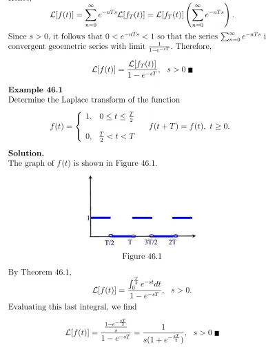
Example 46.1
Determine the Laplace transform of the function
f(t) =
1, 0≤t≤ T
2
f(t+T) = f(t), t≥0.
0, T2 < t < T
Solution.
The graph of f(t) is shown in Figure 46.1.
Figure 46.1
By Theorem 46.1,
L[f(t)] =
R T2
0 e
−stdt
1−e−sT , s > 0.
Evaluating this last integral, we find
L[f(t)] =
1−e−sT2
s
1−e−sT =
1
s(1 +e−sT2 )
, s >0
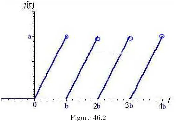
Example 46.2
Figure 46.2
Solution.
The given function is periodic of period b. For the first period the function is defined by
fb(t) =
a
bt[h(t)−h(t−b)].
So we have
L[fb(t)] = L[abt(h(t)−h(t−b))]
= −a
b d
dsL[h(t)−h(t−b)]
But
L[h(t)−h(t−b)] = L[h(t)]− L[h(t−b)]
= 1
s − e−bs
s , s >0
Hence,
L[fb(t)] =
a b
1
s2 −
bse−bs+e−bs
s2
.
Finally,
L[f(t)] = L[fb(t)] 1−e−bs =
a b
1−e−bs−bse−bs
s2(1−e−bs)
Example 46.3 Find L−1h1
s2 −
e−s
s(1−e−s)
i
.
Solution. Note first that
1
s2 −
e−s
s(1−e−s) =
1−e−s−se−s
According to the previous example with a = 1 and b = 1 we find that L−1h1
s2 −
e−s
s(1−e−s)
i
is the sawtooth function shown in Figure 46.2
Linear Time Invariant Systems and the Transfer Function
The Laplace transform is a powerful technique for analyzing linear time-invariant systems such as electrical circuits, harmonic oscillators, optical de-vices, and mechanical systems, to name just a few. A mathematical model described by a linear differential equation with constant coefficients of the form
any(n)+an−1y(n−1)+· · ·+a1y0+a0y=bmu(m)+bm−1u(m−1)+· · ·+b1u0+b0u
is called a linear time invariant system. The function y(t) denotes the system output and the functionu(t) denotes the system input. The system is called time-invariant because the parameters of the system are not changing over time and an input now will give the same result as the same input later. Applying the Laplace transform on the linear differential equation with null initial conditions we obtain
ansnY(s)+an−1sn−1Y(s)+· · ·+a0Y(s) =bmsmU(s)+bm−1sm−1U(s)+· · ·+b0U(s).
The function
Φ(s) = Y(s)
U(s) =
bmsm+bm−1sm−1 +· · ·+b1s+b0 ansn+an−1sn−1+· · ·+a1s+a0
is called the system transfer function. That is, the transfer function of a linear time-invariant system is the ratio of the Laplace transform of its output to the Laplace transform of its input.
Example 46.4
Consider the mathematical model described by the initial value problem
my00+γy0+ky =f(t), y(0) = 0, y0(0) = 0.
The coefficientsm, γ, and k describe the properties of some physical system, and f(t) is the input to the system. The solution y is the output at time t.
Solution.
By taking the Laplace transform and using the initial conditions we obtain
(ms2+γs+k)Y(s) =F(s).
Thus,
Φ(s) = Y(s)
F(s) =
1
ms2+γs+k (2)
Parameter Identification
One of the most useful applications of system transfer functions is for system or parameter identification.
Example 46.5
Consider a spring-mass system governed by
my00+γy0+ky =f(t), y(0) = 0, y0(0) = 0. (3)
Suppose we apply a unit step force f(t) = h(t) to the mass, initially at equilibrium, and you observe the system respond as
y(t) =−1 2e
−tcost−1
2e
−tsint+ 1
2. What are the physical parameters m, γ, and k?
Solution.
Start with the model (3)) withf(t) =h(t) and take the Laplace transform of both sides, then solve to findY(s) = s(ms2+1γs+k).Sincef(t) = h(t), F(s) =
1
s.
Hence
Φ(s) = Y(s)
F(s) =
1
ms2+γs+k.
On the other hand, for the input f(t) = h(t) the corresponding observed output is
y(t) =−1 2e
−t
cost−1 2e
−t
sint+ 1 2. Hence,
Y(s) = L[−1 2e
−tcost− 1 2e
−tsint+1 2]
= −1
2
s+1 (s+1)2+1 −
1 2
1 (s+1)2+1 +
1 2s
Thus,
Φ(s) = Y(s)
F(s) =
1
s2+ 2s+ 2.
Practice Problems
Problem 46.1
Find the Laplace transform of the periodic function whose graph is shown.
Problem 46.2
Find the Laplace transform of the periodic function whose graph is shown.
Problem 46.3
Problem 46.4
Find the Laplace transform of the periodic function whose graph is shown.
Problem 46.5
State the period of the function f(t) and find its Laplace transform where
f(t) =
sint, 0≤t < π
f(t+ 2π) = f(t), t≥0.
0, π≤t <2π
Problem 46.6
State the period of the function f(t) = 1−e−t, 0≤t <2, f(t+ 2) =f(t),
and find its Laplace transform.
Problem 46.7
Using Example 44.3 find
L−1
s2−s s3 +
e−s
s(1−e−s)
.
Problem 46.8
An object having massmis initially at rest on a frictionless horizontal surface. At time t= 0, a periodic force is applied horizontally to the object, causing it to move in the positive x-direction. The force, in newtons, is given by
f(t) =
f0, 0≤t≤ T2
f(t+T) =f(t), t≥0.
0, T2 < t < T
The initial value problem for the horizontal position, x(t), of the object is
(a) Use Laplace transforms to determine the velocity, v(t) = x0(t), and the position, x(t), of the object.
(b) Let m = 1 kg, f0 = 1 N, and T = 1 sec. What is the velocity, v, and position, x, of the object at t= 1.25 sec?
Problem 46.9
Consider the initial value problem
ay00+by0+cy=f(t), y(0) =y0(0) = 0, t >0
Suppose that the transfer function of this system is given by Φ(s) = 2s2+51s+2.
(a) What are the constants a, b, and c?
(b) If f(t) =e−t,determine F(s), Y(s), and y(t).
Problem 46.10
Consider the initial value problem
ay00+by0+cy=f(t), y(0) =y0(0) = 0, t >0
Suppose that an input f(t) =t, when applied to the above system produces the output y(t) = 2(e−t−1) +t(e−t+ 1), t≥0.
(a) What is the system transfer function?
(b) What will be the output if the Heaviside unit step function f(t) = h(t) is applied to the system?
Problem 46.11
Consider the initial value problem
y00+y0+y=f(t), y(0) =y0(0) = 0,
where
f(t) =
1, 0≤t ≤1
f(t+ 2) =f(t) −1, 1< t <2
(a) Determine the system transfer function Φ(s).
(b) Determine Y(s).
Problem 46.12
Consider the initial value problem
y000−4y=et+t, y(0) =y0(0) =y00(0) = 0.
(a) Determine the system transfer function Φ(s).
Problem 46.13
Consider the initial value problem
y00+by0+cy=h(t), y(0) =y0, y0(0) =y00, t >0.
Suppose that L[y(t)] = Y(s) = ss32+3+2s2s+1+2s. Determine the constants b, c, y0,
47
Convolution Integrals
We start this section with the following problem.
Example 47.1
A spring-mass system with a forcing functionf(t) is modeled by the following initial-value problem
mx00+kx=f(t), x(0) =x0, x0(0) =x00.
Find solution to this initial value problem using the Laplace transform method.
Solution.
Apply Laplace transform to both sides of the equation to obtain
ms2X(s)−msx0−mx00+kX(s) = F(s).
Solving the above algebraic equation for X(s) we find
X(s) = msF(2s+)k +
msx0
ms2+k+
mx00 ms2+k
= m1 F(s)
s2+k m
+ sx0
s2+k m
+ x00
s2+k m
Apply the inverse Laplace transform to obtain
x(t) = L−1[X(s)]
= m1L−1n F(s)
s2+k m
o
+x0L−1n s s2+k
m
o
+x00L−1n 1
s2+k m
o
= m1L−1nF(s)· 1
s2+k m
o
+x0cos
q
k m
t+x00pm k sin
q
k m
t
Finding L−1nF(s)· 1
s2+k m
o
,i.e., the inverse Laplace transform of a product, requires the use of the concept of convolution, a topic we discuss in this section
Convolution integrals are useful when finding the inverse Laplace transform of productsH(s) = F(s)G(s).They are defined as follows: Theconvolution of two scalar piecewise continuous functions f(t) and g(t) defined for t ≥ 0 is the integral
(f ∗g)(t) =
Z t
0
Example 47.2
Find f ∗g where f(t) =e−t and g(t) = sint.
Solution.
Using integration by parts twice we arrive at
(f ∗g)(t) = R0te−(t−s)sinsds
= 1
2
e−(t−s)(sins−coss)t
0
= e−2t + 12(sint−cost)
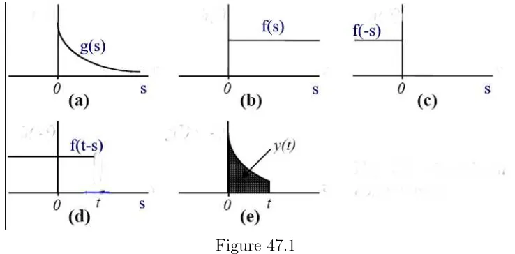
Graphical Interpretation of Convolution Operation For the convolution
(f∗g)(t) =
Z t
0
f(t−s)g(s)ds
we perform the following:
Step 1. Given the graphs of f(s) and g(s).(Figure 47.1(a) and (b)) Step 2. Time reverse f(−s).(See Figure 47.1(c))
Step 3. Shiftf(−s) right by an amounttto getf(t−s).(See Figure 47.1(d)) Step 4. Determine the product f(t−s)g(s). (See Figure 47.1(e))
Step 5. Determine the area under the graph off(t−s)g(s) between 0 and t.
(See Figure 47.1(e))
Figure 47.1
Theorem 47.1
Letf(t), g(t), andk(t) be three piecewise continuous scalar functions defined for t≥0 and c1 and c2 are arbitrary constants. Then
(i) f∗g =g∗f (Commutative Law)
(ii) (f ∗g)∗k=f ∗(g∗k) (Associative Law)
(iii) f ∗(c1g+c2k) = c1f∗g+c2f ∗k (Distributive Law) Proof.
(i) Using the change of variables τ =t−s we find
(f ∗g)(t) = R0tf(t−s)g(s)ds
= −R0
t f(τ)g(t−τ)dτ
= R0tg(t−τ)f(τ)dτ = (g∗f)(t) (ii) By definition, we have
[(f ∗g)∗k)](t) = R0t(f ∗g)(t−u)k(u)du
= Rt
0
h Rt−u
0 f(t−u−w)g(w)k(u)dw
i
du
For the integral in the bracket, make change of variable w=s−u. We have
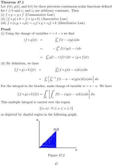
[(f ∗g)∗k)](t) =
Z t
0
Z t
u
f(t−s)g(s−u)k(u)ds
du.
This multiple integral is carried over the region
{(s, u) : 0≤u≤s≤t} as depicted by shaded region in the following graph.
Changing the order of integration, we have
[(f ∗g)∗k)](t) = R0tR0sf(t−s)g(s−u)k(u)duds
= Rt
0 f(t−s)(g∗k)(s)ds
= [f∗(g∗k)](t)
(iii) We have
(f ∗(c1g+c2k))(t) =
Rt
0 f(t−s)(c1g(s) +c2k(s))ds
= c1
Rt
0f(t−s)g(s)ds+c2
Rt
0 f(t−s)k(s)ds
= c1(f∗g)(t) +c2(f ∗k)(t)
Example 47.3
Express the solution to the initial value problem y0 +αy =g(t), y(0) = y0
in terms of a convolution integral.
Solution.
Solving this initial value problem by the method of integrating factor we find
y(t) =e−αty0+
Z t
0
e−α(t−s)g(s)ds=e−αty0+e−αt∗g(t)
Example 47.4
Iff(t) is anm×n matrix function and g(t) is ann×pmatrix function then we define
(f ∗g)(t) =
Z t
0
f(t−s)g(s)ds, t≥0.
Express the solution to the initial value problem y0 =Ay+g(t), y(0) =y0
in terms of a convolution integral.
Solution.
The unique solution is given by
y(t) = etAy0+
Z t
0
eA(t−s)g(s)ds =etAy0+etA∗g(t)
Theorem 47.2
If f(t) and g(t) are piecewise continuous for t ≥0, and of exponential order at infinity then
L[(f∗g)(t)] = L[f(t)]L[g(t)] =F(s)G(s).
Thus, (f ∗g)(t) =L−1[F(s)G(s)].
Proof.
First we show that f ∗g has a Laplace transform. From the hypotheses we have that |f(t)| ≤ M1ea1t for t ≥ C1 and |g(t)| ≤ M2ea2t for t ≥ C2. Let M =M1M2 and C =C1+C2. Then for t≥C we have
|(f ∗g)(t)| =
Rt
0 f(t−s)g(s)ds
≤
Rt
0 |f(t−s)||g(s)|ds
≤ M1M2
Rt
0 e
a1(t−s)ea2sds
=
M tea1t, a
1 =a2 Meaa2t−ea1t
2−a1 , a1 6=a2
This shows that f ∗g is of exponential order at infinity. Since f and g are piecewise continuous, the first fundamental theorem of calculus implies that
f ∗g is also piecewise continuous. Hence, f∗g has a Laplace transform. Next, we have
L[(f∗g)(t)] = R∞
0 e
−stRt
0 f(t−τ)g(τ)dτ
dt
= Rt∞=0Rτt=0e−stf(t−τ)g(τ)dτ dt
Note that the region of integration is an infinite triangular region and the integration is done vertically in that region. Integration horizontally we find
L[(f∗g)(t)] =
Z ∞
τ=0
Z ∞
t=τ
e−stf(t−τ)g(τ)dtdτ.
We next introduce the change of variablesβ =t−τ. The region of integration becomes τ ≥0, t ≥0. In this case, we have
L[(f ∗g)(t)] = Rτ∞=0Rβ∞=0e−s(β+τ)f(β)g(τ)dτ dβ
= Rτ∞=0e−sτg(τ)dτR∞
β=0e
−sβf(β)dβ
Example 47.5
Use the convolution theorem to find the inverse Laplace transform of
H(s) = 1 (s2+a2)2.
Solution. Note that
H(s) =
1
s2+a2
1
s2+a2
.
So, in this case we have,F(s) = G(s) = s2+1a2 so thatf(t) =g(t) =
1
asin (at).
Thus,
(f ∗g)(t) = 1
a2
Z t
0
sin (at−as) sin (as)ds= 1
2a3(sin (at)−atcos (at))
Convolution integrals are useful in solving initial value problems with forcing functions.
Example 47.6
Solve the initial value problem
4y00+y=g(t), y(0) = 3, y0(0) =−7 Solution.
Take the Laplace transform of all the terms and plug in the initial conditions to obtain
4(s2Y(s)−3s+ 7) +Y(s) =G(s) or
(4s2+ 1)Y(s)−12s+ 28 =G(s).
Solving for Y(s) we find
Y(s) = 12s−28
4(s2+1 4)
+ G(s)
4(s2+1 4)
= 3s
s2+((1 2)
2 −7
(1 2)
2
s2+(1 2)
2 +
1 4G(s)
(1 2)
2
s2+(1 2)
2
Hence,
y(t) = 3 cos
t
2
−7 sin
t 2 +1 2 Z t 0
sins 2
g(t−s)ds.
Practice Problems
Problem 47.1
Consider the functions f(t) =g(t) =h(t), t≥0 whereh(t) is the Heaviside unit step function. Compute f ∗g in two different ways.
(a) By directly evaluating the integral.
(b) By computing L−1[F(s)G(s)] where F(s) =L[f(t)] and G(s) = L[g(t)].
Problem 47.2
Consider the functions f(t) = et and g(t) = e−2t, t ≥ 0. Compute f ∗g in
two different ways.
(a) By directly evaluating the integral.
(b) By computing L−1[F(s)G(s)] where F(s) =L[f(t)] and G(s) = L[g(t)].
Problem 47.3
Consider the functions f(t) = sint and g(t) = cost, t≥0. Computef∗g in two different ways.
(a) By directly evaluating the integral.
(b) By computing L−1[F(s)G(s)] where F(s) =L[f(t)] and G(s) = L[g(t)].
Problem 47.4
Use Laplace transform to comput the convolution P∗y, where |bf P(t) =
h(t) et
0 t
and y(t) =
h(t)
e−t
.
Problem 47.5
Compute and graph f ∗g wheref(t) = h(t) and g(t) =t[h(t)−h(t−2)].
Problem 47.6
Compute and graph f∗g wheref(t) =h(t)−h(t−1) and g(t) =h(t−1)− 2h(t−2)].
Problem 47.7 Compute t∗t∗t.
Problem 47.8
Compute h(t)∗e−t∗e−2t.
Problem 47.10
Suppose it is known that
n f unctions
z }| {
h(t)∗h(t)∗ · · · ∗h(t) = Ct8. Determine the con-stants C and the poisitive integer n.
Problem 47.11
Use Laplace transform to solve for y(t) :
Z t
0
sin (t−λ)y(λ)dλ=t2.
Problem 47.12
Use Laplace transform to solve for y(t) :
y(t)−
Z t
0
e(t−λ)y(λ)dλ=t.
Problem 47.13
Use Laplace transform to solve for y(t) :
t∗y(t) = t2(1−e−t).
Problem 47.14
Use Laplace transform to solve for y(t) :
y0 =h(t)∗y, y(0) =
1 2
.
Problem 47.15
Solve the following initial value problem.
y0−y=
Z t
0