RIMBAY – a multi-approximation 3D ice-dynamics model for comprehensive applications: model description and examples

(1)

Geosci. Model Dev., 7, 1–21, 2014 www.geosci-model-dev.net/7/1/2014/ doi:10.5194/gmd-7-1-2014

Geoscientific

Model Development

Open Access

R

IMBAY

– a multi-approximation 3D ice-dynamics model for

comprehensive applications: model description and examples

M. Thoma1,2, K. Grosfeld1, D. Barbi1, J. Determann1, S. Goeller1, C. Mayer2, and F. Pattyn3

1_{Alfred Wegener Institute Helmholtz Center for Polar and Marine Research, Bussestrasse 24, 27570 Bremerhaven, Germany} 2_{Bavarian Academy of Sciences, Commission for Glaciology, Alfons-Goppel-Str. 11, 80539 Munich, Germany}

3_{Laboratoire de Glaciologie, Département des Sciences de la Terre et de l’Environnement (DSTE),} Université Libre de Bruxelles (ULB), CP 160/03, Avenue F.D. Roosevelt, 1050 Bruxelles, Belgium Correspondence to: M. Thoma ([email protected])

Received: 30 May 2013 – Published in Geosci. Model Dev. Discuss.: 19 June 2013 Revised: 28 November 2013 – Accepted: 1 December 2013 – Published: 7 January 2014

Abstract. Glaciers and ice caps exhibit currently the largest cryospheric contributions to sea level rise. Modelling the dy-namics and mass balance of the major ice sheets is therefore an important issue to investigate the current state and the fu-ture response of the cryosphere in response to changing envi-ronmental conditions, namely global warming. This requires a powerful, easy-to-use, versatile multi-approximation ice dynamics model. Based on the well-known and established ice sheet model of Pattyn (2003) we develop the modular multi-approximation thermomechanic ice model RIMBAY, in which we improve the original version in several aspects like a shallow ice–shallow shelf coupler and a full 3D-grounding-line migration scheme based on Schoof’s (2007) heuristic an-alytical approach. We summarise the full Stokes equations and several approximations implemented within this model and we describe the different numerical discretisations. The results are cross-validated against previous publications deal-ing with ice modelldeal-ing, and some additional artificial set-ups demonstrate the robustness of the different solvers and their internal coupling. RIMBAYis designed for an easy adaption to new scientific issues. Hence, we demonstrate in very dif-ferent set-ups the applicability and functionality of RIMBAY in Earth system science in general and ice modelling in par-ticular.

1 Introduction

According to the Fourth Assessment Report (AR4) of the Intergovernmental Panel on Climate Change (IPCC) (IPCC, 2007) it is unequivocal, that Earth’s climate is warming since about 1850. This trend has been observed e.g. in rising air and ocean temperatures, in increased snow and ice melting, and in a rising sea level. According to more recent publica-tions (e.g. Church et al., 2011; Rahmstorf et al., 2012) the trends estimated even for the worst scenarios of the AR4 are already reached or surpassed. Therefore, the imminent climate change will have profound impact on society (e.g. Hanson et al., 2011).

(2)

2 M. Thoma et al.: Description of the ice flow model RIMBAY

2 M. Thoma et al.: Description of the ice flow model RIMBAY

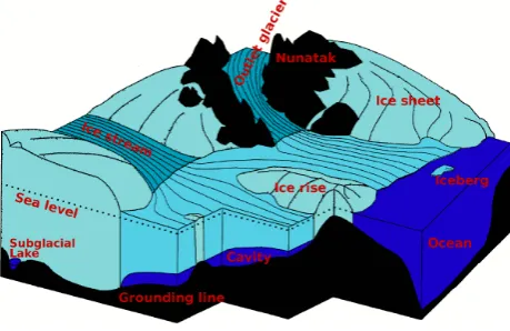
Fig. 1.Sketch illustrating several aspects/components to be

consid-ered in ice sheet modelling (adapted after Sandhäger, 2000).

oped since 2009. Although the underlying Higher Order

70

Model (HOM) and Full Stokes (FS)-physics remained ba-sically unchanged, a Shallow Shelf Approximation (SSA) solver has been added to calculate the horizontally averaged velocities of ice streams and ice shelves. Additionally, the numerical solver implementation, the discretisation, the

cou-75

pling between different solvers and the user interface have been improved in many aspects since it diverted from the original model. Keeping in mind that ice models have to deal with many different geophysical settings and boundary conditions, it is challenging to design a computer code which

80

is able to fulfil these needs for a large variety of users and ap-plications. RIMBAYhas been designed to be easy applicable to new scenarios, easy to extend and with clear interfaces to couple it with existing codes.

This paper is structured as follows: First, we clarify in

85

section 2 the sometimes imprecise usage of the termmodel, before we present in section 3 the mathematical equations and several approximations founding the mathematical back-ground of RIMBAY. Thereafter, we describe the numerical finite-difference implementation of these equations and how

90

they can be solved with existing numerical solvers for lin-ear differential equations in section 4. Some more details about the code–implementation are given in section 5, before we present some idealised example–applications of RIMBAY, with a main focus on cross-validation with previously

pub-95

lished ice-model results and an example of internal code-coupling in section 6. Finally, we demonstrate in section 7 the wide spectrum of applications RIMBAYis already used for by several users.

2 Multi-approximation ice sheet/shelf model RIMBAY

100

The termmodelis used in several ways in Earth system sci-ence, which can be sometimes confusing. Therfore, we first define what we understand asmodel, or to be more precise between which types ofmodelwe distinguish:

– Equations form themathematical modeldescribing the

105

fundamental relationship between the relevant values of interest (e.g., velocity, temperature, and viscosity). In our context, these equations are mostly coupled differ-ential equations which can not be solved analytically.

– These equations are solved with a computer, which

re-110

quires a discretisation of the equations. This can be done in several distinct ways, depending on the demand of accuracy, stability, convergence properties, and re-sources (memory usage and computational coast). We refer to this as thenumerical model.

115

– This numerical model has to be translated into a com-puter language (mostly a high-level programming lan-guage like Matlab, Fortran, C, or C++). It is common sense to refer to this computer program as model, too. We use the expressioncodeor the implementation to

120

specify the lines forming this (sometimes compiled bi-nary) program.

– Finally, the code is applied to answer a specific scien-tific question (e.g. the contribution to sea level rise) of a specific domain (e.g., whole Antarctica or a subregion

125

like the area of the Pine Island Glacier), or to study pro-cesses (e.g. the impact of basal water on ice dynamics) and the sensitivity to parameters or boundary conditions (e.g. geothermal heat flux, bedrock topography or ice thickness distribution). These applications of a

com-130

puter program are often calledmodel, too.We refer to these applications asexperimentsorscenarios.

In general, we use the term RIMBAYfor the implementation of the discretised equation, and therefore the compiled bi-nary code, which includes not only the mathematical model,

135

but also a sophisticated command-line interpreter and input-output interfaces for an easy usage. RIMBAYis distributed with a suit of example– and reference–scenarios and several additional programs (mainly based on the bash-script lan-guage) providing several options to visualize the computed

140

results with the Generic Mapping Tools (GMT, Wessel and Smith, 1998; Wessel et al., 2013). In the following sections, we elaborate on these different model types and how they are used in RIMBAY.

3 Mathematical model

145

The mathematical field equations are based upon the conser-vation of mass, momentum, and energy

∂ρ

∂t +∇ ·(ρv) = 0 (1) ρdv

dt =∇ ·τ+ρg (2) ρcd(θ)

dt =∇(κ∇θ) +Qi (3) with the (constant) density ρ, the velocity vector v = (vx, vy, vz) = (u, v, w), the gravitational accelerationg =

Fig. 1. Sketch illustrating several aspects/components to be

consid-ered in ice sheet modelling (adapted after Sandhäger, 2000).

iceberg calving. Therefore, a numerical model has to deal with many different aspects of an ice sheet (and ice shelf) to represent it’s complex dynamic behaviour adequately and to improve future projections or hindcasts for palaeoclimatol-ogy.

During the last years great efforts have been undertaken to improve existing ice models and to incorporate them into coupled climate models (e.g. Rutt et al., 2009; Gillet-Chaulet et al., 2012; Levermann et al., 2012). Here, we present the Revised Ice Model Based on frAnk pattYn, the multi-approximation ice sheet/ice shelf model RIMBAY. This model is originally based on the higher-order numeri-cal ice-flow model of Pattyn (2003), which has been tested and applied to many scenarios (e.g. Pattyn, 2002; Pattyn et al., 2004; Pattyn, 2008, 2010). RIMBAY itself has been developed since 2009. Although the underlying higher order model (HOM) and full Stokes (FS)-physics remained basi-cally unchanged, a shallow shelf approximation (SSA) solver has been added to calculate the horizontally averaged veloc-ities of ice streams and ice shelves. Additionally, the numer-ical solver implementation, the discretisation, the coupling between different solvers and the user interface have been improved in many aspects since it diverted from the orig-inal model. Keeping in mind that ice models have to deal with many different geophysical settings and boundary con-ditions, it is challenging to design a computer code which is able to fulfil these needs for a large variety of users and ap-plications. RIMBAYhas been designed to be easy applicable to new scenarios, easy to extend and with clear interfaces to couple it with existing codes.

This paper is structured as follows: first, we clarify in Sect. 2 the sometimes imprecise usage of the term model, before we present in Sect. 3 the mathematical equations and several approximations founding the mathematical back-ground of RIMBAY. Thereafter, we describe the numerical finite-difference implementation of these equations and how they can be solved with existing numerical solvers for linear

differential equations in Sect. 4. Some more details about the code implementation are given in Sect. 5, before we present some idealised example applications of RIMBAY, with a main focus on cross-validation with previously pub-lished ice-model results and an example of internal code cou-pling in Sect. 6. Finally, we demonstrate in Sect. 7 the wide spectrum of applications RIMBAYis already used for by sev-eral users.

2 Multi-approximation ice sheet/shelf model RIMBAY

The term model is used in several ways in Earth system sci-ence, which can be sometimes confusing. Therefore, we first define what we understand as model and, to be more precise, between which types of models we distinguish.

– Equations form the mathematical model describing the fundamental relationship between the relevant values of interest (e.g. velocity, temperature, and viscosity). In our context, these equations are mostly coupled dif-ferential equations which can not be solved analyti-cally.

– These equations are solved with a computer, which requires a discretisation of the equations. This can be done in several distinct ways, depending on the demand of accuracy, stability, convergence proper-ties, and resources (memory usage and computational coast). We refer to this as the numerical model. – This numerical model has to be translated into a

com-puter language (mostly a high-level programming lan-guage like Matlab, Fortran, C, or C++). It is common sense to refer to this computer program as model, too. We use the expression code or the implementation to specify the lines forming this (sometimes compiled bi-nary) program.

– Finally, the code is applied to answer a specific scien-tific question (e.g. the contribution to sea level rise) of a specific domain (e.g. whole Antarctica or a subregion like the area of the Pine Island Glacier), or to study processes (e.g. the impact of basal water on ice dy-namics) and the sensitivity to parameters or boundary conditions (e.g. geothermal heat flux, bedrock topog-raphy or ice thickness distribution). These applications of a computer program are often called model, too. We refer to these applications as experiments or scenarios. In general, we use the term RIMBAYfor the implementation of the discretised equation, and therefore the compiled bi-nary code, which includes not only the mathematical model, but also a sophisticated command-line interpreter and input-output interfaces for an easy usage. RIMBAY is distributed with a suit of example – and reference – scenarios and several

(3)

M. Thoma et al.: Description of the ice flow model RIMBAY 3 additional programs (mainly based on the bash-script

lan-guage) providing several options to visualise the computed results with the generic mapping tools (GMT) (GMT, Wessel and Smith, 1998; Wessel et al., 2013). In the following sec-tions, we elaborate on these different model types and how they are used in RIMBAY.

3 Mathematical model

The mathematical field equations are based upon the conser-vation of mass, momentum, and energy:

∂ρ

∂t + ∇ ·(ρv)=0, (1)

ρdv

dt = ∇ ·τ+ρg, (2)

ρcdθ

dt = ∇(κ∇θ )+Qi, (3)

with the (constant) density ρ, the velocity vector v= (vx, vy, vz)=(u, v, w), the gravitational acceleration g=

(0,0,−g), the two dimensional stress tensorτ, the (poten-tial) temperatureθ, the heat capacityc, the thermal conduc-tivityκ, and the internal frictional heatingQi. In the

follow-ing we consider Cartesian coordinates, with the vertical co-ordinatez upwards and neglect acceleration. In case of an incompressible fluid with a constant density the continuity equation (conservation of mass) follows as

∇ ·v=∂u

∂x+ ∂v ∂y+

∂w

∂z =0. (4)

The stress tensorτ is split into a deviatoric partτ0 _{and an} isotropic pressure, which is defined as the negative trace of the stress tensor:

τ=τ0+1

3 τxx+τyy+τzz

1

=τ0−p1,

(5) where 1 symbolises the identity matrix.

3.1 Equation of motion

Because velocities in ice sheet/shelf modelling are rather small, acceleration can be ignored and the momentum equa-tion can be written as

∂τ_xx0

∂x +

∂τ_xy0

∂y +

∂τ_xz0

∂z −

∂p ∂x =0, ∂τ_yx0

∂x +

∂τ_yy0

∂y +

∂τ_yz0

∂z −

∂p ∂y =0, ∂τ_zx0

∂x +

∂τ_zy0

∂y +

∂τ_zz0

∂z −

∂p

∂z =ρg. (6)

According to Paterson (1994), the constitutive equation for polycrystalline ice links the deviatoric stresses to the strain rates,

τ0=2η˙=2η





˙

xx ˙xy˙xz ˙

yx ˙yy˙yz ˙

zx ˙zy ˙zz





=2η



   

∂u ∂x

1 2

∂u ∂y+

∂v ∂x

1 2

∂u ∂z+

∂w ∂x

1 2

∂u

∂y +

∂v ∂x

∂v ∂y

1 2

∂v ∂z+

∂w ∂y

1 2

∂u ∂z+

∂w ∂x

1 2

∂v ∂z+

∂w ∂y

∂w ∂z



   

, (7)

applying the effective viscosityη, which can be described by the Glen-type flow law (e.g. Cuffey and Paterson, 2010):

˙

=A(θ )ˆ τ0n, or τ0=2η˙ with

η:=1

2A(

ˆ

θ )−1n˙(1−nn)_, ₍₈₎

withn=3, the pressure-corrected ice temperature θˆ=θ+ αp, with a constantα=9.8×10−4K Pa−1(Greve and Blat-ter, 2009), and the effective strain rate (valid for incompress-ibility as˙xx+ ˙yy+ ˙zz=0 follows from Eq. 4)

˙

=

q

˙ 2

xx+ ˙yy2 + ˙xx˙yy+ ˙xy2 + ˙2xz+ ˙yz2. (9)

The temperature dependent rate factorA(θ )ˆ is parameterised according to the Arrhenius relationship after Hooke (1981) or Paterson and Budd (1982). Combining Eq. (6) and Eq. (7) we get the so-called full Stokes (FS) equations for ice modelling:

∂ ∂x

2η∂u

∂x

+ ∂

∂y

η∂u ∂y +η

∂v ∂x

+ ∂

∂z

η∂u ∂z+η

∂w ∂x

−∂p

∂x=0, ∂

∂x

η∂u ∂y+η

∂v

∂x

+ ∂

∂y

2η∂v

∂y

+ ∂

∂z

η∂v ∂z+η

∂w ∂y

−∂p

∂y =0, ∂

∂x

η∂u ∂z+η

∂w ∂x

+ ∂

∂y

η∂v ∂z+η

∂w ∂y

+ ∂

∂z

2η∂w

∂z

−∂p

∂z =ρg. (10)

Rearranging Eq. (5) leads to

p= −τ_xx0 −τ_yy0 −τzz

= −2η

_∂u

∂x+ ∂v ∂y

−τzz, (11)

with an expression for the vertical normal stressτzzobtained

(4)

surfaceSto the heightz(Van der Veen and Whillans, 1989; Pattyn, 2008):

τzz= −ρg (S−z)+

∂ ∂x

S

Z

z

τ_xz0 dz0+ ∂ ∂y

S

Z

z

τ_yz0 dz0

| {z }

Rzz

. (12)

Here, the first term in Eq. (12) describes the hydrostatic part andRzzthe resistive part, sometimes also referred to as

ver-tical resistive longitudinal stress.

Depending on the scientific issue, several approximations of Eq. (10) might be reasonable, which are described in the following subsection.

3.2 Higher-order approximation

The HOM approximation of Pattyn (2003) applies the hydro-static approximation, by neglecting the resistive stressRzzin

Eqs. (10)–(12) for the vertical velocity and the vertical nmal stress. These are only relevant (but still almost two or-ders of magnitude below the other normal stress and shear stress components, Pattyn, 2000) where the ice flow regime changes, as in the vicinity of ice margins or ice divides. Ad-ditionally, ignoring the horizontal derivatives of the vertical velocity in Eq. (10), leads to

∂ ∂x

2η∂u

∂x

+ ∂

∂y

η∂u ∂y+η

∂v ∂x

+ ∂

∂z

η∂u ∂z

−∂p

∂x=0, ∂

∂x

η∂u ∂y+η

∂v ∂x

+ ∂

∂y

2η∂v

∂y

+ ∂

∂z

η∂v ∂z

−∂p

∂y =0, ∂

∂z

2η∂w

∂z

−∂p

∂z=ρg. (13)

Applying Eqs. (11) and (12) we obtain ∂

∂x

2η

2∂u

∂x+ ∂v ∂y

+ ∂

∂y

η

∂u ∂y +

∂v ∂x

+ ∂

∂z

η∂u ∂z

=ρg∂S ∂x, ∂

∂y

2η

2∂v

∂y+ ∂u ∂x

+ ∂

∂x

η

∂u ∂y+

∂v ∂x

+ ∂

∂z

η∂v ∂z

=ρg∂S

∂y, (14) for the horizontal velocities. The vertical velocity at depthz

can be derived by integrating the continuity equation Eq. (4) from the baseBvertically:

w(z)=w(B)− z

Z

B

_∂u

∂x+ ∂v ∂y

dz0. (15)

3.3 Shallow shelf or shelfy stream approximation

A second common approximation is the shallow shelf ap-proximation or shelfy stream apap-proximation (SSA). This assumes that the horizontal velocity is depth-independent (∂u_∂z =∂v

∂z =0), which is the case for ice shelf regions and fast

flowing ice streams decoupled from the ground. Integrating Eq. (14) through the ice from the baseBto the surfaceS, and definingUandV as the vertically integrated velocities leads to (e.g. Morland, 1987; MacAyeal, 1989; Pattyn, 2010)

∂ ∂x

2H η

2∂U

∂x +

∂V ∂y

+ ∂

∂y

H η

_∂U

∂y +

∂V ∂x

−τbx=ρgH

∂S ∂x, ∂

∂y

2H η

2∂V

∂y +

∂U ∂x

+ ∂

∂x

H η

_∂U

∂y +

∂V ∂x

−τby=ρgH

∂S

∂y, (16)

where the basal shear stressτbiretards the otherwise

unham-pered flow on bedrock till. It can be expressed in terms of the basal friction parameterβ2 and the horizontal velocity:

τbi =β2Vi. A thorough derivation of Eq.16 can be found in

Greve and Blatter (2009). Both, the shelfy stream approxi-mation and the shallow shelf approxiapproxi-mation are expressed by Eq. (16). The only difference is, that for an ice shelf or above a subglacial lake β2 is zero, while it might reach several thousand Pa a m−1for a slippery bedrock, which especially applies to basal lubricated areas. As a rule of thumb above dry bedrock a value of β2=25 000 Pa a m−1 would corre-spond to a typical frictional stress of about 100 kPa (Pater-son, 1994) if a velocity of about 4 m a−1is assumed (Thoma et al., 2012). Finally, because of the lacking vertical shear stresses Eq. (9) reduces to

˙ =q˙2

xx+ ˙yy2 + ˙xx˙yy+ ˙xy2 . (17)

3.4 Shallow ice approximation

The most rigid approximation is the shallow ice approxima-tion (SIA, which is a reasonable simplificaapproxima-tion for large ice bodies, when the horizontal length scale is much larger than the ice thickness (e.g. Hutter, 1983). Assuming that the hori-zontal derivation of the vertical velocity is much smaller than the vertical derivation of the horizontal velocity (∂w_∂x ∂u

∂z)

and applying the hydrostatic approximation (which reduces the vertical momentum balance to the hydrostatic term) we derive

∂ ∂z

η∂u ∂z

−∂p

∂x=0, ∂

∂z

η∂v ∂z

−∂p

∂y =0,

−∂p

∂z =ρg. (18)

(5)

M. Thoma et al.: Description of the ice flow model RIMBAY 5 Basically, this approximation decouples the horizontal

veloc-ities, allowing local solutions for the velocity field, instead of a much more complex and time-consuming implicit solver. The numerical resources of this SIA are so low (compared to any other approximations) that it is still widely used (and useful) for many applications.

3.5 Boundary conditions

Several boundary conditions have to be formulated to solve the different approximations of the equation of motion.

1. We apply a stress-free surface boundary condition:

τs·ns=0, (19)

with the normal vectornsorthogonal to the surface. 2. For the horizontal velocities at the ice base, we apply

either

– a no-slip condition for the tangential velocities (vk=vb−nb(vb·nb)=0).

– a Weertman-type sliding law (e.g. Paterson, 1994; Cuffey and Paterson, 2010), linking the sliding velocity with the basal shear stress: τb=β2vb =C|vb|m−1vb or

vb=

1

β2τb =C

−1

m|τb|

1

m−1_τ_b_, ₍₂₀₎

with the basal tangential stress componentτb=

τ·nband the normal vectornborthogonal to the

ice base, the basal friction coefficientC, and the basal friction exponentm.

The basal drag is defined as the sum of all basal resistive forces (Van der Veen and Whillans, 1989; Pattyn, 2003):

τbx=τxz0 −

2τ_xx0 +τ_yy0 +Rzz

∂B

∂x −τ 0

xy

∂B ∂y ,

τby=τyz0 −

2τ_yy0 +τ_xx0 +Rzz

∂B

∂y −τ 0

xy

∂B ∂x

, (21)

withτ_ij0 =τ_ij0(B). In case of the SIA these equa-tions simplify to

τbx= −ρgH

∂S

∂x, τby= −ρgH

∂S

∂y. (22)

– or a stress free base when a substantial amount of water is present, like in the case of subglacial lakes and ice shelves; this impliesβ2=0. 3. For the vertical velocity at the base, we apply a

kine-matic boundary condition:

wB=

∂B ∂t +u

∂B ∂x +v

∂B

∂y − ˙mB, (23)

with the basal melt ratem˙B.

4. At lateral boundaries of the model domain, we apply either

– zero ice thickness (H=0),

– Dirichlet boundary conditions with fixed veloci-ties. The no-slip condition (u=0), which would imply frozen ice at nunataks, is a special case of this.

– A Neumann free-slip boundary condition:

∇vi·ni=0,

[∇(v−(v·n⊥)n⊥)]n⊥=0, (24) at ice-nunatak edges, with the unit vectorn⊥ or-thogonal to the edge, or

– a (dynamic) Neumann boundary condition for an ice shelf–ocean interface (e.g. Greve and Blatter, 2009; Joughin et al., 2009; Pattyn, 2010), 2µH

2∂U

∂x +

∂V ∂y

nx

+µH

_∂U

∂y +

∂V

∂x

ny=

ρgH Snx

2 ,

2µH

2∂V

∂y +

∂U ∂x

ny

+µH

_∂V

∂x +

∂U ∂y

nx=

ρgH Sny

2 , (25)

with the outward-pointing unit vector (nx, ny),

which is perpendicular to the (vertical) ice shelf front.

– or periodic boundary conditions.

These equations are converted in terrain followingσ coor-dinates by applying

σ=S−z

H , (26)

with the ice thicknessHand the surface heightS. This coor-dinate transformation leads to additional metric terms in the equations, which are described in detail in Pattyn (2003) or Greve and Blatter (2009). The advantage is, that the verti-cal coordinate ranges fromσ =0 at the surface toσ=1 at the ice base, independent of the local ice thickness and the bedrock elevation.

3.6 Temperature calculation

Assuming a constant thermal conductivityκ, the temperature evolution (Eq. 3) can be divided into an advective, a diffusive and a source term:

ρc





∂θ

∂t + v| {z }· ∇θ Advection



= κ∇2θ | {z } Diffusion

+ Qi

|{z} Internal Sources

(6)

Neglecting horizontal diffusion and assuming that the in-ternal heat source results mainly from the ice deforma-tion (Paterson, 1994) we obtain with the effective deviatoric stressτ0(defined similar to the effective strain rate in Eq. 9) andQi=2τ˙ 0=4η˙2

∂θ ∂t =

κ ρc

∂2θ ∂z2−u

∂θ ∂x−v

∂θ ∂y−w

∂θ ∂z+

4η˙2

ρc . (28)

The boundary conditions applied to solve this thermody-namic equation are

– the mean air temperature at the surface of the ice body,

– a Dirichlet boundary condition according to the pres-sure melting point of ice (e.g. Paterson, 1994), θ= −8.7×10−4K m−1H, at the ice base when the ice is floating (like above subglacial lakes and for ice shelves), and

– a Neumann boundary condition at the base b for grounded ice:

∂θb

∂z = −

G+τ_b0|vb|

κ , (29)

with the basal stressτ_b0=qτ_bx2 +τ_by2 and the geother-mal heat fluxG.

3.7 Ice sheet evolution

Integration of Eq. (1) from the baseB to the surfaceSleads to an equation for the ice evolution. Defining the ice thick-nessH=S−B, accounting for melting or accumulation at the surface and/or base and assuming a constant ice density

ρwe get

∂ ∂t

S

Z

B

ρ dz+ ∇ · S

Z

B

(ρvi) dz=ρm,˙ (30)

∂H

∂t = −

_{∂ UH}

∂x +

∂ VH ∂y

+ ˙m, (31)

with the mass balance (in m a−1) is defined as

˙

m= m˙ac

|{z} Accumulation

− m˙ab

|{z} Ablation

− m˙B

|{z} Basal melting

. (32)

Basal freezing can be implemented by negative basal melt-ing.

4 Numerical model

4.1 Linear and non-linear solvers

The coupled pair of equations for the horizontal velocity field for the FS, HOM, and SSA equations (Eqs. 10, 14, 16)

depend on the strain-rate dependent viscosity (Eq. 8), result-ing in a non-linear problem. In the full Stokes case, the hor-izontal velocities depend also on the vertical velocity. How-ever, these problems can be solved iteratively as indicated in Fig. 2.

In the full Stokes case, the vertical velocity w can be estimated from the continuity Eq. (4), imposing kinematic boundary condition at the lower ice surface (including melt rates).

According to Pattyn (2003), it is sufficient to solve the system of linear equations foruandvsuccessively, instead of solving both equations at once. In general, we iteratively solve

Anm(x_ijl )·xml+1=bn(x_ijl ), (33)

wherelis the iteration,Anmcontains the coefficients of the

left-hand side of the relevant equation to solve, whilebn is

the forcing term on the right-hand side of the equation. The placeholderxmsymbolises the horizontal velocitiesuijorvij

(Eqs. 10, 14, or 16), the potential temperatureθij (Eq. 28),

or the ice thickness Hij (Eq. 31), respectively. The indices

nandmsymbolise the consecutively numbered grid nodes from(j=1, i=1)to(j=Xmax, i=Ymax)1.

Two methods to solve the linear system of Eq. (33) are available within RIMBAY: first, the fast and efficient biconju-gate gradient method with a Jacobian preconditioner (linbcg) from the numerical recipes (NR) (Press et al., 2007); second, the Library of Iterative Solvers (LIS) from Nishida (2010).

The Library of Iterative Solvers (LIS) provides a bunch of preconditioners and solvers, including the recommend-able generalised minimal residual (gmres) method, which can also be applied to solve non-symmetric matrices. For both methods the effective compressed row storage (CRS) sparse matrix method is used as a default to store the ele-ments of the matrixAnm. However, for the LIS, the modified

sparse row (MSR) format is implemented, too. Comparisons with respect to the calculated velocities have shown

– the differences for the two storage formats (CRS vs. MSR) are negligible,

– the differences between the linbcg solver from Press et al. (2007) and the very same preconditioner/solver combination from the Library of Iterative Solvers are negligible, but the solver of Press et al. (2007) needs less computational resources.

– if specific preconditioner–solver combinations con-verge, the difference between different combinations are negligible.

Summarised, if a solution of the linear system can be com-puted with a reasonable accuracy, the results can be trusted. 1_{Note, that for historical reasons (originating from Pattyn, 2003,}

2008) the order ofiandj is swapped within RIMBAY, compared with the intuitive usage.

(7)

M. Thoma et al.: Description of the ice flow model RIMBAY 7

Temperature IeEvolution VertialVeloity HorizontalVeloity

BasalConditions SIA η (u, v)

SSA Hη (u, v)

HOM FS

η w

Rzz

(u, v)

Fig. 2.Sequence of iteratively solved variables within RIMBAY. In the SSA-case the product ofHηis calculated, instead of the viscos-ityη, only. The grayish highlighted variables are calculated only in the FS-case. (Within the main loop, the vertical velocity needs only to be calculated in the non FS-cases.)

get ∂ ∂t S Z B

ρ dz+∇ · S

Z

B

(ρvi)dz=ρm˙ (30)

∂H ∂t =−

_{∂ UH}

∂x + ∂ VH

∂y

+ ˙m (31) with the mass balance (in m/a) is defined as

˙

m= m˙ac

|{z}

Accumulation

− m˙ab

|{z}

Ablation

− m˙B

|{z}

Basal melting

(32)

Basal freezing can be implemented by negative basal

melt-205

ing.

4 Numerical model

4.1 Linear and non-linear solvers

The coupled pair of equations for the horizontal velocity field for the FS, HOM, and SSA equations (Eq. 10, Eq. 14,

210

and Eq. 16) depend on the strain-rate dependent viscosity (Eq. 8), resulting in a non-linear problem. In the full Stokes case, the horizontal velocities depend also on the vertical ve-locity. However, these problems can be solved iteratively as indicated by Fig. 2. In the full Stokes case, the vertical

ve-215

locitywcan be estimated from the continuity equation 4, im-posing kinematic boundary condition at the lower ice surface (including melt rates).

According to Pattyn (2003), it is sufficient to solve the sys-tem of linear equations foruandvsuccessively, instead of solving both equations at once. In general, we iteratively solve

Anm(xlij)·xml+1=bn(xlij) (33)

wherelis the iteration,Anmcontains the coefficients of the

left-hand side of the relevant equation to solve, whilebn is 220

the forcing term on the right-hand side of the equation. The placeholderxm symbolizes the horizontal velocities uij or

vij (Eq. 10, Eq. 14, or Eq. 16), the potential temperatureθij

(Eq. 28), or the ice thicknessHij(Eq. 31), respectively. The

indicesnandmsymbolize the consecutively numbered grid

225

nodes from(j= 1, i= 1)to(j=Xmax, i=Ymax)1.

Two methods to solve the linear system of Eq. 33 are avail-able within RIMBAY: First, the fast and efficient biconju-gate gradient method with a Jacobian preconditioner (linbcg) from theNumerical Recipes(NR) (Press et al., 2007), second

230

theLibrary of Iterative Solvers(LIS) from Nishida (2010). The Library of Iterative Solvers (LIS) provides a bunch of preconditioners and solvers, including the recommendable Generalized Minimal RESidual(gmres) method, which can also be applied to solve non-symmetric matrices. For both

235

methods the effectivecompressed row storage(CRS) sparse matrix method is used as a default to store the elements of the matrixAnm. However, for the LIS, themodified sparse

row(MSR) format is implemented, too. Comparisons with respect to the calculated velocities have shown

240

– the differences for the two storage formats (CRS vs. MSR) are negligible,

– the differences between the linbcg solver from Press et al. (2007) and the very same preconditioner/solver combination from theLibrary of Iterative Solvers are

245

negligible, but the solver of Press et al. (2007) needs less computational resources.

– ifspecific preconditioner–solver combination converge, the difference between different combinations are neg-ligible.

250

Summarised,if a solution of the linear system can be com-puted with a reasonable accuracy, the results can be trusted. In general, we suggest to start with the fasterlinbcg algo-rithm (from Press et al., 2007) and to switch to the gmres solver with a Jacobian or ILU (Incomplete LU

decomposi-255

tion) preconditioner if it should fail.

When solving the linearized equations for the horizon-tal velocity, the viscosity η might vary over a few orders of magnitude, which requires a sophisticated convergence scheme. Hence, a simple Picard iteration might fail.

There-260

fore, Pattyn (2003) extended this scheme by the unstable manifold correction(UMC), introduced by Hindmarsh and Payne (1996), which results in a proper convergence of the solution. In RIMBAYthe UMC is applied in the SSA, HOM, and FS solvers.

265

4.2 Discretisation

When equations are discretised, it is important to realize where exactly the individual variables are located. This is

1

Note, that for historical reasons (originating from Pattyn, 2003, 2008) the order ofiandj is swapped within RIMBAY, compared with the intuitive usage.

Fig. 2. Sequence of iteratively solved variables within RIMBAY. In

the SSA case the product ofH ηis calculated, instead of the viscos-ityη, only. The grayish highlighted variables are calculated only in the FS case. (Within the main loop, the vertical velocity needs only to be calculated in the non-FS cases.)

In general, we suggest to start with the faster linbcg algo-rithm (from Press et al., 2007) and to switch to the gmres solver with a Jacobian or ILU (Incomplete LU decomposi-tion) preconditioner if it should fail.

When solving the linearised equations for the horizontal velocity, the viscosityηmight vary over a few orders of mag-nitude, which requires a sophisticated convergence scheme. Hence, a simple Picard iteration might fail. Therefore, Pattyn (2003) extended this scheme by the unstable manifold cor-rection (UMC), introduced by Hindmarsh and Payne (1996), which results in a proper convergence of the solution. In RIMBAY the UMC is applied in the SSA, HOM, and FS solvers.

4.2 Discretisation

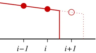
When equations are discretised, it is important to realise where exactly the individual variables are located. This is quite simply defined for the unstaggered Arakawa A-grid (e.g. Arakawa and Lamb, 1977; Purser and Leslie, 1988) where all variables are located in the very same grid posi-tion. However, sometimes a different approach has numeri-cal advantages. Besides the traditional (unstaggered) A-grid, the staggered Arakawa C-grid is optionally available in RIM-BAYfor the SIA and SSA solvers. On the Arakawa C-grid, the horizontal velocities are defined in between the thickness (and viscosity) nodes as illustrated in Fig. 3.

4.3 Ice Sheet evolution

As an example, we formulate the implemented discretisation of the ice sheet evolution (Eq. 31) explicitly for the two dif-ferent grids. Additionally, the detailed discretisation on the C-grid of the SSA equation of motion (Eq. 16) is given in Appendix B.

M. Thoma et al.: Description of the ice flow model RIMBAY 7

i−1,j−1 i,j−1 i+1,j−1 i−1,j i,j i+1,j i−1,j+1 i,j+1 i+1,j+1 i−1,j−1 i,j−1 i−1,j i,j i−1,j+1 i,j+1 i−1,j−1 i,j−1 i+1,j−1 i−1,j i,j i+1,j i,j i,j i,j

∆xH

∆xu

∆ y H ∆ y v i+1/2,j−1/2 i+1/2,j+1/2 i−1/2,j+1/2 ∆x*

∆

y

*

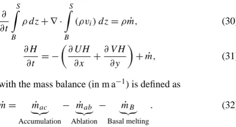
Fig. 3.Location of nodes on a C-Grid. The location ofH-,η-, and

θ-nodes are indicated by dots while the location of the horizontal velocities are indicated by arrows. The stars indicate certain inter-grid nodes used in the numerical implementation. The red color indicates corresponding nodes of the centrali,j–node and the color-coded increments (∆...) at the edges refer to the corresponding grid node distances.

quite simply defined for the unstaggered Arakawa A-Grid (e.g., Arakawa and Lamb, 1977; Purser and Leslie, 1988)

270

where all variables are located in the very same grid position. However, sometimes a different approach has numerical ad-vantages. Besides the traditional (unstaggered) A-Grid, the staggered Arakawa C-Grid is optionally available in RIM

-BAYfor the SIA-and SSA-solvers. On the Arakawa C-Grid,

275

the horizontal velocities are defined in between the thickness (and viscosity) nodes as illustrated in Fig. 3.

4.3 Ice Sheet evolution

As an example, we formulate the implemented discretisation of the ice sheet evolution (Eq. 31) explicitly for the two

dif-280

ferent grids. Additionally, the detailed discretisation on the C-grid of the SSA equation of motion (Eq. 16) is given in appendix B.

4.3.1 C-Grid

For the C-Grid, where the velocities are defined inbetween thickness nodes, the equation of the ice sheet evolution (Eq. 31) can be written as an implicit first order finite dif-ference equation as

1

2

3

4

5 y,v,i

x,u,j

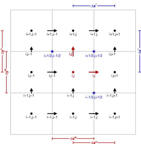
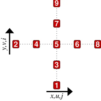
Fig. 4. Relative positions and numbering of nodes for the implicit first order finite difference formulation of the ice evolution (Eq.31).

Hi,jt+1+ ∆t

Ui,j(Hi,jt+1+1+H

t+1

i,j )−Ui,j−1(Hi,jt+1+H t+1

i,j−1)

2∆x

+∆t

Vi,j(Hit+1+1,j+H t+1

i,j )−Vi−1,j(Hi,jt+1+H t+1

i−1,j)

2∆y

=Hi,jt + ˙m∆t

(34)

Rearranging Eq. 34 with respect to the five discreteHt+1

-values, located and numbered as indicated by Fig.4, results in the following coefficients for the sparse matrixAnmof the

linear solver:

Cn1=−

∆t

2∆yVi−1,j Cn2=−

∆t

2∆xUi,j−1 Cn3=1 +

∆t

2

Ui,j−Ui,j−1

∆x +

Vi,j−Vi−1,j

∆y

Cn4= +

∆t

2∆xUi,j Cn5= +

∆t

2∆yVi,j bn=Hi,jt + ˙mi,j∆t

(35)

These coefficients represent the non-zero elements of each

285

single rownfor each ij-element of the matrixAnm, with

Cn3indicating the central node at(i,j) andbnindicates the

forcing term on the right-hand-side.

The coefficients derived in the last subsection are valid for the interior of the ice. Boundary conditions have to be

for-290

mulated at the edges of the ice sheet. Open boundariesfor grid cells adjacent to ocean or ice-free land are simply im-plicitly implemented by assumingH = 0at the respective grid cell.

If the ice adjoins a nunatak or a lateral end of the model

295

domain,closed boundaryconditions are applied. We define these by setting the velocity (and thus the flux) of ice over the edge of the specific grid cell, to zero. For example, closed boundaries at the eastern (Ui,j = 0) and southern (Vi−1,j =

0) edge would result inCn1 = Cn4 = 0andCn3 = 1 + 300 ∆t 2 _V i,j ∆y − Ui,j−1

∆x

in Eq. 35.

Fig. 3. Location of nodes on a C-grid. The location ofH,η, andθ

nodes are indicated by dots while the location of the horizontal ve-locities are indicated by arrows. The stars indicate certain inter-grid nodes used in the numerical implementation. The red colour indi-cates corresponding nodes of the centrali,j node and the colour-coded increments (1. . .) at the edges refer to the corresponding grid node distances.

4.3.1 C-grid

For the C-grid, where the velocities are defined in-between thickness nodes, the equation of the ice sheet evolution (Eq. 31) can be written as an implicit first order finite dif-ference equation as

H_i,jt+1+

1thUi,j(H_i,jt+1₊₁+H_i,jt+1)−Ui,j−1(H_i,jt+1+H_i,jt+1₋₁) i

21x +

1t

h

Vi,j(H_it₊₁+1_,j+H_i,jt+1)−Vi−1,j(H_i,jt+1+H_it₋₁+1_,j)

i

21y

=H_i,jt + ˙m1t. (34)

Rearranging Eq. (34) with respect to the five discrete

Ht+1values, located and numbered as indicated in Fig. 4, re-sults in the following coefficients for the sparse matrixAnm

of the linear solver:

Cn1= −

1t

21yVi−1,j, Cn2= −

1t

21xUi,j−1, Cn3=1+

1t

2 _U

i,j−Ui,j−1

1x +

Vi,j−Vi−1,j

1y

(8)

M. Thoma et al.: Description of the ice flow model R

IMBAY

7

i−1,j−1 i,j−1 i+1,j−1

i−1,j i,j i+1,j

i−1,j+1 i,j+1 i+1,j+1

i−1,j−1 i,j−1

i−1,j i,j

i−1,j+1 i,j+1

i−1,j−1 i,j−1 i+1,j−1

i−1,j i,j i+1,j

i,j i,j i,j

∆xH

∆xu

∆

y

H

∆

y

v

i+1/2,j−1/2 i+1/2,j+1/2

i−1/2,j+1/2

∆x*

∆

y

*

Fig. 3.

Location of nodes on a C-Grid. The location of

H

-,

η-, and

θ-nodes are indicated by dots while the location of the horizontal

velocities are indicated by arrows. The stars indicate certain

inter-grid nodes used in the numerical implementation. The red color

indicates corresponding nodes of the central

i,j–node and the

color-coded increments (

∆

...) at the edges refer to the corresponding grid

node distances.

quite simply defined for the unstaggered Arakawa A-Grid

(e.g., Arakawa and Lamb, 1977; Purser and Leslie, 1988)

270

where all variables are located in the very same grid position.

However, sometimes a different approach has numerical

ad-vantages. Besides the traditional (unstaggered) A-Grid, the

staggered Arakawa C-Grid is optionally available in R

IM

-BAY

for the SIA-and SSA-solvers. On the Arakawa C-Grid,

275

the horizontal velocities are defined in between the thickness

(and viscosity) nodes as illustrated in Fig. 3.

4.3 Ice Sheet evolution

As an example, we formulate the implemented discretisation

of the ice sheet evolution (Eq. 31) explicitly for the two

dif-280

ferent grids. Additionally, the detailed discretisation on the

C-grid of the SSA equation of motion (Eq. 16) is given in

appendix B.

4.3.1 C-Grid

For the C-Grid, where the velocities are defined inbetween

thickness nodes, the equation of the ice sheet evolution

(Eq. 31) can be written as an implicit first order finite

dif-ference equation as

1

2

3

4

5 y,v,i

x,u,j

Fig. 4.

Relative positions and numbering of nodes for the implicit

first order finite difference formulation of the ice evolution (Eq.31).

H

_i,jt+1

+

∆

t

U

i,j

(

H

i,jt+1+1

+

H

t+1

i,j

)

−

U

i,j−1

(

H

i,jt+1

+

H

t+1

i,j₋1

)

2∆

x

+

∆

t

V

i,j

(

H

it+1+1,j

+

H

t+1

i,j

)

−

V

i−1,j

(

H

i,jt+1

+

H

t+1

i₋1,j

)

2∆

y

=

H

i,jt

+ ˙

m

∆

t

(34)

Rearranging Eq. 34 with respect to the five discrete

H

t+1

-values, located and numbered as indicated by Fig.4, results

in the following coefficients for the sparse matrix

A

nm

of the

linear solver:

C

n1

=

−

∆

t

2∆

y

V

i−1,j

C

n2

=

−

∆

t

2∆

x

U

i,j−1

C

n3

=1 +

∆

t

2 U

i,j

−

U

i,j−1

∆

x

+

V

i,j

−

V

i−1,j

∆

y

C

n4

= +

∆

t

2∆

x

U

i,j

C

n5

= +

∆

t

2∆

y

V

i,j

b

n

=

H

i,jt

+ ˙

m

i,j

∆

t

(35)

These coefficients represent the non-zero elements of each

285

single row

n

for each

ij

-element of the matrix

A

nm

, with

C

n3

indicating the central node at

(i,j)

and

b

n

indicates the

forcing term on the right-hand-side.

The coefficients derived in the last subsection are valid for

the interior of the ice. Boundary conditions have to be

for-290

mulated at the edges of the ice sheet.

Open boundaries

for

grid cells adjacent to ocean or ice-free land are simply

im-plicitly implemented by assuming

H

= 0

at the respective

grid cell.

If the ice adjoins a nunatak or a lateral end of the model

295

domain,

closed boundary

conditions are applied. We define

these by setting the velocity (and thus the flux) of ice over the

edge of the specific grid cell, to zero. For example, closed

boundaries at the eastern (

U

i,j

= 0

) and southern (

V

i−1,j

=

0 ) edge would result in

C

n1

=

C

n4

= 0

and

C

n3

= 1 +

300

∆t

2

_V

i,j

∆y

−

Ui,j−1

∆x

in Eq. 35.

Fig. 4. Relative positions and numbering of nodes for the implicit

first order finite difference formulation of the ice evolution (Eq. 31).

Cn4= +

1t

21xUi,j, Cn5= +

1t

21yVi,j,

bn=Hi,jt + ˙mi,j1t. (35)

These coefficients represent the non-zero elements of each single rownfor eachi, j element of the matrix Anm, with

Cn3indicating the central node at(i,j )andbnthe forcing term

on the right-hand side.

The coefficients derived in the last subsection are valid for the interior of the ice. Boundary conditions have to be formu-lated at the edges of the ice sheet. Open boundaries for grid cells adjacent to ocean or ice-free land are simply implicitly implemented by assumingH=0 at the respective grid cell.

If the ice adjoins a nunatak or a lateral end of the model domain, closed boundary conditions are applied. We de-fine these by setting the velocity (and thus the flux) of ice over the edge of the specific grid cell, to zero. For exam-ple, closed boundaries at the eastern (Ui,j =0) and

south-ern (Vi−1,j=0) edges would result in Cn1=Cn4=0 and

Cn3=1+1t₂ _V

i,j

1y −

Ui,j−1

1x

in Eq. (35). 4.3.2 A-grid

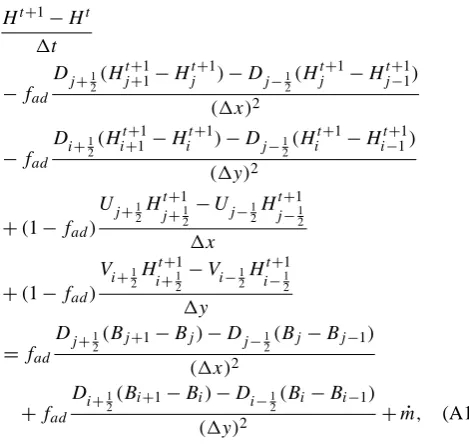
For the the A-grid a pure advective scheme to solve Eq. (31) would be numerically problematic, because of the velocity– pressure gradient coupling. Hence, we decompose the equa-tion into a weighted advective and diffusive part by apply-ing the identity(∇H+∇B)(∇S)−1=1, derived from a sim-ple gradient formulation ofS=H+B (surface elevationS

equals ice thicknessHplus ice bottomB):

∂H

∂t + fad ∇ ·

h

ViH (∇S)−1(∇H+ ∇B)

i

+(1−fad)∇ ·(ViH )= ˙m, (36)

withfad=1 for pure diffusion andfad=0 in case of pure

advection. With the definition of the non-linear (because

it depends on the solution H) diffusion vector Di :=

(Dx, Dy)= −ViH (∇S)−1we derive

∂H

∂t −fad∇ ·(Di∇H )+(1−fad)∇ ·(ViH )

=fad∇ ·(Di∇B)+ ˙m. (37)

The finite difference formulation of Eq. (37) as well as the coefficientsCnm for the sparse linear matrix for the interior

and the boundary conditions are given in the Appendix A. In general, it would be appropriate to apply the diffusive equation (with fad=1), because a Lax method has to be

used to numerically stabilise the advective part of Eq. (37) (see Appendix A). Unfortunately, this adds numerical dissi-pation (numerical diffusion) and results in a time-step depen-dence of the solution. However, if the ice body contains ice shelves and/or ice divides with flat areas, the reciprocal value of(∇S)−1becomes very large and counteracts the stabilis-ing effect of the otherwise stable diffusive implementation. Despite this problem of exchanging stability towards conver-gence (with respect to decreasing time steps) this approach has been discussed in some applications (e.g. Pattyn et al., 2006; Docquier et al., 2011).

As an alternative to overcome the restrictions involved with the numerical representation with respect to (∇S)−1

in Eq. (36), we implemented a mass conserving (time step independent) upwind scheme, based on Eq. (34). Averag-ing the horizontal velocities from their central (A-grid) loca-tion towards the grid-cell edges according toU_i,jc =1

2(Ui,j+

Ui,j+1)andV_i,jc =₂1(Vi,j+Vi+1,j)leads to

H_i,jt+1+ 1t 21x

h

U_i,jc + |U_i,jc |

H_i,jt+1+

U_i,jc − |U_i,jc |

H_i,jt+1₊₁

−U_i,jc ₋₁+ |U_i,jc ₋₁|H_i,jt+1₋₁−U_i,jc ₋₁− |U_i,jc ₋₁|H_i,jt+1i

+ 1t 21y

h

V_i,jc + |V_i,jc |H_i,jt+1+V_i,jc − |V_i,jc |H_it₊₁+1_,j

−

V_ic₋₁_,j+ |V_ic₋₁_,j|

H_i,jt+1−

V_ic₋₁_,j− |V_ic₋₁_,j|

H_it₋₁+1_,j

i

=H_i,jt + ˙m1t, (38)

and the following coefficients for the sparse matrixAnm:

Cn1= −

1t

21y(V

c

i−1,j+ |Vic−1,j|),

Cn2= −

1t

21x(U

c

i,j−1+ |Ui,jc −1|),

Cn3=1+

1t

2

(U_i,jc + |U_i,jc |)−(U_i,jc ₋₁− |U_i,jc ₋₁|)

1x

+(V

c

i,j+ |Vi,jc |)−(Vic−1,j− |Vic−1,j|)

1y

!

,

(9)

M. Thoma et al.: Description of the ice flow model RIMBAY 9 Cn4= +

1t

21x(U

c i,j− |U

c i,j|),

Cn5= +

1t

21y(V

c i,j− |V

c i,j|),

bn=Hi,jt + ˙mi,j1t. (39)

4.4 Ice sheet–ice shelf coupling and grounding line flux

The mechanically correct way of coupling a ice sheet system with an ice shelf system would be a FS approach. Accord-ing to Pattyn et al. (2013) a horizontal resolution of less than 0.5 km is necessary to capture the grounding line (GRL) mi-gration accurately. This however, is computationally costly and inefficient, especially for major parts of the ice sheet and ice shelf, which are at a large distance from the GRL where reduced physics is sufficient (see Eqs. 16 and 18, re-spectively). Either a finite element discretisation (as in the Elmer/ice model or the Ice Sheet System Model (ISSM), e.g. Zwinger et al., 2007; Larour et al., 2012) or a finite volume approach are necessary to implement FS physics in a reason-able way. Another approach to increase the grid resolution in specific regions of interest are adaptive grids (e.g. Gladstone et al., 2010; Cornford et al., 2013), although they have (to our knowledge) not been applied to HOM or FS physics, yet. For coarse resolution finite difference models (with grid sizes beyond one kilometre), Pollard and DeConto (2009) and Pollard and DeConto (2012) suggested a heuristic ap-proach, based on the semi-analytical grounding line flux so-lution, derived by Schoof (2007):

QS_x= A (ρg)

n+1₍₁₋_ρ/ρ Ocean)n 4n_C

!_m1₊₁

_τ0

xx

τf

_mn₊₁

h

m+n+3

m+1

g , (40)

with the longitudinal stress τ_xx0 just downstream of the grounding line, and the unbuttressed stress τf =

0.5ρghg(1−ρ/ρOcean). The grounding line flux QSx is

es-timated from the ice thicknesshgat the interpolated sub-grid

grounding line position. Before the ice evolution Eq. (30) is solved, the Schoof flux (estimated on a sub-grid scale) con-strains the flux across the grounding line by correcting the previous estimated velocity, located on a discrete grid node according to

u=Q

S x

H v=

QS_y

H A-grid,

u= 2Q

S x

H+Hfloat

v= 2Q

S y

H+Hfloat

C-grid. (41) With the ice thickness H at the last grounded node (the model’s grounding line) andHfloat the ice thickness at the first floating node downstream. The distinction depends on the relation between the analytical Schoof-fluxQS_i and the

modelled flux through the last gridded nodeQM_i =ViH (or

QM_i =Vi·0.5(H+Hfloat) on a C-grid): if QS_i ≥QM_i then more ice is transported into the ice shelf and the grounding line retreats or stays constant, the velocity at the grounding line is corrected according to Eq. (41). IfQS_i < QM_i then less ice is transported into the ice shelf and more ice is kept in the ice sheet, the grounding line advances and the velocity of the first floating node is corrected according to Eq. (41). A detailed description of this method is given in Docquier et al. (2011), Pollard and DeConto (2012), and Pattyn et al. (2012). To avoid unrealistic velocity steps, we additionally apply a conservative 2D-Gaussian filter to the grounding line nodes to smooth the resulting velocity field.

5 Implementation

5.1 General Information

The RIMBAYcode is mainly2written in C++ and has about 30 000 (mostly) well documented lines. For historical rea-sons the code is not completely object oriented yet, the ma-jority is organised into classes, and the number of global vari-ables (which should be avoided as much as possible in any code) is close to zero. A reasonable degree of code separa-tion into several C++ classes, allows an easy maintenance of the code. Well-defined interfaces (public methods of the C++ classes) enable an easy extension of the code for upcoming developments in ice modelling and/or further reaching appli-cations (see Sect. 7).

The GNU build system3(also known as the autotools) is a suite of programming tools designed to assist in making source-code packages portable to many Unix-like systems. It generates system- and environment-dependent Makefiles automatically and attends dependencies between different source (and header) files. Thanks to the GNU build system, RIMBAYhas been compiled and tested successfully on sev-eral different Unix-platforms without any code adjustments. To distribute, develop, and maintain RIMBAY we use the distributed revision control system monotone4, which keeps track of any changes within the code and provides a sophis-ticated automatic merging of development branches.

One of the main programming paradigms for RIMBAYis that the very same (compiled) code has to run every single (previous successfully tested) scenario without any code edit-ing and/or recompiledit-ing. To achieve this, RIMBAY is started with command-line arguments and loads the specific sce-nario from parameter files and (if requested) optionally from a netcdf file, too. The well established netcdf output format of 2_{A few parts of R}_IMBAY _{are still based on the original code}

of Pattyn (2003, 2008), which was written in C and not C++; also the implemented solver libraries (from NR and LIS), and the netcdf interface are written in C.

(10)

RIMBAYensures that the computed results can subsequently be post-processed with the desired software packages, if the supplied GMT-bash scripts (Wessel and Smith, 1998; Wessel et al., 2013) (included in the RIMBAY-monotone database) should not be sufficient.

The RIMBAY code comes with a test suite containing nearly 50 different scenarios. These small and fast-running scenarios are designed to ensure that future model develop-ments do not interfere with previous results.

5.2 Solver coupling

The coupling of SIA and SSA at the grounding line is re-alised by applying depth averaged velocities from the SIA solver as a Dirichlet boundary condition for the SSA solver. This transition can be located either at the last grounded node (the numerical GRL) or several grid nodes inside the ice sheet. In the latter case a transition zone (or grounding zone) is defined by a region where the solutions of the SIA and the SSA solvers are interpolated.

If the HOM/FS should not be applied to the whole model domain (which might be reasonable to save computational time), one or more region(s) of interest can be defined. In that case, the resource-consuming HOM/FS solver is limited to these regions only, while the faster SIA and SSA solvers are applied elsewhere and provide the Dirichlet boundary condi-tions for the HOM/FS solver (see example in Sect. 6.4).

6 Validation

The implementation of the different mathematical models (SIA, SSA, HOM, and FS) to calculate the horizontal veloc-ity field are validated separately in this subsection. Addition-ally we show that the solver for the ice sheet evolution and the solver coupling produces reasonable results. The temper-ature evolution and thermomechanical coupling is not recon-sidered here. Although the solvers have been revised, their results are identical to those published by Pattyn (2003) and Thoma et al. (2012).

6.1 SIA solver

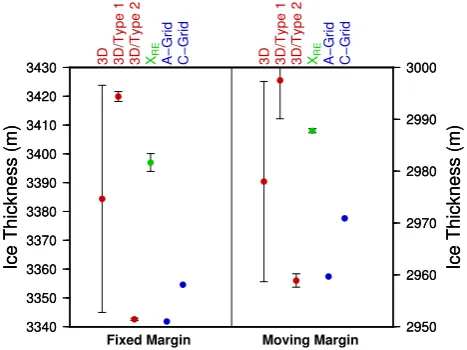
The A-grid implementation of the SIA within RIMBAY is mainly identical to those of Pattyn (2003) and has already been validated successfully against the moving-margin Eis-mint benchmark described in Huybrechts et al. (1996) within Pattyn (2003). Here, we compare the estimated ice thick-nesses, derived with the A-grid (Type-II according to Huy-brechts et al., 1996) and the C-grid RIMBAYimplementation for the fixed- and moving-margin benchmark experiments, with results published by Huybrechts et al. (1996) and Bueler et al. (2005). Figure 5 shows that the A-grid implementa-tion produces results very close to the reference, while the C-grid implementation results in a 0.38 % larger ice thick-ness. Considering the very different discretisations (compare

3D 3D/Type 1 3D/Type 2 XRE A−Grid C−Grid

Fixed Margin

3340 3350 3360 3370 3380 3390 3400 3410 3420 3430

Ice Thickness (m)

3340 3350 3360 3370 3380 3390 3400 3410 3420 3430

Ice Thickness (m)

3D 3D/Type 1 3D/Type 2 XRE A−Grid C−Grid

Moving Margin 2950

2960 2970 2980 2990 3000

Ice Thickness (m)

2950 2960 2970 2980 2990 3000

Ice Thickness (m)

Fig. 5.Comparison of modelled SIA ice thicknesses of experiments

described in Huybrechts et al. (1996) (red), theRichardson extrap-olationresult of Bueler et al. (2005) (green), and RIMBAYresults (blue). The RIMBAY A-Grid implementation corresponds essen-tially with the 3D/Type-II.

6.1 SIA–Solver

405

The A-Grid implementation of the SIA within RIMBAY is

mainly identical to those of Pattyn (2003) and has already

been validated successfully against themoving-margin

Eis-mintbenchmark described in Huybrechts et al. (1996) within

Pattyn (2003). Here, we compare the estimated ice

thick-410

nesses, derived with the A-Grid (Type-II according to

Huy-brechts et al., 1996) and the C-Grid RIMBAYimplementaion

for the fixed- and moving margin benchmark experiments,

with results published by Huybrechts et al. (1996) and Bueler et al. (2005). Fig. 5 shows that the A-Grid

implementa-415

tion produces results very close to the reference, while the C-Grid implementation results in a 0.38% larger ice thick-ness. Considering the very different discretisations (compare Eq.34 and Eq. A2) of the ice evolution equation, this is ac-ceptable.

420

6.2 SSA–Solver

The A- and the C-Grid implementations of the SSA are com-pared with a diagnostic tabular iceberg experiment of Jansen et al. (2005). In this experiment, the horizontal velocity field of a rectangular iceberg with a constant thickness of 250 m

425

and an isothermal temperature of−20◦_{C is calculated. The}

viscosity is calculated according to Eq.8 with n = 3and

a temperature dependent rate factor given by the Arrhenius relationship after Paterson and Budd (1982). Our horizontal velocities are calculated on a 1 km grid and are in close

agree-430

ment with those presented by Jansen et al. (2005) (Fig.6a). Additionally, we rotate the iceberg, to demonstrate the inde-pendence of the model results from the iceberg’s orientation

4

http://www.monotone.ca/

within the rectangular grid 6b-e. This test is essential for the modelling of evolving ice sheet fronts, which are rarely

435

aligned with the grid orientation in real geometries.

A much more complex proof-of-concept is shown in Fig.7. This artificially constructed geometry with a grid resolution of 2 km features

– a non-constant ice thickness,

440

– two discontinuous areas, which are solved

simultane-ously by the numerical solver,

– a quite complex shaped ice-water front with corners,

tongues, and an inlet atx≈200km.

– The brown areas in Fig.7 symbolises nunataks, where

445

special boundary conditions are applied: In the south

(y = 0), a no-slip boundary results in stagnation at

the ice-nunatak interface, while at the northern edge

(y = 220km) of the right iceberg a free-slip boundary

condition is applied.

450

– Additionally, a small nunatak (with an area of10km×

5km = 50km2) located within the left iceberg with

free-slip boundary conditions is added.

The modelled velocity pattern is consistent with the expecta-tions, which are

455

– higher velocities at higher ice fronts,

– zero velocities at no-slip boundaries, and

– a reduced, orthogonally orientated velocity field at

free-slip boundaries.

The difference between the A-Grid and the C-Grid (not

460

shown) are negligible. Therefore, we conclude that the SSA-solver implementations produces reasonable and robust re-sults, even for complex geometries.

6.3 SIA–SSA–solver coupling and GRL-Migration

The results of theMarine Ice Sheet Model Intercomparison

465

Project(MISMIP) (Pattyn et al., 2012) are a good benchmark

test for the capability of a coupled ice sheet/shelf model to predict grounding line migrations. In this 2D–flowline exper-iment the position of the GRL is compared with the boundary

layer theory of Schoof (2007). We applied RIMBAYwith

dif-470

ferent horizontal resolutions and a transition zone of 100 km, imposing the heuristic condition according to the method described in section 4.4. Figure 8 indicates, that the semi-analytical steady state grounding-line positions, according to the boundary layer theory of Schoof (2007), are in general

re-475

produced well with RIMBAY. However, some delayed

move-ments happen, because of numerical issues in this idealised set up.

Recently, RIMBAYparticipated in the extended 3D-variant

of the Marine Ice Sheet Model Intercomparison Project

480

(MISMIP), which investigates the grounding line response to external forcings (Pattyn et al., 2013). We performed different scenarios with a comparable coarse resolutions be-tween 2 and 20 km, because our main focus was on the appli-cability of these approximations with respect to large-scale

485

Fig. 5. Comparison of modelled SIA ice thicknesses of experiments

described in Huybrechts et al. (1996) (red), the Richardson

extrap-olation result of Bueler et al. (2005) (green), and RIMBAYresults

(blue). The RIMBAYA-grid implementation corresponds essentially with the 3D/Type-II.

Eqs. 34 and A2) of the ice evolution equation, this is accept-able.

6.2 SSA solver

The A- and the C-grid implementations of the SSA are com-pared with a diagnostic tabular iceberg experiment of Jansen et al. (2005). In this experiment, the horizontal velocity field of a rectangular iceberg with a constant thickness of 250 m and an isothermal temperature of −2◦C is calculated. The viscosity is calculated according to Eq. (8) with n=3 and a temperature dependent rate factor given by the Arrhenius relationship after Paterson and Budd (1982). Our horizontal velocities are calculated on a 1 km grid and are in close agree-ment with those presented by Jansen et al. (2005) (Fig. 6a). Additionally, we rotate the iceberg, to demonstrate the inde-pendence of the model results from the iceberg’s orientation within the rectangular grid (Fig. 6b–e). This test is essen-tial for the modelling of evolving ice sheet fronts, which are rarely aligned with the grid orientation in real geometries.

A much more complex proof-of-concept is shown in Fig. 7. This artificially constructed geometry with a grid res-olution of 2 km features

– a non-constant ice thickness;

– two discontinuous areas, which are solved simultane-ously by the numerical solver;

– a quite complex shaped ice–water front with corners, tongues, and an inlet atx≈200 km.

– The brown areas in Fig. 7 symbolise nunataks, where special boundary conditions are applied: In the south