An on‑line processing strategy for head
movement interferences removal of dynamic
brain electrical impedance tomography based
on wavelet decomposition
Ge Zhang
1,2†, Weichen Li
2†, Hang Ma
2, Xuechao Liu
2, Meng Dai
2, Canhua Xu
2, Haoting Li
2, Xiuzhen Dong
2,
Xingwang Sun
1*and Feng Fu
2*Abstract
Background: Head movement interferences are a common problem during
pro-longed dynamic brain electrical impedance tomography (EIT) clinical monitoring. Head movement interferences mainly originate from body movements of patients and nursing procedures performed by medical staff, etc. These body movements will lead to variation in boundary voltage signals, which affects image reconstruction.
Methods: This study employed a data preprocessing method based on wavelet decomposition to inhibit head movement interferences in brain EIT data. Mixed Gauss-ian models were applied to describe the distribution characteristics of brain EIT data. We identified head movement signal through the differences in distribution character-istics of corresponding wavelet decomposition coefficients between head movement artifacts and normal signals, and then managed the contaminated data with improved on-line wavelet processing methods.
Results: To validate the efficacy of the method, simulated signal experiments and human data experiments were performed. In the simulation experiment, the simulated movement artifact was significantly reduced and data quality was improved with indi-cators’ increase in PRD and correlation coefficient. Human data experiments demon-strated that this method effectively suppressed head movement in signals and reduce artifacts resulting from head movement artifacts in images.
Conclusion: In this paper, we proposed an on-line strategy to manage the head movement interferences from the brain EIT data based on the distribution characteris-tics of wavelet coefficients. Our strategy is capable of reducing the movement interfer-ence in the data and improving the reconstructed images. This work would improve the clinical practicability of brain EIT and contribute to its further promotion. Keywords: Brain electrical impedance tomography, Head movement, Wavelet decomposition, Gaussian distribution, Brick-laying algorithm
Open Access
© The Author(s) 2019. This article is distributed under the terms of the Creative Commons Attribution 4.0 International License (http://creat iveco mmons .org/licen ses/by/4.0/), which permits unrestricted use, distribution, and reproduction in any medium, provided you give appropriate credit to the original author(s) and the source, provide a link to the Creative Commons license, and indicate if changes were made. The Creative Commons Public Domain Dedication waiver (http://creat iveco mmons .org/publi cdoma in/zero/1.0/) applies to the data made available in this article, unless otherwise stated.
RESEARCH
*Correspondence: [email protected]; [email protected] †Ge Zhang and Weichen Li contributed equally to this work
Background
Dynamic brain electrical impedance tomography (EIT) is a non-invasive, low-cost, continuous monitoring functional imaging technology used in the biomedical field, which has applications for early diagnosis of cerebrovascular disease. Usually, the EIT system uses 16 electrodes placed uniformly on the head to apply safe currents and measures boundary voltage at two different instants, then reconstructs intracranial impedance changes between the two instants according to Acerta in algorithm [1,
2]. To ensure that their constructed image is accurate, the boundary voltage varia-tion between the reference frame and current frame should originate from changes in intracranial impedance. Thus, good and stable connection between electrodes and the scalp is a crucial factor for image monitoring of brain EIT. However, dynamic brain EIT monitoring is a long-term process. The change of connection status is a com-mon occurrence during our previous clinical studies because of factors like: patient’s body movements (head rotation, body turning) and nursing procedures performed by medical staff. These body movements lead to head movements and change the elec-trode–skin contact status, which introduce movement interferences in data collection and image reconstruction [3, 4]. Therefore, there is an urgent need for appropriate methods to process the movement interferences if we want to further promote the dynamic brain EIT research.
Impedance mapping, EEG, near-infrared spectroscopy, and other similar techniques also encounter body movement interference problems during clinical practice. Sev-eral methods for movement interference removal in such electrical signals have been reported. These methods can be mainly classified into two types.
The first type is based on adaptive filters. In this occasion, additional input signals are required for movement artifacts removal. Researchers acquired the expected signal or interference by set extra measurement channel in the hardware [14–16].
The second type mainly includes Wiener filter methods, signal-related improvement methods and Kalman filter method, which does not need additional input. The wie-ner filter requires the acquisition of a priori information of expected signals, like sig-nal’s power spectrum [17]. The signal improvement method was proposed by Cui et al. [18]. The disadvantage is that the expected signal and interference should be maximally negatively correlated if possible. The Kalman filter method requires a priori information models in which noise distribution is obtained [19]. Besides, there are also the principle component analysis (PCA) method [20], independent component analysis (ICA) method [21], spline interpolation method [22], etc., which all have particular scope of applica-tion and limitaapplica-tions in real-time processing. Therefore, these methods are not ready for removal of movement interferences in dynamic brain EIT.
Wavelet decomposition is a signal processing method that analyzes the time–fre-quency characteristics of signals to detect and process body movement interference components. As there are differences in amplitude and duration between head move-ment interferences and normal photoelectric signals, these differences could be distin-guished and managed in wavelet domain. Wavelet method shows good performance when processing weak signals, and provides us with referential application in dynamic brain EIT. However, the literature reporting use of this method does not mention spe-cific real-time processing [14, 23–25].
Based on the points above, our study took advantage of the differences in the distribu-tion characteristics of brain EIT signals and movement interference signals in wavelet domain to extract and process the movement interference signals by employing event probabilities. Meanwhile, brick-laying algorithm strategies were used to achieve on-line operation of this processing strategy.
In this scenario, the patients suffer from brain injury and have to stay lying on the sickbed in supine position. They will keep the supine position after any initiative or pas-sive head movement for comfort or medical consideration. The status of affected elec-trodes will be switched between being pressed and released. This kind of movement interferences may not result in data acquisition failure, but contaminate the brain EIT signal with spike-like artifacts. The spike-type movement interferences are the objects to manage in our study.
Methods
EIT data acquisition procedures
entry and exit electrodes, respectively, while electrodes 0–1, 1–2, 2–3…15–0 were used as measurement electrode pairs to obtain 16 sets of voltage differences. The above steps were repeated by injecting by injecting the current through electrode pair 1–9, 2–10,…, 15–7 sequentially and all adjacent measurements constituted one frame of data (256 sets) [26]. While the measurements adjacent to the excitation electrode contain more contact impedance than internal impedance and need to be discarded during recon-struction, there are 16×(16−4)=192 valid measurements in each frame. Therefore,
there are 192 data channels that require observation and processing [27].
Influences of head movement interferences on boundary voltage
The EIT image reconstruction process can be briefly summarized as:
where x represents input data, which is a frame of boundary voltage data, y represents the conductivity distribution of the target field, and B is the construction matrix which is
determined by the finite element model (FEM) of the target field, and is closely related to the number of model elements, number of boundary measurement values, background conductivity, electrode model, etc.
With respect to dynamic EIT, the reconstruction process can be briefly described as:
where xf represents the boundary voltage measurement data of the current frame and xb
represents the boundary voltage measurement data of the reference frame. Under nor-mal circumstances, the assumption is that differences in xf and xb only originate from
changes in intracranial impedance.
When the electrode contacts the scalp, electrode–scalp contact impedance unbalance occurs [28, 29]. During brain EIT detection, contact impedance affects measurements in two ways: first, when electrodes are used as the measurement tool, the presence of electrode–scalp contact impedance is equivalent to the addition of a conductive layer outside the normal field. It will affect current distribution beneath the electrode. In addi-tion, if contact impedance is sufficiently large, it will affect the common-mode rejection
(1)
y=Bx
(2)
y=B(xf−xb)
ratio at the measurement end [30, 31]. Second, the contact impedance may decrease the injected current when the electrodes act as excitation pair. Therefore, the head move-ment leads to artifacts into EIT signal [32]. These contact impedance variations only occur in the current frame and result in image artifacts. Since the movement duration is shorter than the voltage changes caused by intracranial pathophysiological changes, it is characterized by rapid changes in EIT signal. And due to the high resistivity of the skull compared to the degree of intracranial impedance changes, the ratio of corresponding boundary voltage changes is far smaller than the changes in intracranial impedance. Thus, it can be concluded that the head movement disrupts the continuity of EIT signals, which is equivalent to high-frequency outlier in stable signals. This makes it possible to use wavelet analysis methods to discriminate normal signals and from head movement interferences.
Processing strategy for head movement interferences based on wavelet decomposition
In previous analyses, the movement interference signals are considered as sudden changes with larger amplitude values in stationary signal. In contrast, slowly changing boundary voltage signals caused by internal impedance changes are regarded as low-frequency signals. In the wavelet domain, the low-low-frequency components correspond to wavelet coefficients in smaller values and the high-frequency components correspond to wavelet coefficients in larger values. So we can discriminate normal signals from movement interferences in temporal manner through wavelet decomposition [33, 34]. Especially, in the scenarios where normal components and interferences are aliasing in frequency domain, the wavelet strategy is able to exert its time–frequency analysis fea-tures and achieve better results.
Original signal s(t) can be expressed as:
where s0(t) represents EIT signals without head movement interferences and ε(t) rep-resents head movement interference signal. The Mallet method was used to carry out wavelet decomposition, and raw signals can be expressed as [35, 36]:
where φjk(t)=2j/2φ (2jt−k) represents the function of the reconstruction scale,
ψjk(t)=2j/2ψ (2jt−k) represents the reconstructed wavelet function, j and k represent the number of layers and scale translation coefficient in wavelet decomposition, respec-tively, v represents the scale decomposition coefficient, and wj represents the wavelet
decomposition coefficient at the j th level. In addition,
where j=j0,. . .,J−1,k=0,. . ., 2J−1,g(l−2k) is a high-pass filter, and h(l−2k) is a
low-pass filter. The corresponding wavelet coefficient at the first level is:
(3) s(t)=s0(t)+ε(t)
(4)
s(t)=
k
vj0kφj0k(t)+
j=j0
k
wjkψjk(t)
(5) wjk =
l
g(l−2k)vj+1(l)
(6) vjk =
l
Combining the above methods, the corresponding decomposition coefficient can be written as:
The coefficients for various layers in top-down decomposition coefficient can be expressed as:
The movement interference management based on wavelet method is achieved by dealing with the detailed wavelet coefficients. The normal brain EIT signals are continu-ous and relatively smooth and slow-changing [37–39]. Compared with the head move-ment interferences, the corresponding wavelet decomposition coefficients are small fluctuations concentrated around zero. This characteristic can be used to carry out dis-crimination and processing head movement interference signals. We adopted Molavi’s wavelet processing strategy to manage the movement interferences [23].
Once a segment of signal is decomposed by wavelet function, the wavelet coefficients can be represented by a Gaussian mixture model containing two zero-mean Gaussian distributions [40]. One Gaussian distribution describes large wavelet decomposition coefficients, while the other Gaussian distribution describes the remaining small coef-ficients. Among these coefficients, larger coefficients correspond to dramatic signal changes and the corresponding Gaussian distribution is relatively dispersed. Then the large coefficients can be set to zero to inhibit dramatic changes in signals. Giving the probability density function of Gaussian distribution with smaller variation, we can cal-culate the geometric probability of wavelet coefficients. We define rejection probability to present this geometric probability. Considering the wavelet coefficient wjk,s0 of signals
can be represented by wjk,s0 ∼N(0,σ2), the definition of rejection probability is:
where φ (k)= 1 ˆ
σ√2π
k −∞e
−k2
2σˆ2dk is the Gaussian probability density function. If the wavelet decomposition coefficient does not originate from the Gaussian distribution with smaller variation, the calculated rejection probability should be higher than the ones that comply with this distribution. We can set threshold α to pick out and manage
the wavelet coefficients of head movement interferences. The management strategy is: (7)
w1k =
l
g(l−2k)s(l)
(8)
v1k =
l
h(l−2k)s(l)
(9) w1k =w1k,s0+w1k,ε
(10)
v1k =v1k,s0 +v1k,ε
(11)
wjk =wjk,s0+wjk,ε
(12) vjk=vjk,s0+vjk,ε
(13) pjk=
φ wjk
ˆ σ −0.5 ∗2 (14) wjk =
0 wjk
wjk containing head movement will be larger and less possibly belong to the assumed N
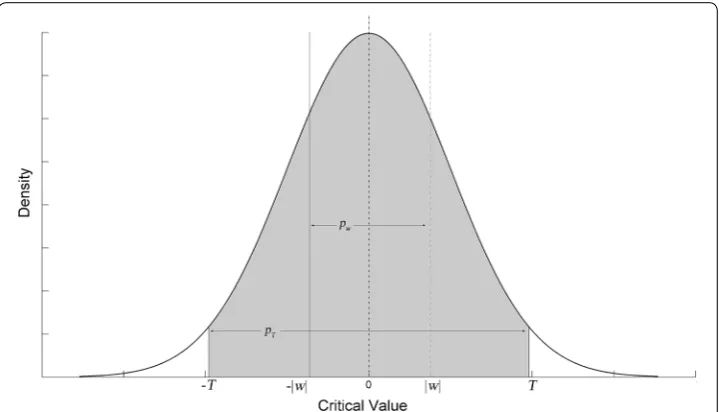
distribution. It will be set to zero to suppress interference in reconstruction signals. Fig-ure 2 illustrates this concept. Once the movement interferences in the brain EIT signal are suppressed, the resulted artifacts in the EIT images will be removed consequentially.
On‑line calculation for wavelet processing strategy
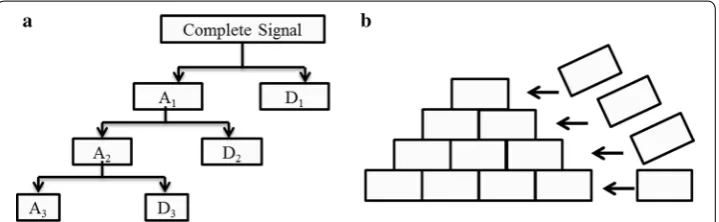
The Mallet method is usually used for discrete wavelet decomposition. It is based on multi-resolution analysis, wherein high- and low-pass filters are used recursively to achieve the projection of any signal on scale space using a scale function as an orthogo-nal basis, and on a wavelet space using wavelet function as an orthogoorthogo-nal basis. Nor-mally, it is essential to acquire all data in advance to carry out wavelet decomposition. That is so-called pyramidal algorithm. All data are first read to construct the first layer of the pyramid and the values of the scale coefficient and wavelet coefficient of the first layer are calculated before calculating the second layer. The algorithm progresses layer by layer until reaching the required level. Therefore, data reconstruction can only be carried out after all decomposition is completed and wavelet decomposition and recon-struction are not carried out in real-time.
In the theoretical analysis of multi-resolution, the support length of the scale function is not stipulated as finite length or infinite length. But in practical calculation, the sup-port length of wavelet function is limited. Therefore, the decomposition filters are with finite length and only able to convolve limited data. So in the wavelet decomposition, there is no need to complete the calculation of the entire bottom layer before calculating the upper layer. The Mallet method can be modified [41]: we can perform once convo-lution in the higher decomposition level after twice convoluting in the lower level. The
Fig. 2 Illustration of the wavelet decomposition coefficients’ rejection probability and its comparison with threshold probability. For coefficient w , its corresponding rejection probability is pw , which is the integration
from −|w| to |w| with assumed Gaussian probability density function. T is the threshold of w and pT is
corresponding threshold of pw . If w is artifact-free, the coefficients are spread around zero. Then the pw will be
less than pT . If w is contaminated with movement artifacts, the coefficients will be discretely distributed and
whole calculation is performed transversely and upward. The higher layer convolution can be calculated as long as the lower layer offers data long enough to perform one cal-culation. So we do not need to acquire all signal data to perform wavelet decomposition. Unlike the pyramidal algorithm, this kind of calculation is more akin to brick-laying. Fig-ure 3 shows specific operations compared with conventional operations.
Data processing parameter selection
The movement interference management based on wavelet method requires the confir-mation of multiple parameters, including wavelet function, number of decomposition layers, screening threshold, and variance of the priori Gaussian distribution. The vari-ance of the normal distribution is determined as the median absolute deviation in the decomposition coefficient sequence. The median absolute deviation has good robustness and is not sensitive to small numbers of outliers in the extraction sequence. In dynamic brain EIT measurements, head movement interferences present as individual outliers with high amplitude. Therefore, when median absolute deviation is used to estimate the variance, the result will not be sensitive to a few head movement interferences. The cal-culation for the distribution variance of the wavelet coefficient at each layer is [24, 42]:
We need to determine the wavelet function based on the morphological and empirical choice. Considering that the majority of head movement interferences appear as spikes and limited filter length is required for real-time operations, db4 wavelet was used for signals’ decomposition and reconstruction. According to reports in which wavelet decomposition was used for signal processing, when decomposition reaches the fourth layer, processing results from further decomposition does not show any significant dif-ferences when compared with processing results at the fourth layer of decomposition. Differential probabilities with statistically significant differences were used as a reference for the selection of filtering threshold. When the corresponding adaptive probability of the current w is greater than 90% (i.e., the probability that w falls into the a priori normal
distribution is greater than 90%), the source of w does not include measurement signals
that contain head movement interferences (i.e. α=0.9).
(15) ˜
σj= Median
Wj
0.6745
Experiment validation design
To validate the feasibility of the proposed approach, we performed experiments with simulated data, phantom data and clinical measurement. The simulations and data processing were performed in Matlab version 2012b. All imaging reconstructions were implemented in self-developed software developed by C++.
Real EIT data were collected using an EIT system (FMMU-EIT5) [43]. This system uses a working frequency at 1–190 kHz, excitation current ranges from 500 to 1250 μA with measuring accuracy of 0.01%. The common-mode rejection ratio is over 80 dB. The image reconstruction algorithm was the damped least-squares algorithm developed by our research group [37]. We have used this system for previous clinical studies on brain EIT [44, 45]. In this study, we employed 500 μA and 50 kHz altering current to collect human data with the speed of 1 frame/s. All calculation were implemented on a Pentium G630 computer.
Simulation experiments
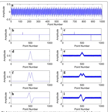
The ideal brain EIT signals can be regarded as direct current signals. Therefore, while generating signals, we need the simulation containing similar typical changes of the EIT signal. We used the following equation to generate a segment of composite frequency sinusoidal signal with white Gaussian noise:
where n=4,ω=2πf,µ represents the oscillation amplitude of the sine wave, σ (t)
rep-resents the Gaussian white noise, γ represents the amplitude of the Gaussian white noise,
and the amplitude range for xsimulate(t) is (−1, 1) . The frequencies and amplitudes of the
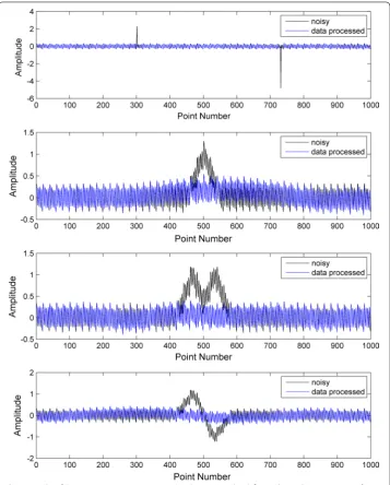
four types of sine waves used were (1 Hz, 0.6), (0.1 Hz, 0.9), (0.25 Hz, 0.9), (0.04 Hz, 1) and a total of 1000 data points were set, which were used to generate signals as shown in Fig. 4.
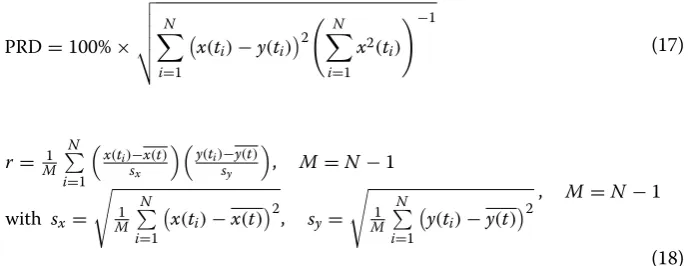
Spike signals simulating head movement interferences were added to the generated simulation signals to evaluate the consistency of post-processed and raw simulation signals. Evaluation was carried out using the three indicators of percent root difference (PRD), Pearson product–moment correlation coefficient (r), and coefficient of determi-nation (R-square) [22].
(16) xsimulate(t)=
1 3
n
i=1
µisin(ωit)+0.05σ (t)
(17)
PRD=100%×
N
i=1
x(ti)−y(ti)
2 N
i=1 x2(t
i)
−1
(18) r= M1
N
i=1
x(ti)−x(t)
sx
y(ti)−y(t)
sy
, M=N−1
with sx =
1 M
N
i=1
x(ti)−x(t)
2 , sy=
1 M
N
i=1
y(ti)−y(t)
2
Here we consider x(t) as original signal without movement interference. PRD evalu-ates the consistency between x(t) and y(t) while r and R-square evaluate the similarity
between x(t) and y(t).
Physical phantom experiments
The physical phantom experiments were carried out on a resistor phantom representing a circular homogeneous medium and comprised of 120 resistors (1 kΩ) with 0.1% preci-sion [46]. The phantom was connected to the data collection system through the SCIS-36 port [10]. Localized conductivity perturbation could be generated by operating the 16 push-type switches on the phantom. The finite element model for image reconstruc-tion was a homogeneous circular mesh with 288 triangle elements. First, we acquired frames of EIT data without imaging target as the reference frames, and continued the (19) R-square=
N
i=1
y(ti)−x(t)2
N
i=1
x(ti)−x(t)
2
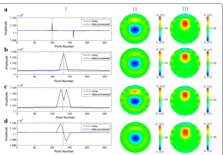
data collection after pushing one switch to produce one conductivity perturbation as current frames. We simulated four different spike interference scenarios by adding dif-ferent spikes on the current frame part of phantom data.
Human measured data experiments
The clinical data were acquired in the neurosurgery ICU of Xijing Hospital, Fourth Mili-tary Medical University, Xi’an, China. This study was approved by the human research ethics committee of the Fourth Military Medical University and informed written con-sent was obtained from the patient’s nearest relatives. In this scenario, two male patients were included. One patient suffered from head impact and had the risk of secondary injury. The other one was with cerebral edema and received mannitol dehydration treat-ment. There was no wound in the superficial scalp and all electrodes could be deployed. Both patients were conscious and lay on the sickbed. In the data collection process, no intervention was involved except for the patients’ movements themselves and nursing procedures performed by medical staff. Before data collection started, 16 rigorously dis-infected cup-shaped electrodes were attached with conductive paste (Ten 20 conduc-tive paste, Weaver and Company, Aurora, USA). Then, the electrodes were placed in an annular manner on the patient’s head. The finite element model for reconstruction was the same in phantom experiments.
Results
Validation with simulated data
The results of head movement processing method in simulation experiments are shown in Fig. 5 and Table 1. Db6 wavelet was used and the number of decomposition layers was 10 for all mixed signals. As shown in Fig. 5, we can see that the four kinds of sim-ulated spike interferences were effectively restrained in the presence after processing. Table 1 shows the quantitative indicators of post-processed signals. All indicators show improvement in data quality. PRD was increased by at least 48% and r advanced 43% in average. In type 1 and type 2 simulation, the R-square had sharp promotion, which indi-cates the goodness of the processed signal.
Validation with resistor phantom data
Figure 6 shows the mean values of continuous phantom data and the EIT image contain-ing conductivity perturbation target. The length of the data was almost 350 frames. Db6 wavelet with 6 decomposition layers was employed to implement the processing.
Validation with human measurement data
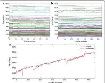
Figure 8 shows the processing results of human measurement data. One segment data of clinically measured data containing 650 frames long was selected, which included several observed head movement interferences. Db4 wavelet with 4 decomposition layers was used for data processing. Figure 8a shows the waveforms of 192 channel data in time series before processing while Fig. 8b shows the data waveforms after processing. By comparing the signal waveforms in Figs. 8a and 9b, it could be seen that the head movement interferences were reduced considerably in all channels. To demonstrate the results more specifically, we made a comparison of the mean val-ues before and after processing. Figure 8c illustrates the comparison results of mean
Table 1 PRD, r and R-square values for comparison between the simulation signals with simulated interference (type 1, type 2, type 3 and type 4) and with reduced simulated interferences (type 1-processed, type 2-processed, type 3-processed, type 4-processed)
The ∆ values correspond to percentage changes comparing the data with and without wavelet processing
PRD r R‑square ∆PRD ∆r ∆R‑square
Type 1 0.9096 0.7360 0.1726 73.28%↓ 31.81%↑ 445.18%↑ Type 1-processed 0.2430 0.9701 0.9409
Type 2 0.9753 0.7157 0.0488 48.15%↓ 24.08%↑ 1426.08%↑ Type 2-processed 0.5057 0.8880 0.7442
Type 3 1.3657 0.5904 0.8650 80.16%↓ 63.23%↑ 7.12%↑ Type 3-processed 0.2709 0.9637 0.9266
Type 4 1.3240 0.6043 0.7531 73.28%↓ 53.44%↑ 12.12%↑ Type 4-processed 0.3945 0.9273 0.8444
Fig. 6 Mean values (left side) and the normal EIT image with imaging target (right side) of the resistor phantom data
values and the single channel spikes reflecting in mean values were restrained. There-fore, our method is able to manage the spike type of movement at signal level.
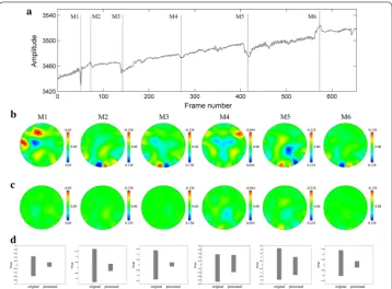
Considering EIT, an imaging monitoring technique, we testified the feasibility of proposed processing method by reconstructing the EIT images with processed data. Figure 9 shows the imaging results before and after data processing. In Row A, labels M1–M6, respectively, indicate the time locations that movement interference hap-pens. Considering the processing expectation was to inhibit head movement inter-ferences, which only exist in current frames, we selected one frame of data before movement occurrence as reference frame. Following this principle, EIT images in Row B are the reconstructed results contaminated by movement artifact. Columns M1–M6 represent that the images in this column correspond to different movements marked in Row A. The EIT images in Row C are corresponding outcome after pro-posed management. Row B shows significant artifacts introduced by head movement interferences in the reconstructed images. After signal processing by the proposed method, the artifacts are greatly reduced in corresponding EIT images of Row C. Row D indicates the variation range of reconstructed values. Because the movement usu-ally leads to outliers in the signal, the reconstruction value will be also amplified if movement interference happens. Therefore, through the downscaling of reconstruc-tion value variareconstruc-tion in row D, the artifacts in reconstructed images were suppressed effectively. All results above prove that the proposed method is able to restrain head movement interferences at signal level and image level.
Evaluation of time and storage cost
Figure 10 shows the time cost for real-time calculations in wavelet data processing. As data acquisition and data processing were carried out simultaneously, total time was significantly decreased. While the data acquisition interval is 1 s and time required for wavelet processing is far lower than 1 s, online processing is feasible.
According to the algorithms used for pyramidal method and brick-laying method, we set that wavelet data processing requirements for signals with a length of A, one layer of decomposition, wavelet filter length of N has a total number of data stored of:
(20)
Offline:A+ i=l
i=1
A
2floor(i/2)
Fig. 9 Comparison of reconstructed images with the original data and processed data. Row A is the mark of head movement occurrence, M1–M6 is the sequence number of head movement. Row B is the images reconstructed with original data. Row C is the images reconstructed with processed data. Row D is the comparison of reconstruction value range before and after data processing
Calculating the storage cost of the human measurement data in Fig. 9, the offline pro-cessing requires 1.78×10³ storage units while on-line processing only requires 130 stor-age units. Therefore, storstor-age space requirement is greatly reduced in on-line calculation.
Discussion
This paper analyzed the problem of head movement during dynamic brain EIT monitor-ing in clinical environments, and we managed the head movement interference based on the distribution characteristics of wavelet decomposition coefficients. In simulation experiments, the spikes which simulate head movement interferences were suppressed effectively after being processed by the proposed approach. The correlation between processed signal and raw signal was significantly increased, which could be concluded through the quantitative indicators such as PRD, correlation coefficient and R-square. After that, we simulated conductivity perturbation on the resistor phantom and col-lected the phantom data with spike interferences. The proposed method could remove the artifacts and restored the imaging target at the same time. To testify whether the proposed method was able to improve the clinical practicability, we collected human data in the ICU for validation. After processing, the continuity brain EIT signal was restored and movement artifacts were removed from the reconstructed images. Besides, we employed brick-laying calculation to adapt to dynamic brain EIT monitoring.
In simulation experiments, we used different types of spikes to simulate head move-ment interferences in the brain EIT signal. This choice is based on scenario analysis and actual data observation. By comparing the real movement signal, it can be seen that the spikes could well conform to the character of head movement interferences. In phantom data experiments, we demonstrated the efficacy of the proposed approach while there was simulated perturbation included in the measurement. The target information was well restored and the artifacts were suppressed effectively. In human data experiments, we could not get pure signal without movements at the same time based on existing equipment. In this way, quantitative indicators could not be calculated to measure the processing effect of real human data. Unlike the simulated signal, there were more com-ponents except for noises and spikes in the real human data, like the step-type interfer-ence, which made the processed curve less match compared with the simulations. But the further image results demonstrate the feasibility of the proposed approach. Here we only used artifact-free images to demonstrate the processing effect. There should be no voltage variation caused by intracranial pathophysiological change between the temporary reference frame and the current frame, which were a few seconds apart. The imaged targets were introduced by spike-type interference were well removed after data processing.
In previous studies, it was found that brain EIT signals showed continuity with slow changes in time series. On one hand, this is due to data acquisition speed being 1 frame/s. On the other hand, since the resistivity of the skull is high, the boundary volt-age changes caused by intracranial impedance changes are relatively small in amplitude.
(21) Online: 1+
i=l
i=1
1 2i−1
(l+1)N+2l
N
2
+
2−2l+1
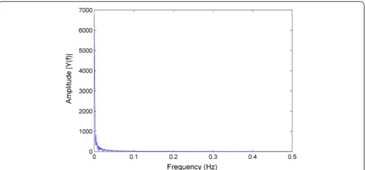
In addition, considering that intracranial pathophysiological changes that cause imped-ance changes also require some time, brain EIT signals nearly become direct current (DC) signals during a segment of frequency domain analysis. The head movement inter-ferences appear as relatively drastic changes in amplitude in an instant. Meanwhile, it takes 10 min or more time for intracranial impedance variation to result in such change in boundary voltage. Intuitively, it can be seen that normal signals and head movement interference signals show differences in frequency. However, compared with the base-line of measurement, these changes are still small in amplitude. As shown in Fig. 11, the frequency band including all head movement interferences in the entire EIT sig-nal was very narrow, and the energy of the sigsig-nal was almost concentrated at the DC segment. Thus, it is not convenient to obtain prior information of movement interfer-ences through the use of conventional digital filter methods for processing. Therefore, the frequency domains of head movement interference signals and normal signals can be considered being mixed, and only show significant distinction in the time domain. This makes characteristic time–frequency analysis methods more suitable to process the interferences. Besides, the traditional signal processing method, such as low-pass filter, separates interferences from normal signal of brain impedance variation in frequency domain. If the smoothing effect of low-pass filter is good, it will inevitably cause the sig-nal to be blurred, which means suppression of normal biological sigsig-nal. In this case, the effect of processing is at the expense of losing useful signal components. But, in signal processing by wavelet decomposition, we decompose the various frequency components in the signal into bands that do not overlap each other and only managed the parts con-taminated by movement interferences. So the normal signal of brain impedance varia-tion is left with minimum suppression.
The processing method selected in this study was based on the priori distribution information of the wavelet decomposition coefficient. If wavelet coefficient is “sparse”, i.e., the wavelet coefficient is composed of large number of small coefficients and a few large coefficients, then the Gaussian mixed distribution with two-component zero mean can effectively fit the actual wavelet coefficient distribution [47]. The differences in
these two Gaussian distributions lie in the variance. The distribution with a large vari-ance will have a low a priori probability, which represents few large coefficients; while the distribution with a small variance will have a high priori probability, representing a large number of small coefficients. The overall brain EIT detection signals are relatively smooth and slow-changing, and their wavelet decomposition coefficients can satisfy the “sparse” requirement. In addition, the characteristics of these signals are similar to previ-ously studied body movement interference signals. Therefore, the use of wavelet decom-position in this domain is reasonable [24].
During dynamic brain EIT continuous monitoring, head movement interferences will change electrode–scalp contact impedance, which will appear as changes in boundary voltage and ultimately affect image reconstruction. In previous reports, researchers have focused on the effects of contact impedance on the reconstructed images. However, such contact impedance changes often originate from conductivity changes due to elec-trochemical changes at the electrode-conductive paste–scalp contact layer. In the recon-struction process, we demonstrated that conductivity changes at the electrode contact layer are actually equivalent to impedance changes at one area in the reconstruction field. However, reconstruction algorithms themselves cannot differentiate whether volt-age changes originate from the contact layer or inside the field. Limited by the FEM use during reconstruction, these surface contact changes are regarded as impedance changes inside the field and appear as reconstruction artifacts in reconstructed images [48, 49]. Current researches mainly modify imaging algorithms with complete electrode models to isolate contact impedance changes and their effects on specific elements in the finite element model [48, 50, 51]. However, this kind of processing strategy does not consider the influences of contact impedance changes on excitation current, and can only be used to process contact impedance problems in which the magnitude of such change is smaller than head movement interferences. Previously, other studies on processing of more severe body movement interferences were targeted at extreme situations in which there is saturation or distortion of excitation current, or inability to normally enter the field. Therefore, data-abandoned processing strategies were used for affected measure-ment values. In the clinical environmeasure-ment, the movemeasure-ment interferences in the middle of the two scenarios are more common. The measurement data can still reflect the actual boundary voltage to some extent, but contains head movement inference component.
no need to care for such noise. The conversion of probability to specific threshold num-ber increased the calculation, especially such operation results were uncertain. Com-pared with other methods, that method does not need the input of any reference signal and reduces the requirement for priori information to the minimum. Compared with traditional wavelet processing methods that used fixed thresholds, the use of an adaptive probability threshold can achieve specific elastic changes in coefficient threshold and has stronger adaptability.
Our processing strategy is mainly aiming at spike-type interferences in clinical prac-tice. Patients’ movements or medical staffs’ operations will change the contact status of the electrodes. But the electrode’s contact will restore to its initial status with the elas-tic shrinkage of bandages used for fixing. In this way, head movement interferences will present as uneven spikes in the signal. The characteristic of the head movement inter-ference is no baseline alteration. The movements are discrete points in the time series. The wavelet method isolates the frequency-domain aliased interferences through its time–frequency analysis function. If the baseline is affected by movement disruption of electrode status, the processing results will be declined. That is because the data after discontinuous points show little difference compared with the normal signal in wavelet domain while it still contains baseline alteration. Therefore, the processing results with human data are a little inferior in waveform compared with the simulations. There is a special brain EIT application case, epileptic seizures imaging, where the spike-type sig-nal is monitoring target [52, 53]. The seizures are occur in tens of seconds and more like movement artifacts, which makes the seizures difficult to be separated from the real movement artifacts. Although epileptic seizures can be detected by brain EIT theoreti-cally, it is not ready for actual clinical application because of this limitation [54]. Our main object is also not epileptic seizures monitoring, so the situation that secondary sei-zures mixed with movement artifact is not included and considered in our study.
pathological process will be happening beforehand. Meanwhile, we hope to make the EIT monitoring more practical in clinical monitoring by removing the artifacts with online management. Therefore, we prefer to employ the online processing method to extend its potential application and keep as much data as possible.
While using the wavelet method to deal with head movement interference, we need to determine the variance of the Gaussian distribution and the rejection probability. To acquire the variance of the Gaussian distribution, it is necessary to acquire all wavelet decomposition coefficients of the measurement. However, this is not possible during dynamic brain EIT monitoring. Therefore, the priori variances used during on-line pro-cessing are empirical values. Although validation experiments using clinical measure-ment data have obtained satisfactory results for empirical variances, the versatility of this method requires further validation. In addition, the rejection probability threshold determines the intensity of head movement interferences that require processing. Cur-rently, to simplify the calculation, all 192 channels in EIT signals use the same threshold. However, the intensity of head movement interferences in all channels may not be iden-tical. Therefore, more optimization of choosing parameters will be done in further study. To manage the movement interference, there are some ad hoc algorithms, for instance, the compensation strategy based on spline interpolation proposed by Scholkmann [22]. Movements were detected by moving standard deviation and corrected by empirical correction value. Although the processing idea is relatively simpler, the reliability of the chosen correction value is a problem. The strategy of determining correction value lim-its lim-its application in real-time processing. As for the PCA method, it applies the simi-lar idea to separate different level of signal components based on Gaussian distribution like the wavelet decomposition does [55]. The main concern of the component lies on two aspects: first, the principle component reserved to reconstruct the signal. We need to distinguish the principle component which can represent the normal signal through eigenvalue or other mark value. While the data keep flowing, the component choice may need to be altered. Second, the real-time capability of the processing procedure. Usu-ally, the PCA is employed when all data are known. So if we want to apply the PCA to restrain the head movement in brain EIT signal, more modification on on-line calcula-tion of PCA indicators and the correccalcula-tion of the eigenvector estimacalcula-tion from theoretical level, which may make the strategy unable to act its advantage in simpler and quicker processing.
movement interference in the brain EIT measurement and quantitatively estimate the processing effect from image point.
The wavelet processing method is suitable for all time-difference EIT application theoretically. In this study, we implemented data collection with working frequency at 50 kHz and acquiring 1 frame of data per second. There is some time-difference EIT data measured at different working frequencies. And the time-difference data set is com-posed of averaged frames data to improve the accuracy of measurement. Therefore, we hope to try the proposed method on time-difference EIT data under other collection conditions and test its broadness in future work.
Conclusion
In clinical long-term dynamic brain EIT, head movement interference is a common occurrence and will lead to image artifacts. This paper offers an on-line strategy to pro-cess the contaminated measurement through wavelet decomposition. We used mixed Gaussian distribution to describe the wavelet coefficients and detected coefficients cor-responded to movement signal by distributed probability to process. Besides, modifica-tion was carried out to realize on-line processing for dynamic brain EIT monitoring. While the feasibility of this method is proved by experiments with reduced movement component, it provides an idea for data processing of brain EIT and lays a foundation for further research in data processing of brain EIT.
Abbreviations
EIT: electrical impedance tomography; FEM: finite element model; PCA: principle component analysis; ICA: independent component analysis; PRD: percent root difference; DC: direct current.
Authors’ contributions
Conceived and designed the experiments: GZWL HMXS. Performed the experiments: GZ WL. Analyzed the data: GZ HMXS. Contributed reagents/materials/analysis tools: HM XL HL CX XD FF. Wrote the paper: GZXS. All authors read and approved the final manuscript.
Competing interests
The authors declare that they have no competing interests.
Availability of data and materials
The data sets and source code of the present study are available from the corresponding author on reasonable request.
Ethics approval and consent to participate
This study was approved by the Fourth Military Medical University Ethics Committee of Human Research and informed written consent was obtained from those patients’ nearest relatives.
Funding
National Nature Science Foundation of China (Grant Number: NSFC51837011), this work is supported by National Nature Science Foundation of China (Grant Number: 51477176), National Key Technology Support Program of China (Grant Number: 2011BAI08B13) and Youth Medicine Cultivation 2016 (16QNP107).
Publisher’s Note
Springer Nature remains neutral with regard to jurisdictional claims in published maps and institutional affiliations.
Received: 27 February 2018 Accepted: 4 April 2019
References
1. Bayford R, Tizzard A. Bioimpedance imaging: an overview of potential clinical applications. Analyst. 2012;137:4635–43.
3. Hartinger AE, Guardo R, Adler A, Gagnon H. Real-time management of faulty electrodes in electrical impedance tomography. IEEE Trans Biomed Eng. 2009;56:369–77.
4. Adler A. Accounting for erroneous electrode data in electrical impedance tomography. Physiol Meas. 2004;25:227–38.
5. Vongerichten AN, dos Santos GS, Aristovich K, Avery J, McEvoy A, Walker M, et al. Characterisation and imag-ing of cortical impedance changes durimag-ing interictal and ictal activity in the anaesthetised rat. Neuroimage. 2016;124:813–23.
6. Aristovich KY, Packham BC, Koo H, Santos GS, McEvoy A, Holder DS. Imaging fast electrical activity in the brain with electrical impedance tomography. Neuroimage. 2016;124:204–13.
7. Lozano A, Rosell J, Pallas-Areny R. Errors in prolonged electrical impedance measurements due to electrode reposi-tioning and postural changes. Physiol Meas. 1995;16:121–30.
8. Adler A, Guardo R. Electrical impedance tomography: regularized imaging and contrast detection. IEEE Trans Med Imaging. 1996;15:170–9.
9. Asfaw Y, Adler A. Automatic detection of detached and erroneous electrodes in electrical impedance tomography. Physiol Meas. 2005;26:S175–83.
10. Zhang G, Dai M, Yang L, Li WC, Li HT, Xu CH, et al. Fast detection and data compensation for electrodes disconnec-tion in long-term monitoring of dynamic brain electrical impedance tomography. Biomed Eng Online. 2017;16:7. 11. Frerichs I, Amato MBP, van Kaam AH, Tingay DG, Zhao ZQ, Grychtol B, et al. Chest electrical impedance tomography
examination, data analysis, terminology, clinical use and recommendations: consensus statement of the TRansla-tional EIT developmeNt stuDy group. Thorax. 2017;72:83–93.
12. Walsh BK, Smallwood CD. Electrical impedance tomography during mechanical ventilation. Respir Care. 2016;61:1417–24.
13. Goren N, Avery J, Dowrick T, Mackle E, Witkowska-Wrobel A, Werring D, et al. Multi-frequency electrical impedance tomography and neuroimaging data in stroke patients. Sci Data. 2018;5:180112.
14. Robertson FC, Douglas TS, Meintjes EM. Motion artifact removal for functional near infrared spectroscopy: a com-parison of methods. IEEE Trans Biomed Eng. 2010;57:1377–87.
15. Zhang Q, Brown EN, Strangman GE. Adaptive filtering to reduce global interference in evoked brain activity detec-tion: a human subject case study. J Biomed Opt. 2007;12:064009.
16. Izzetoglu M, Devaraj A, Izzetoglu M, Bunce S, Onaral B. Motion artifact removal in fNIR signals using adaptive filter-ing. In: Proceedings of the 2003 BMES annual meeting of the biomedical engineering society Nashville, TN, USA; 2003. p. 5333–6.
17. Izzetoglu M, Devaraj A, Bunce S, Onaral B. Motion artifact cancellation in NIR spectroscopy using Wiener filtering. IEEE Trans Biomed Eng. 2005;52:934–8.
18. Cui X, Bray S, Reiss AL. Functional near infrared spectroscopy (NIRS) signal improvement based on negative correla-tion between oxygenated and deoxygenated hemoglobin dynamics. Neuroimage. 2010;49:3039–46.
19. Izzetoglu M, Chitrapu P, Bunce S, Onaral B. Motion artifact cancellation in NIR spectroscopy using discrete Kalman filtering. Biomed Eng Online. 2010;9:16.
20. Zhang Y, Brooks DH, Franceschini MA, Boas DA. Eigenvector-based spatial filtering for reduction of physiological interference in diffuse optical imaging. J Biomed Opt. 2005;10:11014.
21. Kohno S, Miyai I, Seiyama A, Oda I, Ishikawa A, Tsuneishi S, et al. Removal of the skin blood flow artifact in functional near-infrared spectroscopic imaging data through independent component analysis. J Biomed Opt. 2007;12:062111.
22. Scholkmann F, Spichtig S, Muehlemann T, Wolf M. How to detect and reduce movement artifacts in near-infrared imaging using moving standard deviation and spline interpolation. Physiol Meas. 2010;30:649–62.
23. Chen W, Jaques N, Taylor S, Sano A, Fedor S, Picard RW. Wavelet-based motion artifact removal for electrodermal activity. Conf Proc IEEE Eng Med Biol Soc. 2015;2015:6223–6.
24. Molavi B, Dumont GA. Wavelet-based motion artifact removal for functional near-infrared spectroscopy. Physiol Meas. 2012;33:259–70.
25. Jang KE, Tak S, Jung J, Jang J, Jeong Y, Ye JC. Wavelet minimum description length detrending for near-infrared spectroscopy. J Biomed Opt. 2009;14:034004.
26. Shi XDX, Shuai W, You F, Fu F, Liu R. Pseudo-polar drive patterns for brain electrical impedance tomography. Physiol Meas. 2006;27:1071–80.
27. Shi DX, Xuetao QM. Orthogonal sequential demodulation for data acquisition system in electrical impedance multi-frequency and parameters tomography. J Fourth Mil Med Univ. 2000;21:164–6.
28. Adler A, Boyle A. Electrical impedance tomography: tissue properties to image measures. IEEE Trans Biomed Eng. 2017;64:2494–504.
29. Boyle A, Adler A. The impact of electrode area, contact impedance and boundary shape on EIT images. Physiol Meas. 2011;32:745–54.
30. Spinelli EM, Mayosky MA, Pallas-Areny R. A practical approach to electrode-skin impedance unbalance measure-ment. IEEE Trans Biomed Eng. 2006;53:1451–3.
31. Ollikainen JO, Vauhkonen M, Karjalainen PA, Kaipio JP. Effects of electrode properties on EEG measurements and a related inverse problem. Med Eng Phys. 2000;22:535–45.
32. Comert A, Hyttinen J. Impedance spectroscopy of changes in skin-electrode impedance induced by motion. Biomed Eng Online. 2014;13:149.
33. Addison PS. A review of wavelet transform time–frequency methods for NIRS-based analysis of cerebral autoregula-tion. IEEE Rev Biomed Eng. 2015;8:78–85.
34. Verma GK, Tiwary US. Multimodal fusion framework: a multiresolution approach for emotion classification and recognition from physiological signals. Neuroimage. 2014;102:162–72.
35. Mallat SG. A theory for multiresolution signal decomposition: the wavelet representation. IEEE Trans Pattern Anal Mach Intell. 1989;11:674–93.
• fast, convenient online submission •
thorough peer review by experienced researchers in your field • rapid publication on acceptance
• support for research data, including large and complex data types •
gold Open Access which fosters wider collaboration and increased citations maximum visibility for your research: over 100M website views per year •
At BMC, research is always in progress.
Learn more biomedcentral.com/submissions
Ready to submit your research? Choose BMC and benefit from: 37. Xu CH, Dai M, You FS, Shi XT, Fu F, Liu RG, et al. An optimized strategy for real-time hemorrhage monitoring with
electrical impedance tomography. Physiol Meas. 2011;32:585–98.
38. Xu CH, Wang L, Shi XT, You FS, Fu F, Liu RG, et al. Real-time imaging and detection of intracranial haemorrhage by electrical impedance tomography in a Piglet model. J Int Med Res. 2010;38:1596–604.
39. Dai M, Wang LA, Xu CH, Li LF, Gao GD, Dong XZ. Real-time imaging of subarachnoid hemorrhage in piglets with electrical impedance tomography. Physiol Meas. 2010;31:1229–39.
40. Antoniadis A, Bigot J, Sapatinas T. Wavelet estimators in nonparametric regression: a comparative simulation study. J Stat Softw. 2001;6:1–83.
41. Rao G, Kang Y, Chen L, Chen T, Liu S, Yang S. A new method of real time wavelet analysis. Chin J Sci Instrum. 2005;26:181–3.
42. Hoaglin DC, Tukey JW. Understanding robust and exploratory data analysis. New York: Wiley; 1983.
43. Xuetao S, Fusheng Y, Feng F, Ruigang L, Xiuzhen D. High precision multifrequency electrical impedance tomography system and preliminary imaging results on saline tank. In: Annual international conference of the IEEE engineering in medicine and biology society, vol. 2; 2005. p. 1492–5.
44. Fu F, Li B, Dai M, Hu SJ, Li X, Xu CH, et al. Use of electrical impedance tomography to monitor regional cerebral edema during clinical dehydration treatment. PLoS ONE. 2014;9:e113202.
45. Dai M, Li B, Hu SJ, Xu CH, Yang B, Li JB, et al. In vivo imaging of twist drill drainage for subdural hematoma: a clinical feasibility study on electrical impedance tomography for measuring intracranial bleeding in humans. PLoS ONE. 2013;8:e55020.
46. Shi XT, Dong XZ, You FS, Ji ZY, Fu F, Liu RG, Xu CH, Yang B, Dai M, Qi JX, Cai ZX. Calibration device for electrical impedance tomography system. Chinese Patent CN 1021136 ACN961136 A; 2012.
47. Chipman HA. Adaptive Bayesian wavelet shrinkage. J Am Stat Assoc. 1997;92:1413–21.
48. Vilhunen T, Kaipio JP, Vauhkonen PJ, Savolainen T. Simultaneous reconstruction of electrode contact impedances and internal electrical properties: I. Theory. Meas Sci Technol. 2002;12:1848–54.
49. Heikkinen LM, Vilhunen T, West RM, Vauhkonen M. Simultaneous reconstruction of electrode contact impedances and internal electrical properties: II. Laboratory experiments. Meas Sci Technol. 2002;13:1855–61.
50. Boverman G, Isaacson D, Newell JC, Saulnier GJ, Kao TJ, Amm BC, Wang X, Davenport DM, Chong DH, Sahni R, Ashe JM. Efficient simultaneous reconstruction of time-varying images and electrode contact impedances in electrical impedance tomography. IEEE Trans Biomed Eng. 2016;64(4):795–806.
51. Demidenko E, Borsic A, Wan Y, Halter RJ, Hartov A. Statistical estimation of EIT electrode contact impedance using magic Toeplitz matrix. IEEE Trans Biomed Eng. 2011;58:2194–201.
52. Wang L, Sun Y, Xu X, Dong X, Gao F. Real-time imaging of epileptic seizures in rats using electrical impedance tomography. NeuroReport. 2017;28:689–93.
53. Witkowska-Wrobel A, Aristovich K, Faulkner M, Avery J, Holder D. Feasibility of imaging epileptic seizure onset with EIT and depth electrodes. Neuroimage. 2018;173:S1053811918301630.
54. Fabrizi L, Sparkes M, Horesh L, Abascal JP, McEwan A, Bayford RH, Elwes R, Binnie CD, Holder DS. Factors limiting the application of electrical impedance tomography for identification of regional conductivity changes using scalp electrodes during epileptic seizures in humans. Physiol Meas. 2006;27:S163–74.
55. Dai M. Establishment of EIT clinical software platform and study on factors limiting the application in brain monitor. Fourth Military Medical University; 2012.