A Diffusion Equation with Exponential Nonlinearity Recant Developments

A Diffusion Equation with Exponential Nonlinearity

Recant Developments

ALFRED HUBER••••

A-8062 Kumberg, Prottesweg 2a, Austria

(ReceivedAugust 15, 2013; Accepted August 26, 2013)

A

BSTRACT

The purpose of this paper is to analyze in detail a special nonlinear partial differential equation (nPDE) of the second order which is important in physical, chemical and technical applications. The present nPDE describes nonlinear diffusion and is of interest in several parts of physics, chemistry and engineering problems alike. Since nature is not linear intrinsically the nonlinear case is therefore the general. We determine the classical Lie point symmetries including algebraic properties whereas similarity solutions are given as well as nonlinear transformations could derived. In addition, we discuss the nonclassical case which seems to be not solvable. Moreover we show how one can deduce approximate symmetries modeling the nonlinear part and we deduce new generalized symmetries of lower symmetry. The analysis allows one to deduce wider classes of solutions either of practical and theoretical usage in different domains of science and engineering.

Keywords: Nonlinear partial differential equation(s) or (nPDE(s)), evolution equations, Lie group analysis, Similarity reduction (SR), approximate symmetries, generalized symmetries, nonlinear diffusion.

1.

I

NTRODUCTION

OUTLINE THE PROBLEM

Although the origin of nPDEs is very old, they have undergone remarkable new developments during the last half of the twenty century. One of the main impulses for developing nPDEs have been the study of nonlinear wave propagation problems We stress, since a general theory does not exist, alternative methods are indispensable (on the contrary in the linear case one can make use of Fourier-, Green- and Laplacian transformations). Relating to the abstract, we mentioned that nature is nonlinear a apriory (e.g. gravitational fields, heat and/or diffusion, magnetic fields, nonlinear chemical reactor and other). These

•

problems arise in different areas of applied mathematics, physics, and engineering including fluid dynamics, nonlinear optics, solid mechanics, plasma physics, field theories, and condensed matter theories to mention some practical examples.

Pure mathematics like geometry, differential geometry including curved surfaces is subjects to nPDEs. We are dealing with the second-order nPDE, eq.(1) with a nonlinearity of exponential-type

0 = + ∆ − ∂

∂ u

e u t u

, (1)

for which u =u(x,t), u∈R2(−∞,∞),

{

u,u_x,u_t

}

≠0, (x,t)∈R, t∈R+, t>0, where the function u(x,t) is related to physical quantities depending upon the positive time t and ∆ is the Laplacian (if one assumes that the third part on the lhs is being identically zero, the (linear) diffusion equation results). Now one seeks for classes of solutions for which

) , (x t F

u= , where _F∈R2 _{and D⊂R}2 _{is an open set and further we exclude}

{

( ,( , )) ~: ( , ) 0

}

:= u x t ∈D u x t =

D . Suitable classes of solutions are u∈I , I an interval so that I ⊆D and u:I →R2.

Note: Let D(C) be a complex domain D(C)⊆C×C for all holomorphic functions and

further, let ξ:C∞×C∞ →C∞, then complex-valued solutions are allowed if necessary.

Note: We arrange that the term ‘classes of solutions’ is suppressed, so ‘solutions’ are used

simply instead of ‘classes of solutions’ (although ‘classes of solutions’ is exactly the correct term).

In [1] it was shown how one can solve a boundary value problem (BVP) as well as an initial value problem (IVP) and, under certain circumstances blow-up solutions result (such solutions are always unstable). Since eq.(1) belongs to a class of less studied nPDEs we think that our contributions can give a deeper valuable understanding of the behavior of the nPDE (1).

2. C

LASSICAL

S

YMMETRY

A

NALYSIS

−−−−

A

LGEBRAIC

G

ROUP

P

ROPERTIES

Up to now no carefully performed symmetry analysis is available. Therefore it is necessary to determine the classical Lie point symmetries including algebraic properties. SR are given as well as relevant nonlinear transformations could derived. As a further new contribution approximate symmetries are calculated to derive solutions of the highly nonlinear eq.(1). Applied to the eq.(1), Lie’s classical method leads to group invariant solutions.

via Lie’s approach provide insight into the physical models themselves. Explicit solutions also serve as benchmarks in the design, accuracy testing, and comparison of numerical algorithms.

In general one can say that a solution of an nPDE in two independent variables can be constructed by two invariants of the group. One of these two invariants becomes the new independent variable ζ=ζ

( )

x,t the so-called similarity variable and the other invariant plays the role of a dependent variableS

( )

ζ .

A SR of a differential equation (DE) is closely connected with the invariance of the equation. Now one takes up the developments given in [2], [3], [4], and [5] omitting all technical details.

To use symmetry groups in any application one firstly has to deduce the symmetries of eq.(1). The result is a well-defined system of seven linear homogeneous PDEs for the infinitesimals ξ_i =ξ_i(x,u)andφ_i =φ_i(x,u). ξ₁ stands for the first independent variablex,

2

ξ for second variable t and the dependent variable u is related toφ.

These constitute the so-called determining equations for the symmetries of eq.(1) generated by Fréchet’s derivative [5], [6], [7] :

0

2 2

2 2 2 2

1 ₌

∂ φ ∂ = ∂

ξ ∂ = ∂

ξ ∂ = ∂

ξ ∂

u x

u

u , (2)

0

2 1 2

1 2

= ∂ ∂

φ ∂ − ∂

ξ ∂ − ∂

ξ ∂

x u t

x , (2a)

0

2 2

2

= φ + ∂

ξ ∂ − ∂

φ ∂ + ∂

φ ∂ − ∂

φ ∂

t u t

u , (2b)

0

2 1 2 =

∂ ξ ∂ − ∂

ξ ∂

t

x . (2c)

Solving the coupled system of the linear homogeneous equations gives the symmetries

2

3 1 1

x k k + =

ξ , ξ₂ =k₂ +k₃t, φ=−k₃. (2d)

The result shows that the symmetry group of eq.(1) constitutes an infinite three-dimensional point group where the group parameters are denoted by k_i, i=1,2,3. Eq.(1) admits the three-dimensional Lie algebra L of its classical infinitesimal point symmetries related to the following vector fields

x V

∂ ∂ =

1 ,

t V

∂ ∂ =

2 ,

x x u t t V

∂ ∂ + ∂

∂ − ∂

∂ =

2

This group of three vector fields contains translations in time and space so that

{

t'→t+λ, x'→x+λ

}

holds for

{

V₁,V₂

}

and the associated differential operator

{ }

V₃ is related to dilatation operations. Thus to form a Lie algebra L one has the Lie Brackets

[

]

2

, 1

3 1

V V

V = ,

[

V₂,V₃

]

=V₂,

[

]

2

, 1

3 1

V V

V =− ,

[

V₃,V₂

]

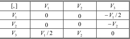
=−V₂, (2f)

where the Lie Brackets satisfy (i) bilinearity, (ii) skew symmetry and (iii) Jacobian identity. For this three-dimensional Lie algebra the commutator Table 1 for V_i is a (3×3)-table whose (i, j)th entry expresses the Lie Bracket

[

V_i,V_j

]

given in (2.f). The table is

skew-symmetric and the diagonal elements vanish.

The coefficient C_i,_j,_k is the coefficient of Vi of the (i, j)thentry of the Table 1 and

the related structure constants can be read from the table to

1 ,

2 1 ,

1 ,

2 1

2 , 2 , 3 1

, 1 , 3 2

, 3 , 2 1

, 3 ,

1 =− C =− C = C =

C . (2g)

Note: It can be shown that the Lie algebra is solvable; to prove this statement see e.g. [2].

Table 1. Commutator Table of the nPDE, eq. (1).

]

[, V₁ V₂ V₃

1

V 0 0 −V1/2

2

V ₀ 0 −V₂

3

V V₁/2 V₂ 0

Other useful algebraic group properties are mentioned: Eq.(1) has no Casimir operator, the group order is three containing seven subgroups.

These subgroups are important to perform a SR later deducing new solutions. The metric (with the symmetric3⊗3second-rank tensor as the Cartanian) satisfies:

  

 

  

  =

4 / 5 0 0

0 0 0

0 0 0

j i

g with det(g)=0 , (2h)

and, since the condition det(g)=0 holds, the given algebra is therefore degenerate.

Alternatively the metric tensor with eq.(2.h) is written as

∑

=

= n

k i

k mi i lk

im c c

g

1 ,

in a

compact form.

Lie symmetries act upon solutions of DEs by mapping the set of solutions to itself. One set is of particular interest those which remain invariant under the action of a Lie symmetry. Given any one-parameter Lie group acting on a DE one is able to find all invariant solutions. If a DE admits an r-parameter Lie group, each of the infinitesimal generators may have associated invariant solutions. Since seven subgroups were found seven different cases by choosing the group constants likely, appear. These cases are listed in Table 2 containing both the transformation for the similarity variable ζ and the similarity function

). (ζ S

Note: Geometrically, a Lie symmetry relates the tangent space of the orbits of points under

the action of the symmetry.

A Lie symmetry is a diffeomorphism, say, it is an invertible function that maps one differentiable manifold to another, such that both the function and its inverse are smooth. A first approach for finding point symmetries (PS) is to make a general change of all variables and then enforce the new variable to satisfy the same set of DEs. This approach leads to complicate nonlinear systems of DEs for the functions used in the transformations. Lie demonstrated that such a procedure is unnecessary.

He established a different method based upon an infinitesimal formulation of the problem for finding the symmetry group of a set of DEs and, replacing these highly complicate equation in the most cases intractable nonlinear equations by tractable linear overdetermined systems of PDEs.

Table 2. Nonlinear similarity transformations for the eq.(1), k_iare the group parameters,

ζand S are the similarity variable and the similarity function, respectively.

Case Choice of the group parameters Transformation for ζ Transformation for S

A k₁ =k₂ =0, k₃ =1 2 =ζ

/x

t u+2lnx=S

B k₁ =k₃ =0, k₂ =1 x=ζ u= S

C k₂ =k₃ =1, k₁ =0 + 2=ζ

/ ) 1

( t x u+2lnx=S

D k₂ =k₃ =0, k₁ =1 t=ζ u=S

E k₁ =k₃ =1, k₂ =0 + 2 =ζ

) 2 ( / x

t u+2ln(x+2)=S

F k₁ =k₂ =1, k₃ =0 t−x=ζ u= S

G k₁ =k₂ =k₃ =1 + + 2 =ζ

) 2 ( / ) 1

(t x u+2ln(x+2)=S

Let us now discuss important similarity solutions for special subgroups. Note that for the Cases A, C, E, and G the following nODE in which the similarity function

) (ζ =S

0 2 ) 6 1 ( 4 2 2

2 _{+ − =}

ζ ζ − − ζ

ζ _eS

d dS d

S d

, S:R×R→R, ζ∈R, −a≤ζ≤a, (3)

where a means an interval upon the real line. Otherwise, for the Cases B and D the nODE arises 0 2 2 = ± ζ S e d S d

, S:R×R→R, ζ∈R, −a≤ζ≤a, (3a)

and finally, for the important case of traveling waves, the Case F is derived to

0 2 2 = − ζ − ζ S e d dS d S d

, S:R×R→R, ζ∈R, −a≤ζ≤a. (3b)

A solution of the nODE eq.(3) is given by (note that ζ=0 and ζ=±∞ are the singular points):

(

)

( ) (

)

                ζ +         ζ π − ζ − ζ ζ +       ζ − − ζ − = ζ ln 2 1 2 4 ln 2 4 1 ; 2 , , 1 , 1 2 4 1 )

( 32 2 1

2

2 e C C erf

F e

S S S , (4)

where C₁ and C₂ are arbitrary constants, the symbolF₂2(.) means a generalized

hypergeometric function and. erf(.) is the error function as usually.

Note: It is not possible to simplify the hypergeometric function in eq.(4); for practical

calculations however, it is useful to introduce a series representation breaking off the second term. The same procedure can be done with the error function to derive a compact form.         ζ − ζ + + ζ + ζ − − ζ ζ − − ζ ζ − =

ζ ( 12) 2 ( 2)ln

12 6 ) 1 ( 4 2 4 1 ) ( 2 2 4 / 1 S S e e e C

S , C=7,37, (5a)

where numerically erf[1/2]≈0,52was used. From this implicit form one calculates the function S(ζ)explicitly. In principle, to handle the solution eq.(4) two ways are suitable: Once by introducing a series representation and otherwise by the help of an integral representation; the function F₂2(.) is expressible in form of a polynomial in the following

form: The general integral representation reads as

t d t x b a F t t a b a b x b b a a

F

∫

a − a b ×

− Γ Γ Γ = − − + − 1 0 1 1 1 1 1 1 2 2 2 2 2 1 2 1 2

2 (1 ) [ , , ]

) ( ) ( ) ( ] ); , ( ), , (

[ 2 2 2 _{, (5b)}

(

)

_       + ζ ζ         ζ + ζ − ζ − =         ζ × − π

∫

4 1

4 1 exp 8 32 1 4 4 , 1 , 1 ) 1 ( 2 2 2 2 4 2 1 0 2 1 1

2 _F t _dt

t . (5c)

Inverting by using both the eq.(4) and the polynomial eq.(5c), one calculates an explicit closed-form representation         ζ − ζ + − + ζ − ζ ζ + ζ − + ζ + ζ − ≈ ζ _{Φ Φ} Φ Φ ln 02 , 0 ) 1 ( 25 , 0 03 , 0 ln 03 , 0 ) 2 2 ( 5 , 0 08 , 0 05 , 0 ln ) ( 5 3 5 3 e e e e S , 2 4 1 ζ =

Φ . (5d)

For large values of the argument, say, ζ →∞, the following formula [8] is employed:

[ ]

[

]

[ ]

[

]

[ ]

[

]

[

1/4

]

[

1

[ ]

]

, exp ) / 1 ( 2 2 2 2 1 ) ( ) ( ) ( ) ( ) ( 1 ) ( ) ( ) ( ) ( ) ( ) ( ) ( 1 ) ( ) ( ) ( ) ( ) ( ) ( ) ( ] ); , ( ), , [( 1 2 3 / 1 4 3 1 2 1 2 1 1 2 2 2 1 1 2 1 2 1 1 1 2 1 1 2 1 2 2 1 2 1 2 1 2 2 2 1 2 2 1 x x b b a a x a x a O O x a a b b O x a b b b a a a b b O x a b a b a a a b b x b b a a F + × = + − Γ Γ Γ Γ + + − − Γ − Γ Γ − Γ Γ Γ + + − − Γ − Γ Γ − Γ Γ Γ = − − + − ζ ζ (5e)

since the first two terms vanish. Note, that the gamma function has poles at x_p =0,−1,−2,....

and for fixed values of the arguments the function F₂2(.) is an entire function of ζ.

The nODE, eq.(3a) allows the following solutions

(

)

(

)

                       − −                 − − = 2 1 1 2 1 2 1 2 sec 2 ln 2 sech 2 ln ) ( C C C C C C S

ζ

ζ

ζ

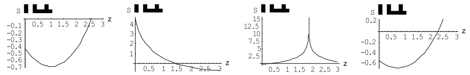
, C₁ ≠0, (6a,b)

where the first solution is valid for a positive sign in the nODE eq.(3a) and the negative sign is related to the second solution. In the Figure 1 and Figure 2 some solution curves are plotted by increasing the domain and a typical periodic run is seen (such solutions are not stable).

The remaining nODE, eq.(3b) admits the following solution

{

C C

}

e

{

D

}

e

S(ζ)= ζ ζ−1+ ₁ + ₂ = ζ ζ−1+ , (7)

where C₁ and C₂ are some non-vanishing arbitrary constants by putting together the

5 10 15 20z 2

4 6 8 10 12

S

H

_z

L

10 20 30 40z 2

4 6 8 10 12

S

H

_z

L

10 20 30 40 50 60z 2

4 6 8 S

H

_z

L

Figure 1. The development of typical periodic behaviour of the solution eq.(6a). Points of

singularities cover point-like diffusion sources. To receive real-valued functions the value of the constant C₁ must taken to be negative then the logarithm function is real. From left to right: C₂ =100, C₂ =60, C₂ =30. The peaks will be crowed together more and more.

0.5 1 1.5 2 2.5 3z

-0.7 -0.6 -0.5 -0.4 -0.3 -0.2 -0.1

S

H

_z

L

0.5 1 1.5 2 2.5 3z 1

2 3 4

S

H

_z

L

0.5 1 1.5 2 2.5 3z 2.5

5 7.5

10 12.5 15

S

H

_z

L

0.5 1 1.5 2 2.5 3z

-0.6 -0.4 -0.2 0.2

S

H

_z

L

Figure 2. Typical solution curves for the solution eq.(6b) where the constant C₁is always

taken to be -1 to ensure that the logarithm function remains real-valued. The constant varies between 1<C₂ <7. The remarkable third sketch represents physically an unit-like diffusion source (analogues to a point-like charge in electrostatics).

Note: Let ζ∈C∞in solution eq.(5). Then the variable ζ may not assume one of the

following forms: ζ_1,2,3,4 ≠1±arcsech

[

±i 2

]

, so regularity is ensured. To be regular further one has to exclude ζ_1,2 =1±4π/3 for the second solution.

2.2 The case of approximate symmetries

In this section the arguments followed in [9], [10] and [11], respectively are considered. The intension is to deduce new results without referring too much theory. The theory of approximate symmetries was developed by Baikov, Gazizov and Ibragimov in the 1980. The idea behind of these developments was the extension of Lie’s Theory for situations in which a small perturbation of the original equations is encountered. For such cases the question arises of how the PS are altered if a small perturbation is added to the original equation.

0 = ε + ∆ − ∂ ∂ u e u t u

. (8)

Thus approximate symmetries follow by the infinitesimals:

(

)

(

)

(

)

(

(

)

)

(

) (

) (

)

(

)

{

}

(

) (

)

(

)

{

(

− +

)

}

ε − − − + + + − + − − − − + + ε + − + + + + + − − − − = φ ε + + + + + = ξ ε + + − + + + − = ξ 2 7 2 7 5 11 5 7 10 1 7 9 2 7 7 7 5 7 1 1 7 9 2 4 12 7 9 6 2 2 4 11 3 7 9 5 8 1 4 4 2 2 2 2 1 4 10 8 4 1 2 4 2 2 1 4 10 8 4 1 2 2 2 2 x u k u k k x u k k x k u k t k u k t k k x t u k x x u k x k k u t k k u k t k k t k k k t t k k k x t k k t k k t x k x k t k k (8a)

representing a twelve-dimensional infinite approximate PS group of first-order approximation depending upon the perturbation parameter. The corresponding twelve generating vector fields are (similarly to the vector fields given in the eq.(2e):

(

) (

)

{

4 4 1 1

}

,

1 =∂ u− u− − u− ε

G _u

{

₄1

(

2 2

)

( )

( )

2

}

,

2 =∂ − tu+ux ε+∂ txε +∂ t ε

G _{u x t} G₃ =ε∂_x,

, 2

4 x x t t

G = ε∂ + ε∂

(

₄1

(

4 4

)

)

2 ,

5 u x x ux t x

G =∂ + − ε − ∂ G₆ =∂_t, G₇ =∂_x, G₈ =ε∂_t,

, 2

9 t x ux u

G =− ε∂ + ε∂ G₁₀ =2t∂_t +x∂_x −

(

2+2ε

)

∂_u,

,

11 u u

G = ε∂ G₁₂ =t2∂_t +tx∂_x + f

(

u,x,t,ε

)

, (8b)

with the function

(

)

(

) (

)

{

− + − + − + + − + − + ε

}

=

ε 2 2

4 1 2 2 2 4

1 _{10 2 2 10 2}

) , , ,

(u x t t tu x ux u t x t tu x ux

f .

To find out approximate similarity solutions one has to combine the vector fields given above. At this stage the coefficients of the vector fields are important and given explicitly by

{

( ) (

0,0 ,(1₄ −4(_u−1

)

+4_u

) (

− _u−1

)

ε

}

,

{

(

_,

) (

_,

(

₂ 2

)

)

}

_, 4

1

2_{ε − − ε}

ε t tu ux

x

t

{

( ) ( )

ε,0, 0

}

,

{

(

xε,2tε

) ( )

, 0

}

,

{

(

−2t,0

)

,

(

x+xε

(

1−u

)

)

}

,

{

( ) ( )

0,1, 0

}

,

{

(

tx,t2

)

,

(

f(u,x,t)

)

ε

}

, (8c)

{

( ) ( )

1,0, 0

}

,

{

(

x,2t

) (

,

(

2 1−ε

)

)

}

,

{

( ) ( )

0,0, uε

}

,

{

(

−2tε,0

) (

, uxε

)

}

,

{

( ) ( )

0,ε, 0

}

.

Note: The main difference between an ordinary vector field vρ of Lie point symmetries and

respect to the perturbation parameter. Thus an approximate vector field is given generally by

(

)

i n

x x x

x

∂ ∂ +

+ +

= ( ) ( ) ... ( )

wρ ξ_i0 εξ_i1 ε ξ_ip . (9)

Possible reductions can be calculated by combining several sub-groups of the eqs.(8b) and (8c); that is G_l ⊗G_m with

{

l,m

}

=1,2,3,...,12. They allow one to investigate new useful approximate symmetry solutions. One is led to Table 3 where some relevant cases are listed.

Table 3. Some special nonlinear transformations in case of approximate symmetries

of eq.(7).

Case Combinations of the vector fields

Transformation for

ζ Transformation for _S

A1 V₃⊗V₄ t/(1−x2)=ζ u=S

B1 V3⊗V6 t−x/ε=ζ u=S

C1 V₃⊗V_{9 t/(x}+ε₎2 =ζ _u+2lnx=S

D1 V3 ⊗V12 t−x=ζ u=S

E1 V₄ ⊗V₉ 2 _=ζ

/x

t u+2lnx=S

The cases A1 and C1 differ by a numerical factor; the derived ODEs are linear and given by Case A1 and Case C1:

0 ) 6 1 (

4 ₂

2

2 ₌

ζ ζ − − ζ ζ

d dS

d S d

and 4 (1 6 ) 2 0

2 2

2 _{+ =}

ζ ζ − − ζ ζ

d dS

d S d

, S:R×R→R, ζ∈R. (10)

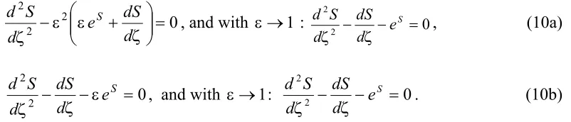
In lowest order perturbation one derives for the Cases B1 and D1:

0 2

2 2

=    

 

ζ + ε ε −

ζ d

dS e d

S

d _S

, and with ε→1 : ₂ 0

2

= − ζ − ζ

S

e d dS d

S d

, (10a)

0 2

2

= ε − ζ − ζ

S

e d dS

d S d

, and with ε→1: ₂ 0

2

= − ζ − ζ

S

e d dS d

S d

. (10b)

0 2 )

6 1 ( 4

2 2

2 _{+ε − =}

ζ ζ − − ζ

ζ S

e d dS

d S d

with ε→1: 4 ₂ (1 6 ) 2 0

2

2 _{+ − =}

ζ ζ − − ζ

ζ S

e d dS d

S d

, (10c)

covering the eq.(3) with known solutions once again. At this stage one still has to propose solutions for the Cases A1 and C1.

Note: The equations for the Cases A1 and C1, respectively are of ordinary and linear type

in which the dependent variable is missed. Procedure: Introduce a function p(ζ)=dS/dζ to

derive the ODE dp/dζ= f(p,ζ). If a solution is known, say,p= p(ζ,c1), the general solution

of Case A1 and/or C1 is found by integration S =

∫

p(ζ,c₁)dζ+c₂.

In addition for the Case A1 a solution is found to

       

ζ π

+ = ζ

2 1 erfc 2

)

( C₁ C₂

S , C₂ ≠0, ζ>0. . (10d)

Further, on the other hand a solution for the Case C1 in a compact form is written by

( )

(

)

_

  

 

ζ − ζ

− ζ −      

ζ π

− = ζ

4 1 ; 2 , , 1 , 1 2

1 ln 2

1 erf 2

)

( 2 3₂

2 2

1 C F

C

S , C₂ ≠0 , ζ>0 , (10e)

where C₁ and C₂ are arbitrary constants. 2(.)

2

F means the generalized hypergeometric

function again and erfc(.) is the incomplementary error function. Note that the occurrence

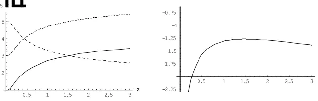
of the error function (also the incomplementary) is a typical sign for diffusion processes as known from literature. In Figure 3 some solution curves are graphically shown.

0.5 1 1.5 2 2.5 3 z 2

3 4 5 S

H

_z

L

0.5 1 1.5 2 2.5 3 -2.25

-1.75 -1.5 -1.25 -1 -0.75

Figure 3. Left: Some solution curves of the eq.(10d), solid line: C₁=1,C₂ =−1, dotted line:

1 ,

3 ₂

1= C =−

C , short dotted line: C₁=5,C₂ =1. Right: Behaviour of the solution eq. (10e), the hypergeometric function is responsible for a small decreasing of the graph.

Note: Due to complexity a closed-form solution neither of the eqs.(3), (3a), (10) and (10b)

solutions. Therefore a solution in the form

∑

=

= n

i i i

a S

0

)

(ζ ζ of the eqs.(10a), (10b) by using a Runge Kutta-like algorithm is derived to obtain

(

)

(

)

(

2

)

...

)

( 3 ₂₄1 2 _{1 1 1}2 4

1 1 6

1 2 1 2

1 1 0

0 0 0

0 0

0

0+ ζ + + + ζ + + + + + ζ +

+ ζ + =

ζ a a a a a a a

e a e a a e e e

a a e a

e a a

S (11)

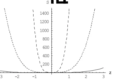
and the coefficients a_i can be chosen arbitrary. In Figure 4 an overview of the polynomial solution by choosing different values of the a_i is seen (questions of convergence should be discussed appropriately).

-3 -2 -1 1 2 3 z 200

400 600 800 1000 1200 1400

S

H

_z

L

Figure 4. The polynomial solution of the eq.(11). Full line:a0 =a1=1, dotted line:

3 1

0 =a =

a , short dotted line:a₀ =a₁=5. By increasing the values of a_i the curves are concentrated around the vertical axes.

2.3. The non-classical case: Generalized symmetries (GS)

It is obvious from Lie theory that PS are a subset of generalized symmetries [12] and [13]. The determination of the characteristics for the general case follows by a similar algorithm as in the case of point transformations (PT) in the classical case. As mentioned classical symmetries of any (n)PDE (generally written ∆=0) are PT which ensures the invariance and so PT are created by infinitesimal transformations. The determining equations for the characteristics Q_α are consequences of the relation

0

0=

∆ υQ _∆=

prρ , (12)

where prυρ_Q denotes the prolongation of the vector field υ_Q. The general expression of the prolongation reads

∑∑

= α ∂ α

∂ =

υ p

n J J

J Q

u Q D pr

1

ρ

where D_J is the total derivative depending upon the multi-index .J The main difference

however is the fact, that, in general the characteristics depend upon derivatives of an infinite order.

If the order is equal to identity one arrives at the so-called contact transformations. By increasing the order of derivatives n>1 one shall find higher order GS. In case of n=1 a GS was found for the nPDE, eq.(1), depending upon the first derivative:

(

x t u u_x u_t

)

k u_x

GS₁ , , , , = ₁ . (14) This symmetry differs from the symmetry given in eq.(2d). Here and in the case above translations appear. The derivative, acting as a slope can be shifted upon an arbitrary plane where the group parameter k₁ can be assumed as a pure real number.

On the other hand eq.(5b) describes an infinite one-parameter translation group whereas eq.(2d) describes an infinite three-dimensional point group. For the case n=2 it was found that GS do not depend upon the first derivative only; the occurrence of second local derivative seems remarkable:

(

)

u

(

)

_{x x}

(

)

_xx

t xx

x u u k e k k t k u k xu k k t u

u u t x

GS₂ , , , , , =2 ₃− ₁+2 ₃ + ₂ + ₃ + ₁+2 ₃ (14a) whereby the character of the symmetry remains the same.

Note: To proceed higher order GS, say, n>2, enormously long calculation time is needed;

a further study is renounced.

2.4. The non-existence of non-classical symmetries

In this paragraph it is shown that the nPDE, eq.(1) does not allow any non-classical symmetries.

Note: The non-classical method of symmetry analysis is an extension of Lie's classical

method. The non-classical method was compiled by Bluman and Cole [14] in connection with the analysis of the heat equation.

This method allows one to derive another type of solutions which are different from solutions derived from Lie's classical procedure. The solutions of the non-classical method will generate a weak symmetry.

Weak symmetries and side conditions were introduced by Olver and Rosenau [15]. On the other hand, it is certain that the vector fields of the non-classical method do not need to form a Lie algebra as in the classical case. Hence there can exist a wider class of similarity solutions than in the classical case.

The tight coupling of the derivatives results into a nonlinear system of determining equations for the infinitesimals. This fact is the main difference between the classical and non-classical method.

However the non-linearity in the determining equations is a real problem in connection with symbolic calculations.

Following the procedure given in [16] a system of nine coupled nonlinear determining equations could derived:

0 2 2 2 2 2 2 2 2 2 1 2 2 ₌ ∂ ∂ ξ ∂ = ∂ ξ ∂ = ∂ ξ ∂ = ∂ ξ ∂ = ∂ ξ ∂ u x x u u

u , (15)

0 2 2 2 2 2 1 2 ₌ ∂ ξ ∂ ξ + ∂ ξ ∂ ξ + ∂ ξ ∂ φ x x

u , (15a)

, 0 2 2 2 3 2 2 2 2 1 2 2 2 2 2 1 2 1 2 2 1 1 2 1 1 2 1 2 2 1 = ∂ ∂ φ ∂ ξ − ∂ ξ ∂ ξ + ∂ ξ ∂ ξ + ∂ ξ ∂ φ ξ + + ∂ ξ ∂ ξ ξ + ∂ ξ ∂ ξ ξ − ∂ ξ ∂ φ ξ + ∂ ξ ∂ ξ − ∂ ξ ∂ u x x x u t x u t u eu (15b) , 0 2 2 2 2 2 2 2 2 2 2 2 1 2 2 2 2 1 2 2 2 2 1 2 1 2 2 2 2 = ∂ φ ∂ ξ − ∂ φ ∂ ξ + ∂ φ ∂ ξ + ∂ ξ ∂ φ ξ − ∂ ξ ∂ ξ + + ∂ ξ ∂ φ ξ − ∂ ξ ∂ φ − ∂ ξ ∂ φ ξ − ∂ ξ ∂ φ ξ + ∂ ξ ∂ ξ + φ ξ x u e t x u x u t x x e e u u u (15c) 0 2 2 2 2 2 1 2 2 1 1 = ∂ φ ∂ ξ + ∂ ∂ ξ ∂ ξ − ∂ ξ ∂ ξ u u x

u . (15d)

The first five equations are linear. One can use these linear equations to find a partial solution of the determining equations. Before the total set of equations is solved one has, for simplification, to rewrite the infinitesimals in such a way that ξ₂ =1 holds. One ends up by four coupled nonlinear determining equations for the infinitesimals: (the index notation for ξ₁ is suppressed, that simply means ξ₁=ξ):

0 2 2 = ∂ ξ ∂

u , (16)

0 2 2 2 3 2 2 2 = ∂ ∂ φ ∂ − ∂ ξ ∂ + ∂ ξ ∂ ξ − ∂ ξ ∂ φ + ∂ ξ ∂ − ∂ ξ ∂ u x x x u t u

eu , (16a)

0 2 2 ₂ 2 = ∂ φ ∂ − ∂ φ ∂ − ∂ φ ∂ + ∂ ξ ∂ φ + ∂ ξ ∂ + φ x u e t x x e

eu u u , (16b)

0 2 2 ₂ 2 = ∂ φ ∂ + ∂ ∂ ξ ∂ − ∂ ξ ∂ ξ u u x

Applying a solving procedure to the system of coupled nonlinear equations eq.(16) to eq.(16c), one automatically can obtain a solution for the infinitesimals. The result is a representation of the non-classical infinitesimals depending upon three arbitrary functionsF_i , i=1,2,3. However the infinitesimal ξ takes an infinite value and can therefore not exist. Analogues to eq.(2.d) one writes

= ξ =

ξ ₁ indeterminate, ξ₂ =1, φ=F₁+u

(

F₂ +uF₃

)

. (17)

3. A

NALYSIS AND

D

ISCUSSION

Due to the similarity of the solutions, especially the eqs.(10d), (10e) and eq.(4) it is convenient to start the analysis by the eq.(10d). By transforming back an expression (in Cartesian coordinates) for the solution eq.(10d) is given through

   

   

− π

=

) 1 ( 2

1 2

) , (

2 x t erfc t

x

u , (18)

where C₁ =0 and C₂ =1 was assumed. This solution correlates to solutions of the linear heat- and/or diffusion equation. It should be regard that the solution eq.(18) is the final result of the approximate symmetry procedure and can therefore be suitable to describe also temperature distributions for different geometries.

Note: Arranging simple boundary conditions, so thatϑ(x,t=0)=ϑ₀=const.holds. Here, ϑ₀is

the temperature at time t=0and furtherϑsis the surface temperature (anisotropic effects

should be excluded and the heat conduction coefficient is equal to unity). Then, from eq.(8)

the temperature distribution follows by =

[ ]

η ϑ

− ϑ

ϑ − ϑ

erfc

s s

0

,

ζ

= η

2

1 _{. Herein it means:}

[ ]

[ ]

_∫

η −

π − = η − = η

0

4 2

1

1 erf e du

erfc u and in addition,ϑ must be bounded as x→∞.

A further property of the error function, that is erfc(x=0)=1,means that the inner part of a material is filled out with heat as t→∞. Generally one may not distinguish between heat and diffusion; essentially a gradient always appears.

For large values of the argument, say x→∞ an asymptotic representation yields

   

 

+ −

+ − π

= − 1 12 120 ...

) , (

6 3

4 2 2

x t x

t x

t

x e t x u

x

, x≠0 (18a)

∑

∞ =

−

π − =

0

1 2

! ) 1 ( ) 0 , (

k

k k

k x x

u . (18b)

A graphical overview both of the solution surfaces is shown in Figure 5

0 1

2 3 x

0 1

2 3

4 5 t 0

1 2 3 u

0 1

2 3 x

1 1.5

2 2.5

3 x

1 1.5

2 2.5

3 t 0

10 20 u

1 1.5

2 2.5

3 x

Figure 5. Representation of the solution surfaces of the solution eq.(18) left and the solution eq.(18a) right.

Finally, for the solution (10e), an asymptotic expression is derived by using the following steps: Consider the divergent series for the error function and x>1

   

 

+ −

+ − π −

= − −

] [ ) 2 (

5 . 3 . 1 ) 2 (

3 . 1 2

1 1 1

)

( 8

3 2 2

2 2

2

x O x

x x

x e x

erf

x

. x≠0. (19)

Then, together with eq.(5e) one derives for the similarity function S(ζ)

π ζ − ζ

− =

ζ ζ −ζ

2 2

3 / 1 4

4 / 6 / 5

) / 1 ( 2 1 )

( e e

S . ζ≠0 . (20)

From the Table 3, Case C1 the transformations u+2lnx=Sand t/x2 =ζ for ε=0are valid.

An analytical solution in conventional form (space/time) is calculated to

x

t x

e

t e x t

x u

x t x

t

ln 2 2

1 ) , (

3 / 1

4 8

4 / 6 / 5 /

2 2 4 2 4

−

      − π −

= − . (20a)

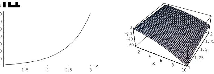
The above given solution can be interpreted as follows: The nonlinear positive exponential term represents a nonlinear propagation of diffusion whereby the negative exponential part represents a kind of nonlinear damping; otherwise the logarithm part counteracts nonlinear diffusion locally.

1.5 2 2.5 3 z

10 20 30 40 50 60 70

S

H

_z

L

2 4

6 8

10 x

1 1.25

1.5 1.75

2

t -60

-40 -20 0

u

2 4

6 8

10 x

Figure 6 Left: The planar plot of the similarity function S(ζ), eq.(20) in the asymptotic

form. Note, that the function is multiplied by (-1). Right: The solution surface u(x,t)of eq.(20a). Both of the cases the initial conditions ζ=0and t=0 lead to singularities. So only time domains with the condition t>0should be considered.

4. C

ONCLUSION

In this study solutions of a highly nPDE with physical relevance are given. The nPDE, eq.(1) can be assumed as a nonlinear extension of the diffusion equation known from literature. Due to the exponential term that makes the linear diffusion equation highly nonlinear, appropriate solution techniques are necessary (no Fouriertransform method is allowed as in the case of the linear heat equation). Therefore to derive analytical solutions the analysis by the classical method of Lie is applied and represents the only viable way of analysis (apart from numerical methods seen as standard procedures and/or functional theoretical methods may generate specific solutions also).

Note: It is proven that algebraic methods such like [17] cannot be applied since the relating

nonlinear algebraic system of equations admits only the trivial solution (the hyperbolic tangent method and its varieties fail).

Otherwise it is shown the following: Introducing the traveling wave reduction in the form u(x,t)→u(ξ), ξ=x−λt in eq.(1) and a transformation u=ln[w(ξ)] lead to the nODE:

0

3 2

2 2

= − ξ λ +      

ξ −

ξ d w

dw w d

dw d

w d

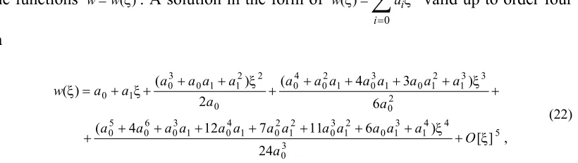
for some functions w=w(ξ). A solution in the form of

∑

=

ξ = ξ

n

i i i

a w

0

)

( valid up to order four

is given

, ] [ 24

) 6

11 7

12 4

(

6

) 3

4 (

2 ) (

) (

5 3

0

4 4 1 3 1 0 2 1 3 0 2 1 2 0 1 4 0 1 3 0 6 0 5 0

2 0

3 3 1 2 1 0 1 3 0 1 2 0 4 0

0 2 2 1 1 0 3 0 1 0

ξ + ξ + +

+ +

+ + + +

+ ξ + +

+ + + ξ + + + ξ + = ξ

O a

a a a a a a a a a a a a a

a

a a a a a a a a a

a a a a a a w

(22)

with suitable chosen coefficients a_i, i=1,2and a₀ ≠0. In Table 4 we summarize some special polynomial solutions depending upon the coefficients. In the Figure 7 some special plane solution curves are shown graphically.

The application of Lie’s method shows that the eq.(1) admits a three-dimensional PS. A suitable choice of the group parameters leads us to invariant solutions containing several special functions for the first time whereby some solutions are of periodic character. A further calculation using approximate symmetries shows that the symmetry behaviour changes to a twelve-dimensional infinite approximate point symmetry group in first-order approximation depending upon a perturbation parameterε≠0.

Table 4. Some special polynomial solutions for the series eq.(22). The first, the fifth

and the last series converges fast.

0

a a₁ Polynomial solution for the function w(ξ),eq.(22)

-3 1 3 3367₆₄₈ 4

27 13 2 6 29

3+ξ+ ξ − ξ − ξ −

-2 -1 3 ₁₉₂7 4

24 37 2 4 5

2−ξ+ ξ + ξ + ξ −

-1 -1 2 ₂₄5 4

2 1

1−ξ− ξ + ξ −

1 -1 3 ₂₄5 4

3 1 2 2 1

1−ξ+ ξ − ξ + ξ −

2 1 3 ₁₉₂617 4

24 59 2 4 11

2+ξ+ ξ + ξ + ξ

3 -2 3 2473₆₄₈ 4

54 125 2 6 25

2

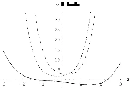
-3 -2 -1 1 2 3 z 5

10 15 20 25 30

w

H

_z

L

Figure 7. Graphical representation of some special solutions of the series solution eq.(22).

Solid line: a₀ =3, a₁ =2, dotted line: a₀ =2, a₁ =1, short dotted line a₀ =1, a₁=−1. In the domain considered the solutions are stable. The functions are even functions and are not periodic.

Different combinations of the vector fields lead to further unknown solutions containing special functions once again (the appearance of the error function is a typical sign for diffusion processes).

Generalized symmetries can be calculated depending upon the derivatives and represents a further new contribution.

It is shown that the eq.(1) does not allow non-classical symmetries since an infinitesimal remain indefinite. Due to complexity several nODEs only could handled numerically in the sense of a Runge-Kutta-like algorithm and the qualitative form of solutions is plotted.

R

EFERENCES

1. H. Fujita, On the nonlinear equations ∆u +exp u =0 and ut = ∆u +exp u. Bull. Amer.

Math. Soc. 75, 1969, 132−135.

2. N. Ibragimov, Lie Group Analysis Of Differential Equations, Vol. III, CRC Press, Inc., Florida, USA, 1994.

3. P. Olver, Applications of Lie Groups to Differential Equations, Springer, New York, 1986.

4. G. Bluman, S. Kumei, Symmetries and Differential Equations, Springer, New York, 1989.

6. A. Huber, A note on class of traveling wave solutions of a non-linear third order system generated by Lie's approach, Chaos Solitons Fractals 32 (4), 2007, 1357−1363.

7. A. Huber, A note on class of solitary and solitary-like solutions of the Tzitzeica-equation,Physica D 237, 2008, 1079−1087.

8. Homepage of the Wolfram Function Site: http://www.wolfram.com, Chapter: Hypergeometric Functions.

9. A. Huber, The Cavalcante-Tenenblat equation –Does the equation admit a physical significance? Appl. Math. Comput. 212, 2009, 14−22.

10. N. Ibragimov, Transformation Groups Applied to Mathematical Physics, Reidel Publ., Dortrecht, 1985.

11. N. Ibragimov, Sophus Lie and harmony in math. physics, On the 150th anniversary of his birth, Math. Intel. 16, 1994, 20−28.

12.E. Noether, Invariant Variation Problems, Transport Theory Stat. Phys. 1, 1971, 186−207.

13.F. Klein, Über die Differentialgesetzte für die Erhaltung von Impuls und Energie in die Einsteinschen Gravitationstheorie, Nachr.d.Kö_{nig. Gesellsch.d. Wiss. zu} Göttingen Math. Phys. Klasse, 1918.

14.G.W. Bluman, J. D. Cole, Similarity Methods for Differential Equations, Springer, New York, 1974.

15.P. Olver, P. Rosenau, The construction of special solutions to partial differential equations, Phys. Let. A 114, 1986, 107–112.

16.P. A. Clarkson, E.L. Mansfield, Algorithms for the nonclassical method of symmetry reductions, SIAM. J. Appl. Math. 54, 1994, 1693−1719.