Int. J. Industrial Mathematics Vol. 4, No. 1 (2012) 41-51
A Method to Estimate the Solution of a Weakly
Singular Non-linear Integro-differential Equations
by Applying the Homotopy Methods
Sh. Sadigh Behzadia∗, A.Yildirimb,c
(a) Department of Mathematics, Central Tehran Branch, Islamic Azad University, Tehran, Iran..
(b)Department of Mathematics, Ege University, 35100 Bornova, I zmir, Turkey.
(c)University of South Florida, Department of Mathematics and Statistics, Tampa, FL 33620-5700.USA.
Received 20 May 2011; Revised 22 October 2011, accepted 29 October 2011.
———————————————————————————————-Abstract
In this paper, the weakly singular nonlinear integro-differential equation is solved by using the homotopy perturbation and homotopy analysis methods . The approximation solution of this equation is calculated in the form of a series which its components are computed easily . The existence and uniqueness of the solution and the convergence of the proposed method are proved. A numerical example is studied to demonstrate the accuracy of the presented method.
Keywords: Volterra integral equations, Integro-differential equations, Singular integral equations, Homotopy analysis method (HAM), Homotopy perturbation method (HPM).
————————————————————————————————–
1
Introduction
Since many physical problems are modeled by integro-differential equations, the numerical solutions of such integro-differential equations have been highly studied by many authors. In recent years some works have been done in order to find the numerical solution of singular integral and integro-differential equations, for example [2, 5, 6, 8, 9, 10, 12, 16,
22, 23, 24]. In this study, we develop HPM and HAM to solve the weakly singular nonlinear Volterra integro-differential equations as follows:
y(k)(x) =f(x) +µ
∫ x
a
1 √
x−t G(y(t)) dt, k≥1, a≤t≤x≤b, (1.1)
with initial conditions
y(r)(a) =br, r = 0,1,2, . . . , k−1, (1.2)
wherea, b, µ, brare constant values,f(x), G(y(t)) are functions which have suitable
deriva-tives on an interval a≤t≤x≤b.
The paper is organized as follows. In section 2, the HPM and HAM are briefly pre-sented. In section 3, these methods are presented for solving Eq.(1.1). Also, the existence and uniqueness of the solution and convergence of the proposed methods are proved. Fi-nally, the numerical examples and computational complexity of the proposed methods are shown in section 4.
To obtain the approximate solution of Eq.(1.1), by integrating k times from Eq.(1.1) with respect tox and using the initial conditions we obtain,
y(x) =F(x) +L−1(
∫ x
a
1 √
x−t G(y(t))dt), (1.3)
whereL−1 is the multiple integration operator as follows:
L−1(.) =
∫ x a ∫ x a . . . ∫ x a
(.)dxdx . . . dx , (k times).
and,
F(x) =f(x) +
k−1
∑
r=0 1
r!(x−a)
rb r.
The following relations have been mentioned in [25]:
L−1(
∫ x
a
1 √
x−t G(y(t))dt) =
1
k!
∫ x
a
(x−t)k√ 1
x−t G(y(t)) dt, (1.4)
so, we can write,
y(x) =F(x) + µ
k!
∫ x
a
(x−t)k√ 1
x−t G(y(t))dt. (1.5)
In Eq.(1.5), we assume that F(x) is bounded for all x inC= [a, b] and
|µ
k!(x−t)
k−12| ≤M′.
Also, we suppose the nonlinear termG(y(t)) is Lipschitz continuous with
|G(y)−G(y∗)| ≤L′|y−y∗|
We set,
2
Introducing homotopy
2.1 Description of the HAM
Let
N[y] = 0,
where N is a nonlinear operator, y(x) is an unknown function and x is an independent variable. If y0(x) denotes an initial guess of the exact solution y(x), h ̸= 0 an auxiliary parameter, H(x) ̸= 0 an auxiliary function, and L an auxiliary linear operator with the property L[r(x)] = 0 when r(x) = 0, then by consideringq ∈ [0,1] as an embedding parameter, we construct a homotopy as follows:
(1−q)L[ϕ(x;q)−y0(x)]−qhH(x)N[ϕ(x;q)] = ˆH[ϕ(x;q);y0(x), H(x), h, q]. (2.6)
It should be emphasized that we have great freedom to choose the initial guessy0(x), the auxiliary linear operatorL, the non-zero auxiliary parameterh, and the auxiliary function
H(x).
Enforcing the homotopy Eq.(2.6) to be zero, i.e.,
ˆ
H[ϕ(x;q);y0(x), H(x), h, q] = 0, (2.7)
we get the zero-order deformation equation as follows:
(1−q)L[ϕ(x;q)−y0(x)] =qhH(x)N[ϕ(x;q)]. (2.8)
When q= 0, the zero-order deformation Eq.(2.8) becomes
ϕ(x; 0) =y0(x), (2.9)
and when q= 1, since h̸= 0 andH(x)̸= 0, the Eq.(2.8) is equivalent to
ϕ(x; 1) =y(x). (2.10)
Thus, according to Eq.(2.9) and Eq.(2.10), as the embedding parameterqincreases from 0 to 1,ϕ(x;q) varies continuously from the initial approximationy0(x) to the exact solution
y(x). Such a kind of continuous variation is called deformation in homotopy [1, 2, 11, 17, 18, 19, 20, 21].
Due to Taylor’s theorem,ϕ(x;q) can be expanded in a power series ofq as follows
ϕ(x;q) =y0(x) +
∞ ∑
m=1
ym(x)qm, (2.11)
where,
ym(x) =
1
m!
∂mϕ(x;q)
Let the initial guess y0(x), the auxiliary linear parameter L, the nonzero auxiliary pa-rameter h and the auxiliary function H(x) be properly chosen so that the power series Eq.(2.11) of ϕ(x;q) converges at q = 1, then, we under these assumptions the solution series is obtained:
y(x) =ϕ(x; 1) =y0(x) +
∞ ∑
m=1
ym(x). (2.12)
From Eq.(2.11) and Eq.(2.8) can be written as follows
L[
∞ ∑
m=1
ym(x) qm]−q L[
∞ ∑
m=1
ym(x)qm] =q h H(x)N[ϕ(x, q)]. (2.13)
By differentiating Eq.(2.13) m times with respect toq, we obtain
m!L[ym(x)−ym−1(x)] =h H(x)m ∂
m−1N[ϕ(x;q)] ∂qm−1 |q=0. Therefore,
L[ym(x)−χmym−1(x)] =hH(x)ℜm(ym−1(x)),
ym(0) = 0,
(2.14)
where,
ℜm(ym−1(x)) = 1 (m−1)!
∂m−1N[ϕ(x;q)]
∂qm−1 |q=0, (2.15)
and
χm=
{
0 m≤1,
1 m >1.
Note that the high-order deformation Eq.(2.14) is governing the linear operator L, and the term ℜm(ym−1(x)) can be expressed simply by Eq.(2.15) for any nonlinear operator
N.
To obtain the approximation solution of Eq.(1.1) based on the HAM let
N[y] =y(x)−L−1(f(x))−∑kr=0−1 r1!(x−a)rbr−µL−1(
∫x a
1
√
x−t G(y(t))dt) = 0.
We obtain the term∑kr=0−1r1!(x−a)rbr from the initial conditions.
We have,
ℜm(ym−1(x)) =ym−1(x)−µL−1
(∫x a
1
√
x−t G(ym−1(t))dt
)
−(1−χm)
(
L−1(f(x)) +∑rk=0−1r1!(x−a)rbr
)
, m≥1.
(2.16)
Substituting Eq.(2.16) into Eq.(2.14),
L[ym(x)−χmym−1(x)] =hH(x)
[
ym−1(x)−µL−1
(∫x a
1
√
x−t G(ym−1(t))dt
)
−(1−χm)
(
L−1(f(x)(x)) +∑kr=0−1 r1!(x−a)rbr
)]
.
We take an initial guess y0(x) = F(x) = L−1(f(x)) +
∑k−1
r=0 r1!(x−a) rb
r, an auxiliary
linear operator Ly=y, a nonzero auxiliary parameter h=−1, and an auxiliary function
H(x) = 1. This is substituted into Eq.(2.17) to give the recurrence relation
y0(x) =L−1(f(x)) +
∑k−1
r=0 r1!(x−a) rb
r,
ym(x) =
∫x a
µ
k!(x−t) k−1
2G(ym−1(t))dt), m≥1.
(2.18)
Relation Eq.(2.18) will enable us to determine the componentsym(x) recursively form≥0.
2.2 Description of the HPM
To explain HPM [3, 4, 7, 13, 14, 15], we consider the following general nonlinear differential equation:
Ly+N y=f(y), (2.19)
with initial conditions
y0(x) =f(x).
According to HPM, we construct a homotopy which satisfies the following relation
H(y, p) =Ly−Lv0+p Lv0+p[N y−f(y)] = 0, (2.20)
where p ∈ [0,1] is an embedding parameter and v0 is an arbitrary initial approximation satisfying the given initial conditions.
In HPM, the solution of Eq.(2.20) is expressed as
y(x) =y0(x) +p y1(x) +p2 y2(x) +· · · (2.21)
Hence the approximate solution of Eq.(2.19) can be expressed as a series of the power of
p, i.e.
y= lim
p→1y=y0+y1+y2+· · ·
we have the recursive relation as follows:
y0(x) =F(x), ..
.
ym(x, t) =
∑m−1 k=1
µ
k!(x−t)
k−12 G(u
m−k−1(t))dt, m≥1.
(2.22)
3
Existence solution and convergence of iterative methods
Proof: Lety and y∗ be two different solutions of Eq.(1.5) then
|y−y∗| =∫ax √µ(x−t)k
x−t k![G(y)−G(y∗)]dt
≤ ∫x a
µ
k!(x−t)
k−12 |G(y)−G(y∗)| dt
≤(b−a) L′M′ |y−y∗|,
Then we obtain (1−α)|y−y∗| ≤0. Since 0< α <1, so |y−y∗|= 0. Therefore, y=y∗
and this completes the proof.
Theorem 3.2. If the series solutiony(x) =∑∞m=0ym(x)obtained from Eq.(2.18) by using
HAM is convergent then it converges to the exact solution of the Eq.(1.1).
Proof: We assume:
b
G(y(t)) =∑∞m=0G(ym(x)), (3.23)
where,
lim
m→∞ym(x) = 0.
We can write
n
∑
m=1
[ym(x)−χmym−1(x)] =y1+ (y2−y1) +· · ·+ (yn−yn−1) =yn(x). (3.24)
Hence, from Eq.(3.23),
lim
n→∞yn(x) = 0. (3.25)
So, using Eq.(3.25)and the definition of the linear operatorL, we have
∞ ∑
m=1
L[ym(x)−χmym−1(x)] =L[
∞ ∑
m=1
[ym(x)−χmym−1(x)]] = 0.
Therefore, from Eq.(2.13) we can obtain that
∞ ∑
m=1
L[ym(x)−χmym−1(x)] =hH(x)
∞ ∑
m=1
ℜm(ym−1(x)) = 0.
Since h̸= 0 andH(x)̸= 0, we have
∞ ∑
m=1
ℜm(ym−1(x)) = 0. (3.26)
By substituting ℜm−1(um−1(x, t)) into the relation Eq.(3.26) and simplifying it , we have
∑∞
m=1ℜm(ym−1(x)) =
∑∞
m=1
[
ym−1−µL−1
(∫x a
1
√
x−t G(ym−1(t))dt
)
−(1−χm)F(x)
]
=y(x)−F(x)−µL−1(∫ax√1
x−t [
∑∞
m=1G(ym−1(t)]
)
.
From Eq.(3.26) and Eq.(3.27), we have
y(x) =F(x) +µL−1(∫ax √1
x−t Gb(y(t)) dt),
therefore,y(x) must be the exact solution of Eq.(1.1).
Theorem 3.3. The series solutiony(x) =∑∞m=0ym(x)obtained from Eq.(2.22) by using
HPM is convergent then it converges to the exact solution of the Eq.(1.1).
Proof: We set,
ϕn(x) =
∑n
i=1yi(x),
ϕn+1(x) =
∑n+1 i=1 yi(x)
so, we have
|ϕn+1(x)−ϕn(x)| =|ϕn+yn−ϕn|
=|yn|
≤∑m−1 k=1 |
µ
k!(x−t)
k−12 ||G(y
m−k−1(t))| dt.
then,
∞ ∑
n=0
∥ϕn+1(x)−ϕn(x)∥≤(m−1)α|F(x)|
∞ ∑
n=0
αn,
Since 0< α <1, therefore,
lim
n→∞yn(x) =y(x).
4
Numerical example
In this section, we compute a numerical example which is solved by the HAM and HPM . The programs have been provided with mathematica 6 according to the following algorithm whereεis a given positive value.
Algorithm: Step 1. n←0.
Step 2. Calculate the recursive relation using Eq.(2.18) for HAM and Eq.(2.22) for HPM. Step 3. If|yn+1−yn|< εthen go to step 4 elsen←n+ 1 and go to step 2.
Step 4. Print y(x) =∑ni=0yi as the approximate of the exact solution.
Lemma 4.1. The computational complexity of the above algorithm for HAM isO(n) and for HPM is O(n2).
HAM: In step 2,
y1 : 5. . .
yn+1 : 5, n≥0.
In step 4, the total number of the computations is equal to∑
n
i=1yi(x, t) = 5n=O(n).
HPM: In step 2,
y1 : 5. . .
yn+1 : 5, n≥0.
In step 4, the total number of the computations is equal to∑
n
i=1yi(x, t) = 4(n−1)n=O(5n2).
Example 4.1. Let us now study the nonlinear singular integro-differential equation as follows
y′′(x) =ex−3.34067×10−16x23 −0.2√x−0.3−1.3333x+
∫ x
0.3 [y(t)]2 √
x−tdt,
with initial conditions y(0) = 1, y′(0) = 1. The exact solution is y(x) =ex, α= 0.98
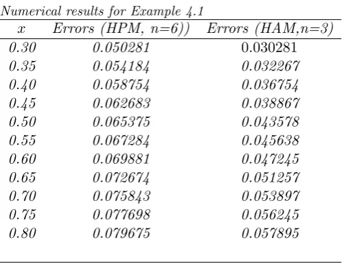
Table 1
Numerical results for Example 4.1
x Errors (HPM, n=6)) Errors (HAM,n=3)
0.30 0.050281 0.030281
0.35 0.054184 0.032267
0.40 0.058754 0.036754
0.45 0.062683 0.038867
0.50 0.065375 0.043578
0.55 0.067284 0.045638
0.60 0.069881 0.047245
0.65 0.072674 0.051257
0.70 0.075843 0.053897
0.75 0.077698 0.056245
Table 1 shows that, the approximation solution of the weakly singular nonlinear Volterra integro-differential equation is convergent with 3 iterations by using the HAM.
5
Conclusion
The HAM has been shown to solve effectively, easily and accurately a large class of non-linear problems with the approximations which converge rapidly to the exact solutions. In this work, the HAM has been successfully employed to obtain the approximate solution to analytical solution of the weakly singular nonlinear integro-differential equation . For this purpose in examples, have shown that the HAM converges more rapidly than the HPM . Also, the number of computations in HAM is less than the number of computations in HPM.
References
[1] A. Adawi, F. Awawdeh, A numerical method for solving linear integral equations. Int. J. Contemp. Math. Science 10 (2009) 485-496.
[2] S. Abbasbandy, Homotopy analysis method for the Kawahara equation. Nonlinear Analysis:Real World Applications 11 (2010) 307-312.
[3] Sh. S.Behzadi, The convergence of homotopy methods for nonlinear Klein-Gordon equation. J.Appl.Math.Informatics 28 (2010) 1227-1237.
[4] Sh.S. Behzadi, M.A. Fariborzi Araghi, Numerical solution for solving Burger’s-Fisher equation by using Iterative Methods. Mathematical and Computational Applications . In Press,2011.
[5] H. Brunner, High-order collocation methods for singular Volterra functional equations of neutral type. Journal Applied Numerical Mathematics 57 (2007) 1-12.
[6] S. Bhattacharya, Numerical solution of a singular integro-differential equation. Ap-plied Mathematics and Computation, 195 (2008) 346-350.
[7] J. Biazar, H. Ghazvini, Convergence of the homotopy perturbation method for partial differential equations. Nonlinear Analysis: Real World Application 10 (2009) 2633-2640.
[8] J.A. Cuminato, A.D. Fitt, S. McKee, A Review of Linear and Nonlinear Cauchy Singular Integral and Integro-Differential Equations Arising in Mechanics. J. Integral Equations Appl. 19 (2007) 163-207.
[10] J.A.Cuminato, A.D. Fitt, M.J.S. Mphaka, A. Nagamine, A singular integro-differential equation model for dryout in LMFBRnboiler tubes. IMA. J. Appl. Math (2005) 1-22.
[11] M.A. Fariborzi Araghi, Sh.S. Behzadi, Numerical solution of nonlinear Volterra-Fredholm integro-differential equations using Homotopy analysis method. Journal of Applied Mathematics and Computing, DOI: 10.1080/00207161003770394, 2010.
[12] M. Ghanbari, M. Askaripour, D. Khezrimotlagh, Numerical Solution of Singular Inte-gral Equations Using Haar wavelet. Australian Journal of Basic and Applied Sciences 12 (2010) 5852-5855.
[13] A. Golbabai , B. Keramati , Solution of non-linear Fredholm integral equations of the first kind using modified homotopy perturbation method. Chaos Solitons and Fractals 5 (2009) 2316-2321.
[14] M. Ghasemi , M. Tavasoli , E. Babolian, Application of He’s homotopy perturbation method of nonlinear integro-differential equation. Appl. Math. Comput. 188 (2007) 538-548.
[15] M. Javidi, A. Golbabai, A numerical solution for solving system of Fredholm integral equations by using homotopy perturbation method. Appl.Math.Comput. 189 (2007) 1921-1928.
[16] M. KOLK, A. PEDAS, Numerical solution of weakly singular Volterra integro-differential equations with change of variables. Proceedings of the 5th WSEAS Int. Conf. on System Science and Simulation in Engineering, Tenerife, Canary Islands, Spain, December 16-18, (2006) 465-470.
[17] S.J. Liao, Beyond Perturbation: Introduction to the Homotopy Analysis Method. Chapman and Hall/CRC Press, Boca Raton, 2003.
[18] S.J. Liao, The proposed homotopy analysis technique for the solution of nonlinear problems. PhD thesis, Shanghai Jiao Tong University, 1992.
[19] S.J. Liao, Beyond perturbation: a review on the basic ideas of the homotopy analysis method and its applications. AdV Mech. 38 (2008) 1-34.
[20] S.J. Liao, On the homotopy analysis method for nonlinear problems. Appl. Math. Comput. 147 (2004) 499-513.
[21] S.J. Liao, Y. Tan, A general approach to obtain series solutions of nonlinear differen-tial equations. Studies in Applied Mathematics 119 (2007) 297-355.
[23] M. Rebelo, T. Diogo , A hybrid collocation method for a nonlinear Volterra inte-gral equation with weakly singular kernel. Journal of Computational and Applied Mathematics 234 (2010) 1-10.
[24] P.S.Theocaris, G. Tsamasphyros, A numerical solution of singular integro-differential equations with vaeiable coefficients. Appl.Math.Comput. 159 (1984) 47-59.