Performance Appraisal of Estimation Algorithms and Application of Estimation Algorithms to Target Tracking

(1)

University of New Orleans University of New Orleans

ScholarWorks@UNO

University of New Orleans Theses and

Dissertations Dissertations and Theses

5-22-2006

Performance Appraisal of Estimation Algorithms and Application

of Estimation Algorithms to Target Tracking

Zhanlue Zhao

University of New Orleans

Follow this and additional works at: https://scholarworks.uno.edu/td

Recommended Citation Recommended Citation

Zhao, Zhanlue, "Performance Appraisal of Estimation Algorithms and Application of Estimation Algorithms to Target Tracking" (2006). University of New Orleans Theses and Dissertations. 394.

https://scholarworks.uno.edu/td/394

This Dissertation is protected by copyright and/or related rights. It has been brought to you by ScholarWorks@UNO with permission from the rights-holder(s). You are free to use this Dissertation in any way that is permitted by the copyright and related rights legislation that applies to your use. For other uses you need to obtain permission from the rights-holder(s) directly, unless additional rights are indicated by a Creative Commons license in the record and/ or on the work itself.

(2)

PERFORMANCE APPRAISAL OF ESTIMATION ALGORITHMS AND APPLICATION OF ESTIMATION ALGORITHMS TO TARGET TRACKING

A Dissertation

Submitted to the Graduate Faculty of the University of New Orleans

in partial fulfillment of the requirements for the degree of

Doctor of Philosophy in

Engineering and Applied Science

by

Zhanlue Zhao

B.S. Xi’an Jiaotong University, China, 1997 M.S. Xi’an Jiaotong University, China, 2000

(3)

c

(4)

(5)

Acknowledgements

I would like to express my deepest gratitude to my major advisor, Dr. X. Rong Li, for

his invaluable inspiration, continuous support, and constructive suggestions, which made it

possible for me to complete the Ph.D. degree. The positive and open research atmosphere

created by Dr. Li is the best nutrition for me to gain considerable knowledge and insights

into problems and techniques in estimation and decision theory, statistical signal processing

and information fusion. The research attitude and enthusiasm exemplified by Dr. Li will

give me everlasting inspiration and encouragement to my future work and research.

I am also indebted to Dr. Huimin Chen. His help, inspiration and encouragement made

my research much more interesting and enjoyable. The collaborations with Dr. Chen often

start with heated discussions and end with insightful ideas. Special thanks go to Dr. Vesselin

Jilkov for the long-term collaboration and his continuous support. I would also thank Dr.

Vesselin Jilkov, Dr. Huimin Chen, Dr. Tumulesh K.S. Solanky, Dr. Zhide Fang and Dr.

Stephen C. Lipp for serving on my thesis committee, and for their constructive and valuable

comments on the dissertation. I am also very grateful to all my friends and members in the

Information and Systems Laboratory, especially Jifeng Ru, Ming Yang, Zhansheng Duan,

Keshu Zhang, Peng Zhang, Anwer Bash, Ryan Pitre, Trang Nguyen and Victor Alvarado.

With their support and friendship, I had the great pleasure of carrying out research in such

a pleasant working environment. And I have to thank many friends who love me and whom

(6)

like to thank all the members and staff of the Department of Electrical Engineering at the

University of New Orleans for their support.

Last but not least, I want to thank my parents for their love and encouragement. Their

(7)

Abstract

This dissertation consists of two parts. The first part deals with the performance appraisal of

estimation algorithms. The second part focuses on the application of estimation algorithms

to target tracking.

Performance appraisal is crucial for understanding, developing and comparing various

estimation algorithms. In particular, with the evolvement of estimation theory and the

increase of problem complexity, performance appraisal is getting more and more challenging

for engineers to make comprehensive conclusions. However, the existing theoretical results

are inadequate for practical reference. The first part of this dissertation is dedicated to

performance measures which includelocal performance measures,global performance

measures and model distortion measure.

The second part focuses on application of the recursive best linear unbiased estimation

(BLUE) or lineae minimum mean square error (LMMSE) estimation to nonlinear

measure-ment problem in target tracking. Kalman filter has been the dominant basis for dynamic

state filtering for several decades. Beyond Kalman filter, a more fundamental basis for the

recursive best linear unbiased filtering has been thoroughly investigated in a series of papers

by Dr. X. Rong Li. Based on the so-called quasi-recursive best linear unbiased filtering

(10)

re-laxed such that a general linear filtering technique for nonlinear systems can be achieved.

An approximate optimal BLUE filter is implemented for nonlinear measurements in target

tracking which outperforms the existing method significantly in terms of accuracy, credibility

(11)

Chapter 1 Introduction

This dissertation consists of two parts. The first part deals with the performance appraisal

of estimation algorithms. The goal is to explore and initiate systematic, comprehensive and

scientifically defensible performance appraisal approaches. The second part is an application

of estimation algorithms to target tracking. The goal is to promote the application of the

recursive best linear unbiased estimation or linear minimum mean square error(LMMSE)

estimation technique. We will apply the recursive best linear unbiased filtering method to

handle nonlinear measurements in target tracking.

1.1 Appraisal of Estimation Performance

The ability to meaningfully assess the performance of an estimation algorithm is crucial for

development and comparison of practical systems. With evolution and proliferation of

esti-mation methods, such as least squares, the method of moments, maximum likelihood method,

Bayes and empirical Bayes procedures, uniformly minimum variance unbiased estimation,

risk-reduction approaches, robust technique and resampling technique, various algorithms

have been developed. In addition, as estimation problems and the related systems of

in-terest are getting more and more complex, huge difficulties are encountered for reconciling

various measures of performance, effectiveness and robustness.

(12)

research focal point sponsored by several agencies of the U.S. Department of Defense. Also,

as pointed out in [58], the emergence of fusion strategies such as adaptive fusion and

fu-sion management requires that Measures of Performance (MoPs), Effectiveness (MoEs), and

Robustness (MoRs) to be examined with greater seriousness. Huge difficulties are

encoun-tered. Further, the optimization of an algorithm with respect to one particular criterion will

frequently result in performance deterioration as measured by another criterion. Because

of this, one might be led to define “global” metrics which measure the overall effectiveness

of an algorithm. One could, for example, try to measure composite algorithm competence

using some ad hoc weighted average of local metrics. In practice, however, such

compos-ite metrics are very difficult to interpret. U.S. Navy investigators on the (Joint Operational

Tactical System) JOTS program concluded after extensive research on practical performance

evaluation techniques that [59]:

“Examination of the host of MoEs as presented earlier does not always provide clear cut

objective distinction of good versus poor performance. During the course of the evaluation,

attempts were made to establish a single MoE as a composite [i.e. weighted sum] of correlator

performance .... several problems were encountered with this MoE, however.... Clearly

a better method of combining MoEs is required .... Such an approach should codify the

philosophy of differing severity of the various types of errors, and nonlinearly increasing cost

associated with those errors as they increase and confusion compounds.”

Therefore, a systematic, comprehensive and scientifically defensible performance

ap-praisal is clearly needed. Towards this goal, we identify important performance aspects

and explore feasible performance appraisal measures. The first part of the dissertation will

be dedicated to theoretical investigations of this topic.

The analysis and comparison of estimation performance have two main aspects.

One is to investigate the properties of estimators and to measure the information

(13)

consistency, credibility and so on [21, 3, 57, 53, 13]. These investigations will provide a profile

of estimation performance which is mainly determined by the formulation of the problem.

For example, the performance bound depends on the likelihood function or the posterior

distribution. The unbiasedness could be either a requirement of problem formulation or a

desired property. These topics have been thoroughly addressed in the subject of statistics.

The other focuses on performance requirements for application purposes or meaningful

interpretation of estimation results. It emphasizes the methods to measure the goodness

of an estimation result relative to the application requirements. In contrast to the former,

existing work dealing with the latter is quite limited, although substantial work has been

done on performance metrics for evaluation of target tracking and data fusion algorithms

[15, 58, 16, 36, 35].

We will focus on the following four topics which are organized as follows.

In Chapter 2, the characteristics of parameter inference are presented. The inherent

gap between estimation problem formulation and application requirements is clarified. A

brief discussion on estimation criteria versus estimation measures is presented. A general

formulation of performance measures is introduced.

In Chapter 3, a group of local performance measures is introduced or proposed. The

pros and cons of most popularly used measures are investigated. New performance measures

are introduced, such as relative error measures, frequency count-type measures and pairwise

comparison measures.

Chapter 4 focuses on global performance measures. In this chapter, the interaction

be-tween estimation criteria and estimator is examined. The performance spectrum is proposed

to reveal such interrelationship. The desired estimation error probability density function

(PDF) is introduced to provide a more comprehensive characterization of the estimation

per-formance requirements. The perper-formance measures relative to the desired PDF is proposed.

(14)

filtering, model approximation is quite common in engineering research and development. It

heavily affects estimation performance. And it is of great interest to have a model distortion

measure to indicate the divergence or difference between the original model and the

approx-imated one. The significance of a model distortion measure is illustrated by its application

to two important problems—model set design and model probability behavior—associated

with the multiple model (MM) algorithm.

The related work on local and global performance measures has been published in [38,

34, 33, 35, 36, 37, 64]. The main results on model distortion measure have been appeared in

[65, 63].

1.2 Application of Estimation Algorithm to Target

Tracking

The second part of the dissertation focuses on the application of the recursive best linear

unbiased estimation (BLUE) to target tracking with nonlinear measurements. The Kalman

filter has been popularly used for state estimation for several decades. Beyond the Kalman

filter, a more fundamental basis is the recursive best linear unbiased filtering which has been

thoroughly investigated in a series of papers by Dr. X. Rong Li [69, 45, 29, 46, 32, 30, 31, 24].

Based on the so-called quasi-recursive best unbiased linear filtering technique, the Kalman

filter’s Linear-Gaussian assumptions can be relaxed such that a general linear filtering

scheme for nonlinear systems could be obtained.

In target tracking, target dynamics is usually modelled in the Cartesian coordinates,

while the measurements are directly available in the original sensor coordinates which are

highly nonlinear with respect to the target state. For a long while, this problem has been

handled by various algorithms based on the Kalman filter but with serious flaws [2, 20, 47,

48, 49, 50, 55, 56]. An approximate BLUE filter is implemented to target tracking with

(15)

accuracy, credibility and robustness without increase in computation. This part is mainly

based on our published papers [67, 66, 68].

In Chapter 6, we present the BLUE filtering technique. Its significance and contribution

are addressed.

In Chapter 7, we apply the BLUE filtering technique to target tracking with nonlinear

measurements. The fundamental flaws of existing measurement conversion methods are

in-vestigated. An approximate implementation of the BLUE filter is presented. The simulation

studies are illustrated. We conclude that the BLUE filter is more fundamental than the

Kalman filter. It outperforms the existing methods significantly.

Chapter 8 concludes the dissertation and provides directions to future work.

1.3 Contributions of the Dissertation

The contributions of this dissertation are summarized as below.

First, a thorough examination of the pros and cons of the most often used local

per-formance measures is conducted. The theoretical and practical justifications and

interpre-tations of these measures are clarified. In particular, the misinterpretation of the most

popularly used root mean square error is elucidated. This part is mainly based on the

papers [38, 34, 33, 35, 36].

Second, we initiate a systematic study for comprehensive and global estimation

per-formance appraisal. A new interpretation of the optimality of the Bayesian estimator is

presented which has a similarity to the lever principle. The interrelationship between the

estimator and estimation criterion is revealed which can help to produce new optimal

esti-mators with predictable estimation performance. Accordingly, an estimation performance

spectrum is proposed for estimation performance comparison. Also, the desired estimation

error probability density function is proposed such that various application concerns and

(16)

esti-mation error distribution relative to the desired one can be measured as well by the proposed

concentration and dispersion measures.

Third, a model distortion measure for statistical inference is proposed to indicate the

model difference between the original model and the approximated one. The distortion

mea-sure turns out to be the Kullback-Leibler divergence. This meamea-sure is highly related to the

behavior of the multiple model algorithm. It can be applied to the model set design problem

for multiple model estimation. Based on the behavior of model probability of the

multi-ple model estimation, the model probability update structure is extended to the multimulti-ple

hypotheses comparison such that an online structure is proposed to carry out the multiple

estimators’ performance comparison and fusion. The illustrative example is demonstrated

as well.

Fourth, we apply the recursive linear minimum mean square error estimation to target

tracking with measurements in polar and spherical coordinates. An approximate LMMSE

fil-ter is achieved which outperforms the existing methods significantly in fil-terms of the accuracy,

(17)

Part I

(18)

Chapter 2 On Estimation Performance Measures

2.1 Parameter Estimation

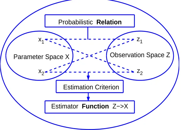
Estimation theory is concerned with inferring the value of a quantity of interest from

indi-rect, inaccurate and uncertain observations. It consists of four components: parameter space,

observation space, probabilistic relation between the parameter space and the observation

space, estimation criteria [57]. The probabilistic relation between parameter space and

ob-servation space determines the formulation of the problem. The parameter is estimated from

observations based on the probabilistic relation, most often, through optimization procedure

with an objective function defined by estimation criterion.

We demonstrate the inference structure by the following diagram.

The complete information on the uncertainty of parameter or state is carried by the

posterior probability density function or likelihood function. For Bayesian estimation, the

prior information of parameter is updated by using observation through Bayesian formula

to obtain the posterior PDF. The estimator is a special point within the domain of the

parameter or state which replaces its posterior PDF with estimation errors. This special

point is determined through optimization procedure. In other words, from a posterior PDF

to an estimator through optimization procedure, we obtain one possible value at the cost of

losing the complete information and producing estimation errors. For classical estimation,

(19)

Parameter Space X x₁

x₂

Observation Space Z z₁

z₂ Probabilistic Relation

Estimation Criterion

Estimator Function Z−>X

Fig. 2.1: Estimation Diagram

function. Usually, the maximum likelihood principle is employed to determine the estimator.

Again, the likelihood function is replaced by a point with associated estimation errors.

For estimation, besides the estimator itself it is also necessary to measure or specify

estimation error in a meaningful and comprehensive manner.

The estimation criterion serves to locate the optimal estimator. It needs to meet two

objectives. First, it should measure the practical requirements adequately. Second, it should

lend itself most easily to manipulation and computation from a technical and mathematical

viewpoint. Most often, an estimation criterion is a compromise of these two objectives and

mainly determined by the second one. It is even more instructive to retrospect the history

of the minimum mean square error (MMSE) as an estimation criterion proposed by Gauss

as follows [17]:

... The integral R∞

−∞x

2_φ₍_x₎_dx_{, i.e., the average value of} _x2_{, seems very suitable for}

defining and measuring, in a general way, the uncertainty of a system of observations.

(20)

agree. The question which concerns us here has something vague about it from its very

nature, and can not be made really precise except by some principle which is arbitrary to a

certain degree.

It is clear to begin with that the loss should not be proportional to the error committed, for

under this hypothesis, since a positive error would be considered as a loss, a negative error

would be considered as a gain; the magnitude of loss ought, on the contrary, to be evaluated

by a function of the error whose value is always positive. Among the infinite number of

functions satisfying this condition, it seems natural to choose the simplest, which is, without

doubt, the square of the error, and is the way proposed above.

Clearly, according to the arguments given by Gauss, the selection of estimation criterion

is arbitrary to a certain degree and can not reflect most of the application concerns. In

order to evaluate the estimation errors or performance for application purposes, we need use

performance measures. We discuss estimation criterion, estimation performance measures

and performance analysis in details next.

2.2 Criteria vs. Measures

Performance optimization, performance evaluation, and performance analysis are closely

related but different. Simply put, performance optimization is based on a theoretical criterion

(objective function); performance evaluation is usually done in terms of some performance

measures; and performance analysis aims at developing a performance model.

Practical measures for performance evaluation of estimation algorithms are closely

re-lated with theoretical criteria for performance optimization. They both should reflect the

performance and fit well with the intended applications. However, they are not to be

con-fused with each other. A performance measure is a ruler/metric that quantifies or sizes up

the performance of the algorithm, while a criterion defines the optimality of the solution

(21)

performance measures that serve as the objective functions for the estimation algorithms to

optimize. As a result, a criterion should be tractable in that it lends itself to easy

mathemat-ical manipulations, rather than merely a meaningful performance measure. In other words,

a criterion formulates the estimation problem as a tractable optimization problem and serves

as the basis for algorithm development. While mathematical tractability is a highly

desir-able property for an optimality criterion—an intractdesir-able criterion is hardly useful—it is not

an important consideration for a performance measure. Compared to estimation criterion,

estimation performance measure only concerns the fitness of an estimator to application

requirements. It can be very complex and comprehensive.

There is also a significant difference between performanceanalysis and performance

eval-uation. Performance analysis focuses on relationships between the performance and its key

factors and hence relies heavily on analytic tools. This is not the case for performance

evalu-ation, which simply evaluates or appraises the performance. Our focal point is performance

evaluation, not performance analysis. Tractability of a performance measure is an important

consideration in performance analysis, but not in performance evaluation, since a highly

com-plex performance measure would most likely render performance analysis intractable, but it

can only make performance evaluation costlier.

2.3 Formulation of Performance Measures

The followingnotational conventionwill be maintained throughout this dissertation. We

refer to any quantity to be estimated as an estimatee. It can be a time-invariant (or slowly

varying) parameter, a (deterministic or random) process or signal, in particular, the state

of a (deterministic or random) system. We will use the term estimator to mean both a

parameter estimator and a filter. The measures are presented in a form suitable for parameter

estimators directly, but are applicable to filters at any given time in a straightforward way.

(22)

˜

x, respectively. They are always assumed to be n-dimensional unless otherwise is stated

explicitly. Subscript i stands for quantities pertaining to the ith run of a Monte-Carlo

simulation. It is always assumed that ˜xi and ˜xj are independent for i 6= j. All default

vectors are column vectors. The Euclidean norm of a vector a is denoted as

ka_k= (a′a)1/2 where a′ _{stands for the transpose of the column vector} _a_.

An estimator is a function of observations which provides a technical guess of a parameter

or state. Since it is data-dependent, its performance is random and should be evaluated in

a statistical sense. In other words, we need to know which estimator is more accurate or

closer to the true value on average than the other. In order to meaningfully quantify such

closeness for comparison purpose, the performance appraisal has to answer the following two

questions:

1. How to quantify the distance between an estimatee and its estimator given each piece

of data?

2. How to measure the performance difference statistically in terms of either marginal

distribution or joint distribution when comparing multiple estimators?

Next, a general formulation of performance measure which incorporates the above two

questions is presented.

First, we give the general performance measure for a single estimator. Define the

perfor-mance measure of a classical estimator as below,

M =Ez[m(x,ˆx)] =

Z

m(x,ˆx)f(z;x)dz

=< m(x,ˆx), f(z;x)>

where parameter x is constant, f(z;x) is the likelihood function of x, m(x,ˆx) is the

measure function of the difference between estimatee x and estimator xˆ, and usually is a

(23)

Similarly, a performance measure of a Bayesian estimator can be defined as

M =Ex,z[m(x,xˆ)]

=

Z Z

m(x,ˆx)f(x,z)dxdz

=

Z

ˆ

M1(z)f(z)dz

=

Z

ˆ

M2(x)f(x)dx

where ˆM1 =

R R

m(x,ˆx)f(x_|z)dxf(z)dz and ˆM1 =

R R

m(x,ˆx)f(z_|x)dzf(x)dx, f(x,z) is

the joint PDF of x and z, again, m(x,ˆx) is the deviation quantification function. Clearly,

the Bayesian estimator’s performance measure M is determined by m(x,ˆx) and f(x,z).

ˆ

M1(z) is the performance measure based on the posterior PDF f(x|z), while z is given;

ˆ

M2(x) is the performance measure based on the likelihood function f(z|x) conditioned on

x.

Second, when comparing multiple estimators, the difference between estimators relative

to the true estimatee can be measured directly. In other words, how often or how much

one estimator is better than the other relative to the true parameter x will be counted.

In this case, the joint distribution information of estimators and estimatee is taken into

consideration [17]. Here, we only stress pairwise comparisons.

The performance measure can be defined for direct pairwise comparison of two classical

estimators relative to the parameter itself as

M(ˆxi:ˆxj;x) =E[m(ˆxi :xˆj;x)]

=

Z

m(ˆxi :xˆj;x)f(z;x)dz

and for direct pairwise comparison of two Bayesian estimators as

M(ˆxi :ˆxj;x) = Ex,z[m(xˆi :ˆxj;x)]

=

Z Z

(24)

where m(ˆxi : ˆxj;x) is the difference between ˆxi and ˆxj relative to the true estimatee x,

i, j _{∈ {}1,2_} and i ₆=j. For example, for pairwise comparison, a meaningful measure could

be Pitman Closeness

m(xˆi :ˆxj;x) =



 

 

1 if ˆxi x

≻xˆj 0.5 if ˆx_i =x ˆx_j 0 if ˆx_i _≺x xˆ_j

where ˆx_i _≻x xˆ_j and xˆ_i _≺x ˆx_j denotes that xˆ_i prefers to ˆx_j and xˆ_j prefers to xˆ_i relative to

x, respectively. If M(ˆxi : ˆxj;x) is larger than 0.5, we say xˆi is better than ˆxj. A detailed

discussion will be given in next chapter.

Usually, the analytical form of performance measures can not be obtained and computer

simulations are resorted to. The use of computer simulations for assessing estimation

per-formance, although quite valuable for gaining insight and motivating conjectures, is hardly

conclusive. Nevertheless, when the performance of some particular scenarios is of interest,

simulation studies can provide a more direct comparison. Therefore, on the one hand,

com-puter simulations are scenario-dependent; on the other, they also give a direct evaluation

under a specific scenario.

When Monte Carlo simulation is employed, all the performance measures simply become

M =E[m(_∗)] = 1

N

X

i=1

ml₍_∗₎

wheremi₍_∗_{) is the measure of the difference between}_x _{and its estimator}_ˆ_x_{or the difference}

between ˆx_i and ˆx_j relative to the true estimatee x, i, j _{∈ {}1,2_}and i₆=j on the lth run of

N Monte Carlo runs.

Local performance measures, global performance measures and model distortion measure

all follow this general formulation. They differ from each other in the specific definitions of

(25)

Chapter 3 Local Performance Measures

This chapter deals with performance measures that are local in the sense that they rely

on relatively local characteristics (e.g., moments) of the distribution of the estimation

er-ror. Interpretation of existing performance measures will be examined and new performance

measures will be proposed. They are classified into the following four categories: absolute

error measures (without a reference), relative error measures (with a reference), frequency

counts (of some events), and pairwise comparison measures. The first three categories are

devised to measure the performance of a single estimator. The last category is for

compar-ison purpose where the joint distribution of the two estimators relative to the parameter is

involved.

This Chapter is organized as follows. In Sec. 3.1, we first discuss several measures of

absolute error of estimation, including the root-mean-square error (RMSE) and what we

called average Euclidean error (AEE). Their pros and cons are presented. It is advocated

that the widely-used RMSE should be replaced by AEE in many applications. Also, two

new measures of absolute error—geometric average error and harmonic average error—are

introduced. Secs. 3.2 and 3.3 are dedicated entirely to new measures. In Sec. 3.2 we

present several measures ofrelative error in that they are normalized estimation errors with

respect to three references, respectively: magnitude of the estimatee, error of prior mean, and

(26)

concentration probability—of an estimation algorithm, which measure how concentrated the

estimates are around the estimatee. They stem from frequency counts of estimates within

some neighborhood of the estimatee, especially within what we called success region and

feasible region. They are complementary to the error measures and are useful for some

applications. Measures for pairwise comparison—Pitman closeness measure, loss measure

and gain measure—are provided in Sec. 3.4. They compare two estimators relative to

the estimatee case by case directly. The performance difference of these two estimators is

concluded by counting on the difference in each case. Illustrative examples are presented in

Sec. 3.5. Sec. 3.6 is concluding remarks.

3.1 Absolute Error Measures

0

3.1.1 RMS Error and Average Euclidean Error

RMSE. By far the most popular measure ofestimation error is theroot-mean-square(RMS)

error, or RMSEfor short, defined by

RMSE(ˆx) =

1

M

XM

i=1kx˜ik 2

1/2

(3.1)

where kx˜ik= (˜xi′x˜i)1/2.

The main nice feature of RMSE is that it is the finite-sample approximation of the

standard error pE[˜x′_x_˜_{], which is closely related with standard deviation. For scalar}_unbiased estimators, it is actually the most natural finite-sample approximation of standard deviation

of estimation error. Since standard deviation is an important parameter for probabilistic

analysis, RMSE is useful for probabilistic analysis in the scalar case. For example, if ˜x

is scalar, zero-mean, and Gaussian distributed with variance σ2_{, then} _P_{|_x_˜_| _< _RMSE_{} ≈}

P{|x˜|< σ}= 0.683.

0 c

[2006] IEEE. Reprinted, with permission, from X. R. Li, Z. L. Zhao, “Evaluation of Estimation

(27)

AEE. An emphasis of this chapter is a proposal to replace in many situations the use of

RMSE with the following average Euclidean error (AEE):

AEE(ˆx) = 1

M

XM

i=1kx˜ik (3.2)

The term “Euclidean error” stems from the concept of Euclidean distance or Euclidean norm.

AEE (in the scalar case) is sometimes called mean absolute error (MAE), but this is not

recommended because the term “absolute error” is ambiguous for a vector. Also, it may

have a misleading implication that it is an absolute error, as opposed to a relative error.

Denote by e = kx˜k the Euclidean norm of the estimation error, which is a random

variable, and let ¯e and σ2

e be the mean and variance of e. Then

E[AEE(ˆx)] = ¯e, var[AEE(ˆx)] =σ_e2/M (3.3) whereσ2

e = var(e) =E(e2)−e¯2 = tr(Σ) +µ′µ−e¯2, and µand Σ are the mean and covariance of estimation error ˜x.

The mean Euclidean error ¯eis clearly a good indicator for the estimation error and, albeit

unknown, it can be estimated. Since AEE and ¯e are respectively the sample average and

the true mean of kx˜k, AEE is the most natural approximation/estimator of ¯e.

RMSE vs. AEE. RMSE and AEE focus on large errors in that their values are

domi-nated by the large error terms. For example, if all 100 terms are around 1 except that one

term is 400, then AEE would be about 5, but RMSE would be approximately 400, that is,

determined by one term while all the other 99 terms are essentially ignored! We say that such

measures are pessimisticsince they pay so much attention to howbad the performance is.

Clearly, RMSE is much more pessimistic than AEE. This example also reveals that RMSE

could be very unreasonable since it is highly distorted—it penalizes too severely on large

errors (i.e., bad behavior) and virtually ignores small errors (i.e., good behavior). This is

highly undesirable or even unacceptable for many applications, particularly as a performance

(28)

the case involving a few huge errors due to, say, filtering divergence: What is the RMSE of

a filter if it diverges on one or few of many runs?

Geometrically speaking, AEE(ˆx) is the arithmetic average of the Euclidean distance

between x and ˆx, while RMSE(ˆx) = √1 M(

PM

i=1kx˜ik2)1/2 is one

√

Mth of the Euclidean

distance between the (M n)-dimensional vectors [x′

1, x′2, . . . , x′M]′ and [ˆx′1,xˆ′2, . . . ,xˆ′M]′, which hardly has a physical interpretation, where xi and ˆxi are the estimatee and estimator on

run i. As such, AEE is truly the average distance between the estimate and the estimatee

in our physical (i.e., Euclidean) space. By contrast, RMSE does not have a simple physical

interpretation—it is not actually an average distance in our Euclidean space, although it is

often so interpreted incorrectly. Clearly, an erroneous interpretation invites confusion and

mistakes.

Consider the case of a scalar measurement z with mean ¯z. Mean deviation E[|z−z¯|] is

no doubt the most natural abstraction of the practical concept of measurement error since

measurement errors in most situations are actually average absolute errors. This should be

clear from the calibration process of a measurement instrument. On the other hand, RMSE

reflects the standard error (or standard deviation pE[(z−z¯)2_{] in the unbiased case). Due}

to the popularity of standard deviation, measurement errors are more often expressed in

terms of RMSE or standard deviation than mean deviation. This is mainly because an

analysis based on the former is more tractable mathematically than on the latter. A

problem in practice is that many practitioners do not understand or are not even aware of

the difference—the former is also interpreted as the average error in magnitude.

The popularity of RMSE arises mostly from the fact that it is in general the best

finite-sample approximation of the standard error, which is the most popular optimality criterion

in terms of error. The widespread use of standard error (in fact, MSE) as a theoretical

criterion is well justified by its mathematical tractability. Such a justification is invalid

(29)

tractability is no longer a concern here. Instead, a clear and correct interpretation of the

metrics is essential.

It follows from the Kolmogorov strong law of large numbers, RMSE2 _{and AEE tend}

(almost surely) to mean-square error E(e2_{) and} _{mean Euclidean error} _e_¯_{, respectively, as}

M → ∞. They are consistent estimators of E(e2_{) and ¯}_e_{, respectively.}

In the scalar Gaussian case, the mean deviation ¯e=E[|x˜|] and the standard deviationσ

are related by E[|x˜|] =σp2/π ≈ 0.8σ. Given an AEE in such a case, it can be converted

to RMSE and thus a probabilistic analysis can still be carried out since such an analysis

almost always assumes a Gaussian error. Note that for the vector case, it is usually not

straightforward to carry out a probabilistic analysis based on RMSE without additional

assumptions, even in the Gaussian case.

It is well known [23] that the conditional mean and median (i.e., the mean and median of

the posterior distribution) minimizes, respectively, MSE and mean Euclidean error and hence

RMSE and AEE. Consequently, the use of RMSE implicitly favors the conditional mean (i.e.,

MMSE) based estimators rather than any other estimator. This is usually a weakness for

performance evaluation, but could be a strength for some other purposes, especially for

verifying that an MMSE-based algorithm is properly designed and/or implemented. By

contrast, AEE favors estimators that minimize mean Euclidean error, which is, however,

rarely used as an optimality criterion due to the difficulty involved.

On the basis of the above arguments, we recommend that RMSE be replaced by AEE

when one is mainly concerned with the magnitude of the estimation errors, since the latter

has a more direct and natural interpretation. When a probabilistic analysis is needed, the

(30)

3.1.2 Harmonic Average Error

As explained before, RMSE and AEE are dominated by their large individual terms and

hence focus on bad behavior. In this sense they are pessimistic measures. However, we may

want to pay more attention to good behavior in some situations, that is, to use optimistic

measures.1 _{For this purpose, we propose the following} _{harmonic average error} ₍_HAE_):

HAE(ˆx) =

1

M

XM

i=1kx˜ik

−1

= M

1/kx˜1k+· · ·+ 1/kx˜Mk

(3.4)

based on the well-known harmonic average. Clearly, HAE is dominated by the small error

terms and hence is an optimistic measure. It focuses on how good (rather than how bad,

as with a pessimistic measure) the performance of an estimator is.

Harmonic average has the following minmax property. Consider the problem of

ap-proximating (estimating) the true error e = _kx˜_k that is bound to be within the

in-terval [a, b]. Denote by ˆe an approximate of e. Then the harmonic average H(a, b)

of a and b yields the minimum of the greatest possible relative error _|e ₋ eˆ_|/e, that

is, H(a, b) = arg mina≤ˆe≤bmaxa≤e≤b(|e − eˆ|/e), while the arithmetic average A(a, b) of

a and b yields the minimum of the greatest possible absolute error, that is, A(a, b) =

arg mina≤ˆe≤bmaxa≤e≤b|e−ˆe| [9].

3.1.3 Geometric Average Error

Neither RMSE and AEE nor HAE is good as abalanced measure for performance evaluation

and, in particular, as a metric for “average” error in magnitude. As far as the average error

in magnitude is concerned, for many problems it is reasonable to expect that any large error

(bad behavior) should be possibly balanced by a sufficiently small error (good behavior) and

vice versa. From this standpoint, the use of the arithmetic average as an average error in

1

(31)

magnitude is flawed. For example, assume AEE is equal to a. Then, an error that is larger

than 2a cannot be balanced by any sufficiently small error. The situation is reversed for

HAE.

In view of the above, we propose the following geometric average error (GAE):

GAE(ˆx) = QM

i=1kx˜ik

1/M

based on the well-known geometric average, which is better

computed recursively

GAEM(ˆx) = GAEM−1(ˆx) [kx˜Mk/GAEM−1(ˆx)]1/M

or through its logarithm for numerical reasons

log[GAE(ˆx)] = 1

M

XM

i=1logkx˜ik (3.5)

GAEM(ˆx) is defined as zero if one or more kx˜ik is zero. Clearly, it does not suffer from the

flaw mentioned above—any large error can be balanced by a sufficiently small error and vice

versa.

Denote by e = kx˜k the random variable that is the Euclidean norm of the estimation

error. It follows from H¨older’s inequality that [18]

¯

e=E[AEE(ˆx)] =E[GAE1(ˆx)]≥E[GAEM(ˆx)]≥E[GAEL(ˆx)]≥GM(e), L > M >1 with all inequalities strict if ¯e < ∞ and GM(e) > 0, where GM(e) = exp[E(lnkx˜k)] is the

geometric mean of the Euclidean norm kx˜k of the random error ˜x in theory. As shown in

[10], ife=kx˜khas zero probability outside the interval [a, b] thenσ2

e/b ≤¯e−GM(e)≤σe2/a, where σ2

e = var(e). Also, by the Kolmogorov strong law of large numbers, GAE(ˆx) tends

(almost surely) to GM(e) as M → ∞. In other words, GAE(ˆx) has an expected value

that converges monotonically to GM(e) from above as the number M of Monte-Carlo runs

increases, and thus it is a consistent, albeit biased, estimator of the geometric mean. In

addition, the application of the central limit theorem to logkx˜1k, . . . ,logkx˜Mk implies that log[GAE(ˆx)] is asymptotically Gaussian (normal) with N(E(logkx˜k),var(logkx˜k)/M) as

(32)

3.2 Relative Error Measures

0

A relative error is one that is relative to some reference. There are many choices for the

reference. Relative error often reveals better the inherent error characteristics of an estimator

than the absolute error. For example, it is usually reasonable to expect that relative error

of an estimator is less variant than the absolute error as the magnitude of the estimatee

varies. Given two estimators and their performance for two different problems, respectively,

it would be misleading to use any absolute error measure for their performance comparison,

but relative error measures can be used. For such reasons, we recommend evaluating the

performance of estimators in terms of a relative error in most cases, although the literature

is full of performance evaluation in terms of absolute error.

Clearly, estimation error ˜xdepends on the magnitude of the estimateexand the accuracy

of the data (measurements)z (as well as the prior distribution ofxfor a Bayesian estimator)

as the input to the estimator ˆx(z). As a result, probably the most natural relative error is

˜

x/_kx_k or _kx˜_k/_kx_k. Another good choice of the reference is the measurement error; that is,

we express the estimation error ˜xin terms of the measurement error. We deal with measures

for such relative errors in this section.

3.2.1 Estimation error relative to estimatee

All the measures discussed in the previous section were given in terms of the absolute error

˜

x. This is often not desirable. For instance, an absolute error of ˜x = 1 is only 1% for an

estimatee of x= 100 but 50% for an estimatee of x= 2.

The relative error ˜x/kxk versions of the measures discussed in the previous section are

simply given by their corresponding formulas with ˜xi replaced by ˜xi/kxik. The absolute

(33)

For example, theRMS relative error (RMSRE) and average relative error (ARE) are

RMSRE(ˆx) =

1 M M X i=1

kx˜ik2/kxik2

1/2

(3.6)

ARE(ˆx) = 1

M

X

i=1

kx˜ik/kxik (3.7)

wherexiis the estimatee on runi(i.e., theith realization of the estimateex). Such measures

are very simple but limited. Relative measures presented below are more appealing.

Improvement of posterior over prior. We now introduce a metric of relative error

for Bayesian (and recursive) estimation. We call itBayesian estimation error quotient

(BEEQ). It quantifies the improvement, in terms of error, of a Bayesian estimator ˆx over

the prior mean ¯x or of the updated estimate ˆx of a recursive estimator over the predicted

estimate ¯x. We define it as

r∗(ˆx) = AEE(ˆx) AEE(¯x) =

PM

i=1kxi−xˆik

PM

i=1kxi−x¯k

(3.8)

where xi and ˆxi are the ith realizations of x and ˆx, respectively, and ¯x is the prior

mean (or prediction) of x. We do not recommend the use of RMSE here, such as

r∗_(ˆ_x_{) =} RMSE∗_(ˆ_x₎

RMSE∗_(¯_x₎ =

PM

i=1kxi−xˆik2/

PM

i=1kxi−x¯k2

1/2

, because of the shortcomings of

the RMSE (e.g., undue dominance of large terms and lack of a natural interpretation) and

the fact that merits of RMSE are largely irrelevant here.

One may be tempted to define BEEQ as _M1 PM

i=1ri, that is, the arithmetic average of individual error quotientsri =kxi−xˆik/kxi−x¯k. This definition is not appropriate. As for

any arithmetic average of a positive quantity, particularly a ratio, the average will be

dom-inated by its large terms (i.e., by the cases in which errors are amplified). In other words,

good (small) terms should be counted but would be essentially ignored in this definition.

What is much worse and in fact fatal is that, as a result of this drawback, this measure is

significantly greater than 1 even for many optimal estimators, which is misleading and

(34)

the geometric average is much more appropriate here and thus BEEQ is better defined as

r(ˆx) = QM

i=1ri

1/M

, which is better computed through its logarithm for numerical reasons:

log[r(ˆx)] = 1

M

X

i=1

logri, ri = k

xi−xˆik

kxi−x¯k

(3.9)

Error amplification and error reduction are thus balanced.

BEEQ quantifies the contribution of the data to Bayesian (and recursive) estimation.

As the error kx−x¯k increases, an approximately constant BEEQ indicates that data has

an insignificant contribution to estimation, because the measurement error is in effect much

larger than kx−x¯k; the degree of drop in BEEQ reflects that of increase in the contribution

of the data; BEEQ will not increase unless an increase inkx−x¯k will lead to an even larger

increase in the measurement error.

It follows from the properties of arithmetic and geometric averages (see, e.g., [9])

that BEEQ is always bounded by the smallest and largest individual error quotients:

rmin ≤ r(ˆx) ≤ rmax, rmin ≤ r∗(ˆx) ≤ rmax, where rmin = min{r1, . . . , rM} and rmax =

max_{r1, . . . , rM}.

3.2.2 Estimation Error Relative to Measurement Error

Clearly, the estimation accuracy depends on the accuracy of the data (measurements) as the

input to the estimator. In fact, a primary benefit of estimation is that estimates are more

accurate than measurements (after they are converted to the same space). As a measure of

this accuracy improvement, we introduce a metric, namedestimate-measurement error

ratio (EMER).

Assume that a (vector-valued) measurementzis related to the estimateexbyz =g(x, v),

where v is the measurement error. Let h(x) =E[g(x, v)_|x] =E[z_|x]. For the additive

zero-mean noise case with z =a(x) +v, we have h(x) = a(x). Then, EMER is defined by

ρ∗(ˆx) = AEE

∗₍_h_(ˆ_x₎₎ AEE∗(z) =

PM

i=1kh(xi)−h(ˆxi)k

PM

i=1kh(xi)−zik

(35)

where AEE∗ _{represents AEE in the measurement space:}

AEE∗(h(ˆx)) = 1

M

X

i=1

kh(xi)−h(ˆxi)k

AEE∗(z) = 1

M

X

i=1

kh(xi)−zik

That is, EMER is defined as—after convertingxand ˆxto the measurement space—the ratio

of the average distance between x and ˆx over the average distance between x and z. Note

that the use of AEE∗ _{is preferable to that of RMSE}∗ _{since RMSE is too much dominated} by the large error terms, although measurement errors are often given in terms of standard

deviation.

Similar to BEEQ, the geometric average of individual estimate-measurement error ratios

is more appealing and thus EMER ρ(ˆx) is better defined by:

log[ρ(ˆx)] = 1

M

X

i=1

logρi, ρi = k

h(xi)−h(ˆxi)k

kh(xi)−zik

(3.11)

Also similar to BEEQ, EMER is always bounded by the smallest and largest individual

error ratios: ρmin ≤ ρ(ˆx) ≤ ρmax, ρmin ≤ ρ∗(ˆx) ≤ ρmax, where ρmin = min{ρ1, . . . , ρM} and

ρmax= max{ρ1, . . . , ρM}.

Clearly, we expect that EMER <1 for a good estimator and the smaller the EMER the

better the estimator.

The ultimate goal of estimation is usually to approximate the estimatee as closely as

possible. The closeness is usually better measured in the estimatee space directly, rather

than in the measurement space, as the above EMER does. In some situations, such as

positioning or localization applications, the mappingh(_·) defined above is invertible; that is,

the mapping h−1₍_·_{) from the measurement space to the estimatee space is known. Then, a}

better definition of EMER is

log[ρx(ˆx)] = 1

M

X

i=1

logρx_i, ρx_i = kxi−xˆik

kxi−h−1(zi)k

(36)

or alternatively

ρ∗_x(ˆx) = AEE(ˆx) AEE(h−1₍_z₎₎ =

PM

i=1kxi−xˆik

PM

i=1kxi−h−1(zi)k

(3.13)

where AEE(h−1₍_z_{)) = AEE(ˆ}_x₎_| ˆ

x=h−1₍_z₎. It quantifies the amount of improvement an estima-tor has on the estimate provided by the measurement directly.

3.3 Frequency Counts of Concentration

0

Simply put, each metric discussed so far provides a ruler to measure how large the estimation

error is: those of Sec. 3.2 are normalized with respect to a variety of references, while those of

Sec. 3.1 are not normalized. In contrast with these error measures, the performance measures

introduced in this section stem from counting the occurrence of some events.

3.3.1 Success Region and Success Rate

Recall that the least-squares (LS) estimation and MMSE estimation differ from the maximum

likelihood (ML) estimation and MAP estimation in their underlying ideas. The former seeks

an estimator that has the smallest error, while the latter uses the “most frequently occurred”

value of the estimatee as the estimator. As such, ML and MAP estimators may have larger

average errors but a higher probability of staying close to the true estimatee. This has

important implications. This fundamental difference should be kept in mind while deciding

on which estimation method to employ for a particular application.

Take the problem of estimation for interception/weapon control as an example. Here what

is important is that the estimates should be within a close neighborhood of the estimatee

(the kill zone of the weapon) such that the target can be destroyed, rather than the average

distance between them. Consider two estimators. The first delivers most estimates within

the kill zone but has some really bad misses. The second misses the kill zone quite often but

has few really bad misses and thus has a smaller average error (squared). Clearly, it is the

(37)

clearly demonstrates another important point: Use of RMSE alone for a comparison between

MMSE (or LS) and MAP (or ML) estimators could be quite unfair, which is unfortunately

quite common in practice. In fact, it should be clear that the use of RMSE to evaluate

estimators for such applications as weapon control and interception is not so appropriate.

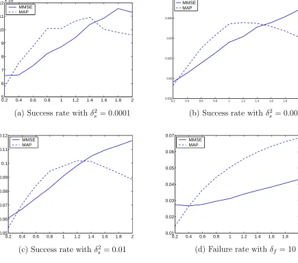
With such applications in mind, we introduce a concept of a success of an estimate and a

corresponding region named success region. An estimator has asuccess given a particular

set of data if its estimate falls inside the success region Rs. Clearly, a good example of a

success region is the kill zone of a weapon, say, a missile—a region in which a target will be

destroyed by the missile. If an estimate is in the success region, a missile detonated at the

location of the estimate will destroy the target, hence a success.

The actual success region is clearly application dependent. We introduce the following

general definition of a success region for the cases when the actual success region is not

known for the application at hand. The success region Rs of an estimator ˆx is a function

of the estimateex and data z defined by

Rs={xˆi :ρi(ˆxi)≤δs} (3.14)

where ρi =kh(xi)−h(ˆxi)k/kh(xi)−zik is the individual estimate-measurement error ratio

(or better use ρx

i = kxi −xˆik/kxi −h−1(zi)k if h(·) is invertible) for some small δs (say,

δs= 0.1). Loosely speaking, for a givenx a success region is a ball kx˜k ≤δskh(x)−zk of a

radius δskh(x)−zk centered at x, meaning that an estimate with an error at mostδs times

the measurement error is treated as a success (e.g., a hit). For a randomx, the center of the

ball is also random.

This definition of success region certainly has drawbacks. For instance, it depends on

data z, while for some applications, e.g., the above interception problem, the success region

should not depend on the data. However, to expect a high success rate of any estimator

based on a set of poor data is unrealistic. This definition is recommended only when the

(38)

The success rate of an estimator is defined as the frequency (percentage) that its

estimates ˆxi are inside the corresponding success region. It is a finite-sample approximation

of the success probability P{xˆ∈Rs}.

3.3.2 Feasible Region and Failure Rate

Similarly, it is also beneficial to introduce the concept of failure for an estimator. We say an

estimator has afailureif its estimate falls outside a region called feasible region. Afeasible

region Rf is one (in the estimatee space) that an estimate falling outside it would result in

a serious consequence—the estimator would usually not be able to recover by itself (due to,

e.g., divergence). For example, in radar tracking, the so-called radar gate is a region (in the

measurement space) in which a target can be tracked in the track mode (rather than the

search mode) of the radar. It can be treated as the feasible region because the target will

be lost if its state estimate falls outside it.

Clearly, the actual feasible region is also application dependent. We introduce the

following general definition of a feasible region for the cases when the actual feasible region

is not known for the application at hand. The feasible region Rf of an estimator ˆx is a

function of the estimatee x and data z defined by

Rf ={xˆi :ρi(ˆxi)≤δf} (3.15)

for some largeδf (say,δf = 10). Loosely speaking, a feasible region is a ballkx˜k ≤δfkh(x)−

zkof a radiusδfkh(x)−zkcentered atx, meaning that an estimate with an equivalent error

in the measurement space greater thanδf times the measurement error is treated as a failure.

Note that the complement (outside) of the feasible region is deemed the failure region.

The failure rate of an estimator is defined as the frequency (percentage) that its

esti-mates ˆxi are outside the corresponding feasible region. It is a finite-sample approximation

(39)

3.3.3 Concentration Region and Probability

The success (or failure) rate is with respect to a specified success (or feasible) region. It

is sometimes more convenient to examine how large the “success” region of an estimator is

given a required success rate. Consider the region

Rδ ={xˆi :ρi(ˆxi)≤δ} (3.16)

If δ > 0 is such that, say, 80% of the estimates fall inside Rδ, then we can refer to Rδ as

the (normalized2_{) 80%} _{concentration region} _{of the estimator and} _δ _{as the 80%} _radius_.

As such, an estimator with a smaller radius δ for a given required success rate (say, 80%)

delivers estimates closer to the estimatee. Given an arbitrary region Rδ, P{xˆ ∈ Rδ} is

the concentration probability of the estimator onRδ. Its finite-sample approximation is

the concentration percentile. Note that although somewhat similar to the concept of a

confidence interval, the concentration region relies on the (individual) estimate-measurement

error ratio.

3.4 Measures for Pairwise Comparison

When two estimators are employed simultaneously for competition, e.g., in a game, their

preference will depend on the pairwise comparison in all cases. In other words, their

perfor-mance difference involves the joint information of these two estimators relative to the truth.

If using measures involves only the marginal information of each estimate, the conclusions

could be misleading. For example when two absolute estimation error sequence are given as

˜

x₁ = [1 2 3] andx˜₂ = [2 3 1], no matter which of the performance measures in Secs. 3.1, 3.2 and 3.3 is used, the difference can not be discriminated. The need for performance measures

for pairwise comparison arises in such situations.

2

(40)

3.4.1 Pitman Closeness Measure

The Pitman closeness measure (PCM) is based on the probabilities of the relative

closeness of competing estimators to the parameter [17]. We explain it next. Letm(ˆx₁ :xˆ₂;x) denote the measure of the difference between ˆx₁ and ˆx₂ relative to the parameter x, and

m(ˆx₁ :ˆx₂;x) =







1 if ˆx₁ _≻xˆ₂ 0.5 if ˆx1 =ˆx2

0 if ˆx1 ≺xˆ2

,

whereˆx₁ _≻xˆ₂means thatˆx₁is preferred toˆx₂relative tox, for example,_||xˆ₁₋x_||<_||xˆ₂₋x_||. The Pitman closeness measure of ˆx₁ superior to ˆx₂ relative to x, is defined as follows

PCM(xˆ₁ :ˆx₂;x) = E[m(ˆx₁ :xˆ₂;x)]

= P r(ˆx1 ≻xˆ2) + 0.5∗P r(ˆx1 =ˆx2)

where E[∗] stands for the expectation of ∗ and P r(∗) is the probability of ∗. Clearly

PCM(ˆx1 :ˆx2;x) = 1−PCM(ˆx1 :ˆx2;x)

When PCM(ˆx1 :ˆx2;x) >0.5 or equivalently PCM(ˆx1 : xˆ2;x) >PCM(ˆx1 : ˆx2;x), we say ˆxi is better thanxˆj. Pitman closeness measure is the relative frequency in which the estimator

ˆ

x1 will be superior to its competitor ˆx2.

PCM is generally applicable and robust against the choice of error measure function.

More specifically, the Pitman closeness always exists; it does not change when different

mea-sures, say theLp _{norms, of the estimation error are used. It uses the joint information of two}

competing estimators, and more information can be extracted. Some peculiar phenomena

about the Pitman closeness have been observed by Rao [17]. He successfully argued for

the Pitman closeness as an intrinsic measure of acceptability and presented many diverse

univariate examples in which shrinking the MSE of an unbiased estimator to an MMSE

esti-mator did not yield a better estiesti-mator in the sense of Pitman closeness [17]. Therefore, the

(41)

not be revealed by MSE. Also, it can discriminate two estimators that are indistinguishable

by measures based on individual information.

However, because PCM is based on the joint information of pairwise estimators, this

invokes some deficiencies [17, 51, 53]. For example, they may take into account a subset of

the sample space that occurs only with probability slightly greater than 0.5; the “winner”

can then be arbitrarily bad when the observation does not belong to this subset. In other

words, they ignore many cases that are still relevant. Due to this peculiarity, they are not

transitive. In other words, ifxˆ1 is better thanˆx2andˆx2is better thanˆx3, according to PCM,

we can not concludeˆx1 is better thanˆx3. Consequently, when more than two estimators are

compared, it might be that none is dominant in the sense of PCM, even though under some

special conditions, the transitiveness does hold. The details can be found in [17, 51].

3.4.2 Loss Measure and Gain Measure

Based on the total probability theorem, a more specified measure with different costs under

conditions of “winning”, “losing” and “even”, respectively, can be defined as below

M(ˆx1 :ˆx2;x) = Pr(ˆx1 ≺xˆ2)E(m(ˆx1 :ˆx2;x)|ˆx1 ≺xˆ2)

+ Pr(ˆx₁ _≻xˆ₂)E(m(ˆx₁ :ˆx₂;x)|ˆx₁ _≻xˆ₂) + Pr(ˆx1 =ˆx2)E(m(ˆx1 :xˆ2;x)|xˆ1 =ˆx2),

where m(xˆ1 : xˆ2;x) is the difference measure between xˆi and ˆxj relative to x, i, j ∈

{1,2}and i6=j, E(m(ˆx1 :xˆ2;x)|ˆx1 ≺ˆx2) is the expectation of m(ˆx1 :xˆ2;x) conditioned on

ˆ

x1 ≺ˆx2. Then , given

m(ˆx1 :ˆx2;x) =

l(x,xˆ₁,ˆx2) if ˆx1 ≺ˆx2

(42)

we have the loss measure (LM) under condition that ˆx1 is inferior to ˆx2 relative to x as

below:

LM(ˆx1 :ˆx2;x) = Pr(ˆx1 ≺ˆx2)E(l(x,ˆx1,ˆx2)|ˆx1 ≺ˆx2),

where l(x,xˆ₁,ˆx2) is the penalty for ˆx1 to be inferior to ˆx2. The smaller LM(ˆx1 : xˆ2;x) is,

the better the estimator ˆx₁ is.

Similarly, thegain measure (GM) thatˆx₁ is superior toxˆ₂ relative to xcan be defined as

GM(xˆ₁ :ˆx₂;x) = Pr(ˆx₁ _≻ˆx₂)E(g(x,ˆx₁,xˆ₂)|ˆx₁ _≻xˆ₂),

where g(x,xˆ₁,ˆx2) is the reward for ˆx1 to be superior to ˆx2. The largerG(ˆx1 :xˆ2;x) is, the

better the estimator xˆ1 is. Obviously, when g(x,xˆ1,ˆx2) ≡ 1, this measure reduces to the

PCM.

The estimators compete against each other case by case directly. The joint information of

the estimators and estimatee is involved, more aspects of the difference between estimators

is revealed.

The loss measure and gain measure can greatly alleviate the peculiarity of the PCM that

“the winner can then be arbitrarily bad when the observation does not belong to this subset”.

Because they still depends on the joint information of estimators, generally speaking, they

are still not transitive.

3.5 Illustrative Examples

Example 1. In this example, we focus on demonstrating that error measures and frequency

counts are complementary.

Given a single linear noisy measurement z of an estimateex:

(43)

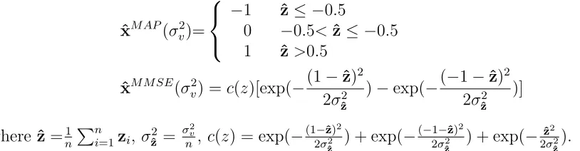
The maximum likelihood (ML) estimator is ˆxML ₌ _z_{. Assume that} _x _{is an exponentially}

distributed random variable with prior pdf f(x) = λe−λx₁₍_x_{), where} ₁₍_x_{) is the unit step} function. It can be shown [23] that two classes of MAP and MMSE estimators, respectively,

with different values of λ, are given by

ˆ

xMAP(λ) = max(z₋λ,0) ˆ

xMMSE(λ) = (√2π[1−Φ(λ−z)])−1e−(z−λ)2/2+z−λ

where Φ(·) is the standard Gaussian cumulative distribution function.

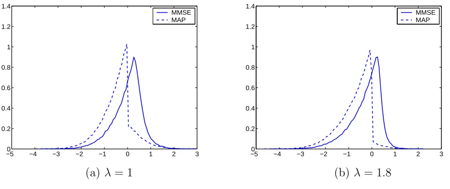
A simulation with 100,000 Monte Carlo runs was conducted in which x was generated

as a random variable with the true density f(x) = e−x₁₍_x_{) (i.e.,} _λ _{= 1). In the following} plots, the x-axis is the λ values assumed in the MAP and MMSE estimators, while the true

λ is always equal to 1.

−50 −4 −3 −2 −1 0 1 2 3 0.2

0.4 0.6 0.8 1 1.2 1.4

MMSE MAP

−50 −4 −3 −2 −1 0 1 2 3 0.2

0.4 0.6 0.8 1 1.2 1.4

MMSE MAP

(a) λ= 1 (b) λ= 1.8

Fig. 3.1: Empirical probability densities of estimation errors of MAP and MMSE estimators.

Fig. 3.1 shows the empirical error pdfs of the MAP and MMSE estimators, each for the

two cases of λ = 1 and 1.8, respectively. Note that the estimation errors of the MAP

estimators are

˜

xMAP=x₋xˆMAP=x₋max(x+v₋λ,0) =

λ₋v z > λ

Performance Appraisal of Estimation Algorithms and Application of Estimation Algorithms to Target Tracking

ScholarWorks@UNO

ScholarWorks@UNO

Performance Appraisal of Estimation Algorithms and Application

Performance Appraisal of Estimation Algorithms and Application

of Estimation Algorithms to Target Tracking

of Estimation Algorithms to Target Tracking

Acknowledgements

Contents

I

Performance Appraisal of Estimation Algorithms

7

II

Application of Best Linear Unbiased Filtering Method to

Target Tracking

83

Abstract

Chapter 1

Introduction

1.1

Appraisal of Estimation Performance

1.2

Application of Estimation Algorithm to Target

Tracking

1.3

Contributions of the Dissertation

Part I

Chapter 2

On Estimation Performance Measures

2.1

Parameter Estimation

2.2

Criteria vs. Measures

2.3

Formulation of Performance Measures

Chapter 3

Local Performance Measures

3.1

Absolute Error Measures

3.1.1

RMS Error and Average Euclidean Error

3.1.2

Harmonic Average Error

3.1.3

Geometric Average Error

3.2

Relative Error Measures

3.2.1

Estimation error relative to estimatee

3.2.2

Estimation Error Relative to Measurement Error

3.3

Frequency Counts of Concentration

3.3.1

Success Region and Success Rate

3.3.2

Feasible Region and Failure Rate

3.3.3

Concentration Region and Probability

3.4

Measures for Pairwise Comparison

3.4.1

Pitman Closeness Measure

3.4.2

Loss Measure and Gain Measure

3.5

Illustrative Examples