journal homepage: http://jac.ut.ac.ir
A Cellular Automaton Based Algorithm for Mobile
Sensor Gathering
S. Saadatmand
∗1, D. Moazzami
†2and A. Moeini
‡31
University of New South Wales, College of Engineering, Department of Computer Science, Sydney, Australia.
2,3University of Tehran, College of Engineering, Faculty of Engineering Science
ABSTRACT ARTICLE INFO
In this paper we proposed a Cellular Automaton based local algorithm to solve the autonomously sensor gath-ering problem in Mobile Wireless Sensor Networks (MWSN). In this problem initially the connected mo-bile sensors deployed in the network and goal is gather all sensors into one location. The sensors decide to move only based on their local information. Cellular Automa-ton (CA) as dynamical systems in which space and time are discrete and rules are local, is proper candidate to simulate and analyze the problem. Using CA presents a better understanding of the problem.
Article history:
Received 20, March 2015 Received in revised form 12, January 2016
Accepted 3, March 2016
Available online 24, March 2016
Keyword: Mobile Wireless Sensor Network Mobile Sensor Gathering Cellular Automata Local Algorithm
AMS subject Classification: Primary 05C80
∗Email:samadseadatmand@yahoo.com †E-mail: dmoazzami@ut.ac.ir
‡E-mail: moeini@ut.ac.ir
1
Introduction
Mobile Wireless Sensor Networks have a wide range of applications and there has been much research on this topic [10]. The mobile sensors have the same general character-istics as in a sensor of a sensor network. A wireless sensor network forms a distributed information processing system that gathers and processes different attributes of the net-work, for example, humidity, temperature, etc [13]. Additionally, each mobile sensor has locomotion capability. One of the main reasons for using the mobile sensors is to improve the coverage of the networks [9].
Normally a large number of sensors are deployed in the environment to sense data and they can disperse to increase the coverage of the network [12]. In an alternative scenario, the sensors need to autonomously move to a single location where they can all communicate with each other directly or where they can be collected for later use. For example, after a certain period of time at the field, the sensors might start losing their energy and want to be back into a position where they can be collected all together.
A set of n mobile sensors are deployed in a wireless network and they are all connected, means that for each sensor there is at least one way to communicate with others and goal is gather all sensors into one location. Please note that in this problem there is no specified destination and the sensors just need to gather to a location. Since each sensor knows only its local neighborhood, it is clear that any successful algorithm for the problem has to maintain connectivity of the network during the intermediate stages of the gathering process [4].
The Cellular Automaton is a biologically inspired model that has been widely used to model different physical systems [7, 2]. We used cellular automata to model the network and algorithm. CA is a discrete time and space model that made of n ≥ 1 dimensional array of cells that each cell in any time step should be in one of its internal states k ≥ 2 [11]. The state of cell c in the next time step determines by local rules based on its current state and current states of neighbor cells [8].
2
Related Works
An analogous problem has been studied in robotics [1, 5] under the name of synchronous gathering problem. A local algorithm proposed in [1] is considerably more complex than our cellular automaton based algorithm. In this algorithm, each sensor determines the smallest enclosing circle that contains all of its neighbors and moves towards the center of that circle. Computing this circle needs a higher number of states compared to our local algorithm. Recently Degener et. al. [5] proved that the running time taken by a sensor
O(n2) is tight. A similar problem is considered for the asynchronous case in [6], where a
In [3], S. Choudhury Introduced a cellular automaton based algorithm. This algorithm is in time O(d2 ∗n) that d is the longest distance between the sensors and the center of network (based on cells) and n is the number of sensors. We introduced an algorithm that is in time O(d). In our algorithm the sensors do not store any previous information and use very limited local information at each time period to find the possible future locations at the next time period. We also show that our algorithm is fast and converges in a finite amount of time and the network remains connected while the sensors move.
3
Proposed Algorithm
Our algorithm used 2-D cellular automaton to model the environment and the sensors. Each cell in CA determines one sensor so that State(c) = 1 for cell cmeans that there is at least one sensor in this cell and State(c) = 0 means that there is no sensor in cell c. The neighborhood radiuses of cells are the communication radiuses of sensors, Rn = Rc
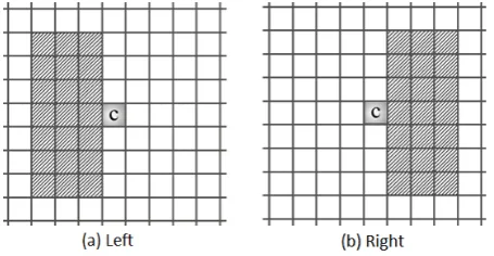
and space is based on the number of cells. Each sensor movement is based on the number of sensors in its neighbor cells and also the sensor can move at most one cell in each time step. We classified the neighbor cells into two main left and right classes (Figure 1) and two axial up and down classes (Figure 2)
Figure 1: Main Classes
Algorithm: For each sensor s in each time step it first checks the main left and right classes as below:
• If it has at least one sensor in its main left and in its main right classes then it doesnt move.
• If it has at least one sensor in its main left class but it hasnt any sensor in its main right class then it moves to its left cell.
• If it has at least one sensor in its main right class and it hasnt any sensor in its main left class then it moves to its right cell.
• If it hasnt any sensor in its main left and in its main right classes then it checks the axial classes up and down classes as below:
– If it has at least one sensor in the axial up class and in the axial down class then it doesnt move.
– If it has at least one sensor in the axial up class and hasnt any sensor in the axial down class then it moves to its up cell.
– If it has at least one sensor in the axial down class and hasnt any sensor in the axial up class then it moves to its down cell.
– If it hasnt any sensor in the axial up and down classes then the end of algorithm .
Briefly each sensor that is in the left or right border of network will moves inside hor-izontally. The sensors that are in the left and right borders (they havent any neighbor sensors in their main left and right classes), will move inside vertically.
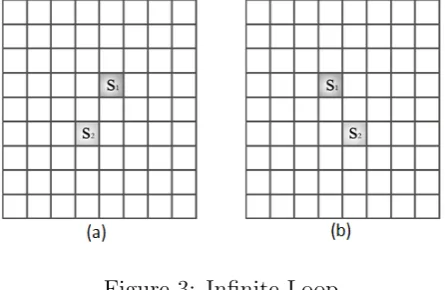
Infinite loop: In Figure 3(a) sensors1 is in the right border and sensor s2 is in the left
border. So in each time step sensor s1 will moves to its left cell and sensors2 will moves
to its right cell and Figure 3(b) will be appears, and repeat these two phases will cause an infinite loop.
To prevent these infinite loops we put the movement priority on left border sensors. It means that only sensor s2 in Figure 3(a) will moves to its right cell. To implement this,
each cell has a flag that initially is 0. Each time the left border sensor decides to move to its right cell, it first set its and its axial up and down cells flag to 1. Each sensor in the right border, before moving, will check the flag of cells in its left column. If there is at least one cell that has flag 1, it doesnt move. With assumptionRc= 2 the neighbor cells
of sensors2 that should have flag 1, are shown in Figure 4 (flag of sensors2 is 1 too). The
Figure 3: Infinite Loop
Figure 4: Neighbor cells with flag 1
Theorem All sensors gather into a cell in a O(d) time where d is the longest distance between any given sensor and the center of network (approximately half of the network diameter).
Proof At each time step, all sensors that are in the left or right borders will move to the inside of network horizontally, and all sensors that are in the left and right borders will move to the inside of network vertically. Suppose that shape is the form of sensors deployment in the network. Assume three cases best, average and worst:
• Best case Shapeis square (or circle) and the sensors deployed densely, means that there is no additional empty cell between each two sensors. Sod will be about √n. All sensors after d/2 iterations will gather into a vertical line and then after other
d/2 iterations they will gather to a single cell. So the algorithm will finishes afterd
iterations and algorithm is in timeO(d) = O(√n).
• Average case Shape is square (or circle) and there are Rc cells between each two
sensors. So d will be about Rc∗
√
n. All sensors after d/2 iterations will gather into a vertical line and then after other d/2 iterations all sensors will gather to a single cell. So the algorithm will finishes after d iterations and algorithm is in
O(d) =O(Rc∗
√
• Worst caseAll sensors are in a line and there areRccells between each two sensors,
sod will be Rc∗n. In this case algorithm will finish afterd/2 iterations because in
each time step border sensors will move one cell toward the center of the line. So in this case algorithm is in O(d) =O(Rc∗n).
So in all cases algorithm is inO(d) and the d can change between √n up to Rc∗n.
Theorem Algorithm never breaks the connectivity.
Proof At any given time stept, if the network is connected then at timet+1, it will also be connected, because each border sensor always moves away from the border and moves toward the inside of network and there is no possibility of breaking connectivity.
References
[1] H. Ando, I. Suzuki, and M. Yamashita. Formation and agreement problems for syn-chronous mobile robots with limited visibility. In Proceedings of the 1995 IEEE Inter-national Symposium on Intelligent Control, pages 453-460. IEEE, Aug 1995.
[2] P.P. Chaudhuri. Additive cellular automata: theory and applications. IEEE Computer Society Press, 1997.
[3] S. Choudhury, Cellular automaton based algorithms for wireless sensor networks. Ph.D thesis, School of Computing, Queens University, ON, Canada 2012
[4] S. Choudhury, S. G. Akl, and K. Salomaa. Cellular automaton based motion planning algorithms for mobile sensor networks. In To appear in Proceeding of the First Interna-tional Conference on the Theory and Practice of Natura Computing, Tarragona, Spain, October, 2012.
[5] B. Degener, B. Kempkes, T. Langner, F. Meyer auf der Heide, P. Pietrzyk, and R. Wattenhofer. A tight runtime bound for synchronous gathering of autonomous robots with limited visibility. In Proceedings of the 23rd ACM symposium on Parallelism in algorithms and architectures, SPAA ’11, pages 139-148. ACM, 2011.
[6] P. Flocchini, G. Prencipe, N. Santoro, and P. Widmayer. Gathering of asynchronous robots with limited visibility. Theoretical Computer Science, 337(1-3):147-168, 2005.
[7] M. Garzon. Models of massive parallelism, Analysis of cellular automata and neural networks. Texts in Theoretical Computer Science, Springer-Verlag, 1995.
[9] B. Liu, P. Brass, O. Dousse, P. Nain, and D. Towsley. Mobility improves coverage of sensor networks. In Proceedings of the 6th ACM international symposium on Mobile ad hoc networking and computing, MobiHoc ’05, pages 300-308. ACM, 2005.
[10] X. Li. Improving area coverage by mobile sensor networks. Ph.D. thesis, SCS, Carleton University, ON, Canada, 2008.
[11] J.L Schiff. Cellular automata: a discrete view of the world. Willey series in discrete mathematics and optimization, University of Auckland, 2008.
[12] S. Torbey. Towards a framework for intuitive programming of cellular automata. M.Sc thesis, School of Computing, Queens University, ON, Canada, 2007.