Software for Estimation of Human Transcriptome Isoform Expression Using RNA-Seq Data

(1)

University of New Orleans University of New Orleans

ScholarWorks@UNO

University of New Orleans Theses and

Dissertations Dissertations and Theses

Spring 5-18-2012

Software for Estimation of Human Transcriptome Isoform

Expression Using RNA-Seq Data

Kristen Johnson

Follow this and additional works at: https://scholarworks.uno.edu/td

Part of the Numerical Analysis and Scientific Computing Commons, and the Other Computer Sciences Commons

Recommended Citation Recommended Citation

Johnson, Kristen, "Software for Estimation of Human Transcriptome Isoform Expression Using RNA-Seq Data" (2012). University of New Orleans Theses and Dissertations. 1448.

https://scholarworks.uno.edu/td/1448

This Thesis is protected by copyright and/or related rights. It has been brought to you by ScholarWorks@UNO with permission from the rights-holder(s). You are free to use this Thesis in any way that is permitted by the copyright and related rights legislation that applies to your use. For other uses you need to obtain permission from the rights-holder(s) directly, unless additional rights are indicated by a Creative Commons license in the record and/or on the work itself.

(2)

Software for Estimation of Human Transcriptome Isoform Expression Using RNA-Seq Data

A Thesis

Submitted to the Graduate Faculty of the University of New Orleans

in partial fulfillment of the requirements for the degree of

Master of Science in

Computer Science

by

Kristen Johnson

B.S. University of New Orleans, 2007

(3)

(4)

Acknowledgments

I would like to thank my professors for all the knowledge they have passed on to me

since I began my studies in Computer Science. Most importantly I give special thanks to my

advisor, Dr. Dongxiao Zhu, for sharing his knowledge of bioinformatics as well as his support

and advice throughout the course of my graduate studies and research. Dr. Zhiyu Zhao, who got

me started in bioinformatics research and who I have enjoyed working with since. Dr.

Christopher Summa, for his endless advice and good humor. And finally, Dr. Jaime Nino, for

teaching me everything about programming I needed to know, just as he promised.

I would also like to thank everyone in our Bioinformatics group, especially Nan Deng.

Nan taught me everything she knew about this topic and helped make this thesis possible. I wish

to thank her for her patience with answering my endless questions.

Finally, I would like to thank my family and friends who have always supported me. My

love and gratitude go to my mom and siblings for keeping me focused and understanding why I

am always busy, my aunt Kyle for getting me back on my feet, and my best friends Sancy and

Jeff for keeping me there. I would also like to thank my boyfriend, Brendan, for never getting

tired of me picking his brain, always making me laugh, and making me as confident as he is by

always supporting me. Lastly I wish to thank my grandmother, quite possibly the most important

person I have had in my life so far, for being my guide, best friend, and inspiration to stay strong

(5)

List of Figures

Figure 1. Central Dogma of Molecular Biology and Alternative Splicing ...5

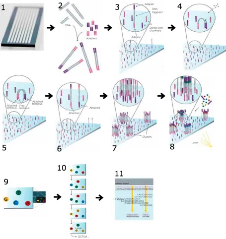
Figure 2. RNA-Seq Workflow Illustrated Using Illumina Sequencer ...9

Figure 3. UML Diagrams of Classes Gene, mRNA, and Exon ...30

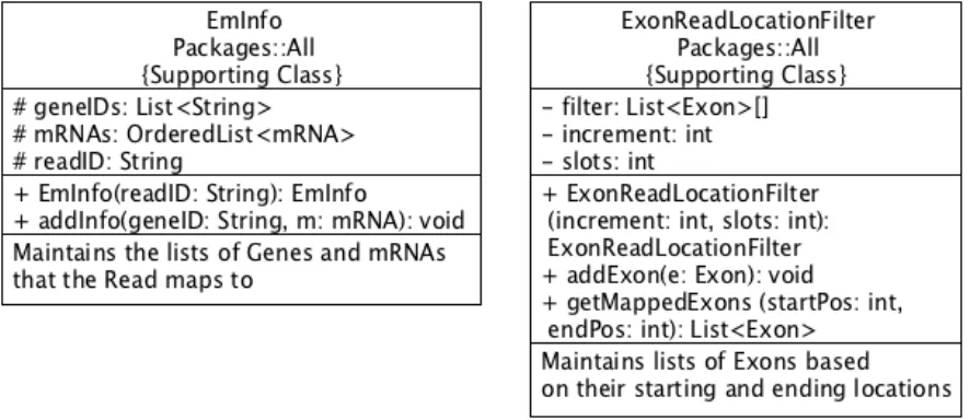
Figure 4. UML Diagrams of Classes EmInfo and ExonReadLocationFilter ...32

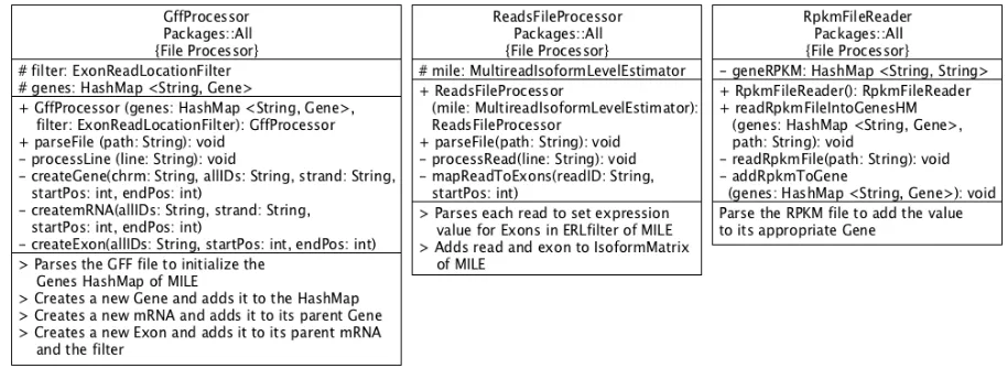
Figure 5. UML Diagrams of File Processing Classes ...35

Figure 6. UML Diagrams of MILE ...36

Figure 7. E and M Steps of GWIE and ChromIE ...40

Figure 8. iGWIE Intermediate Results ...45

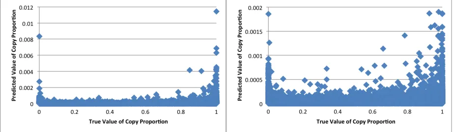
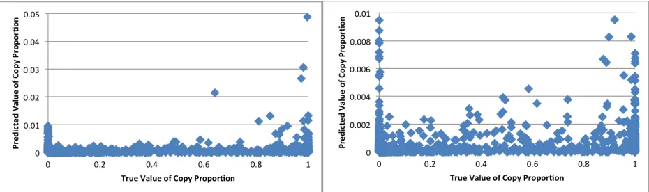
Figure 9. iGWIE Predicted Copy Proportions vs. Real Copy Proportions ...45

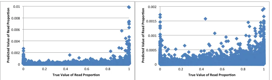
Figure 10. iGWIE Predicted Read Proportions vs. Real Read Proportions ...46

Figure 11. ChromIE Analysis of Chromosome X ...47

Figure 12. ChromIE Predicted Copy Proportions vs. Real Copy Proportions ...47

Figure 13. ChromIE Predicted Read Proportions vs. Real Read Proportions ...48

(8)

Abstract

The goal of this thesis research was to develop software to be used with RNA-Seq data

for transcriptome quantification that was capable of handling multireads and quantifying

isoforms on a more global level. Current software available for these purposes uses various

forms of parameter alteration in order to work with multireads. Many still analyze isoforms per

gene or per researcher determined clusters as well. By doing so, the effects of multireads are

diminished or possibly wrongly represented. To address this issue, two programs, GWIE and

ChromIE, were developed based on a simple iterative EM-like algorithm with no parameter

manipulation. These programs are used to produce accurate isoform expression levels.

Keywords

RNA-Seq

Transcriptome Quantification

Isoform Expression

(9)

Chapter 1: Introduction

1.1: Motivation

Estimation of gene expression levels from RNA-Seq data can be achieved with greater

accuracy through estimation of the transcript abundance of each gene. This estimation is a useful

biological tool for understanding transcriptional regulation and gene functionality. Increasing

understanding of the transcriptome is important for determining the characteristics of both

normal development in cells, as well as the progression of various diseases [2, 38].

As a result of the use of high-throughput, next-generation sequencing technologies, most

notably RNA-Seq, data can be obtained that provides a more absolute coverage of transcript

levels than previous microarray technologies. However, due to the size and complexity of this

data, programs must be designed to aid biomedical researchers in its interpretation. The large

amount of data produced by RNA-Seq is a typical problem faced by bioinformatics researchers.

Efficient methods for storage, retrieval, and processing must be designed to further research in

this field [38, 39, 40].

The software designed for this thesis presents a simple command line interface that

merely requires the input paths for three files. From this, it will perform direct isoform

expression calculation without the need for confusing parameter setting or understanding, as is

common with many popular bioinformatics software tools. Despite the drawbacks of

computational time due to large input data files, the trend towards faster, more powerful

computers supports that this approach can be useful because of its simplicity and accuracy.

1.2: Objectives

The initial objective of this thesis was to extend the work previously done in [8] to design

(10)

considered during the estimation. Separate reads are those reads that map only to one gene,

meaning multiple mappings were discarded from the calculation.

An additional goal was to broaden the level of analysis from a gene based level to a more

global level in order to obtain a more accurate analysis of all isoforms simultaneously.

Previously, only the isoforms of each gene are compared to each other. This ignores the

statistical contribution of multiple mappings to multiple genes.

1.3: Contributions

The main contributions of this thesis are the achievement of the stated objectives. In

order to achieve these goals, two programs were designed and implemented using the

programming language Java. Both programs consider all reads, not just separate reads during the

isoform expression estimation. Each program achieves estimation at a more general, global level

than the gene based approach in [8].

Genome Wide Isoform Estimation (GWIE) was designed to include all reads and to

analyze them at the global level. This means that all reads are assigned to the isoforms that they

could possibly belong to, which could fall under multiple genes. During the estimation, over

90,000 isoforms of all genes are compared using the EM algorithm.

Chromosomal Isoform Estimation (ChromIE) was designed with the hope to achieve

faster results than GWIE, while incorporating all reads but analyzing them per chromosome.

This achieves multiple read mapping inclusion and estimation at a level higher than the gene

based approach in [8]. However, in this exchange for quicker result production, ChromIE is not

as global as the genome wide approach of GWIE. For example, while computing the estimated

(11)

831,053 short reads to these isoforms. For chromosome one, ChromIE compares 11,215

expressed isoforms with 1,900,016 short reads.

In addition to these software based contributions, additional work was contributed to two

publications. For [8], test programs were implemented and used for results verification. Other

party software was run to further support the findings of [8] to fulfill reviewer revision

suggestions before publication. For [43] the de novo transcriptome assemblers, SPATA and

Trans-ABySS, were run using both human and mouse data in order to analyze performance and

accuracy.

1.4: Overview

This thesis is organized into six chapters. Chapter one consists of a brief introduction and

the objectives, motivation, and contributions behind this work. Chapter two consists of a

discussion of the background information necessary for understanding why the software was

designed for this thesis. Chapter three covers software that computes isoform expression levels

like the software of this thesis. Chapter four describes in detail the software designed for

achieving the goals of this thesis. Chapter five discusses the intermediate results of the two

(12)

Chapter 2: Background Information

2.1: Genome and Transcriptome

The genome of an organism constitutes all of the biological information needed to build

and maintain that organism. This biological information is represented through deoxyribonucleic

acid (DNA), which is further segmented into chromosomes. These chromosomes can further be

divided into multiple genes. These genes carry the instructions necessary for producing

ribonucleic acid (RNA) or protein molecules [1, 3]. For the purposes of this thesis, chromosomes

one through twenty-two, X, and Y are considered but only the protein coding genes of these

chromosomes, 21,280 in total, are evaluated [9].

The transcriptome refers to the set and amount of all transcripts, which include all forms

of RNA molecules, in a cell at a given time. This time could be during a stage of normal

development or a certain condition, such as disease. This leads to the biological importance of

understanding the transcriptome in order to determine the progression of both normal

development and diseases and is particularly useful in the study of cancer [1, 8, 39, 40]. This

thesis evaluates the expression of only 100,298 possible mRNAs [9].

2.2: Central Dogma of Molecular Biology

According to the central dogma of molecular biology, DNA encodes for RNA, which

encodes for protein. Though there are special cases, such as RNA encoding for RNA, of most

importance to the study of the transcriptome is the flow of information from DNA to RNA [6].

Transcription is the transference of DNA information to a messenger RNA (mRNA) molecule.

For eukaryotic cells, a primary transcript called pre-mRNA undergoes further processing, such as

(13)

dogma [16]. The thesis software aims to evaluate the expression levels of these transcripts in

order to determine which isoforms of which genes are most highly expressed at a given time

within a cell, or within a certain type of tissue sample. Figure 1 below shows the flow of genetic

information through both the central dogma and alternative splicing.

Figure 1. Central Dogma of Molecular Biology and Alternative Splicing. The flow of genetic information via the central dogma can be seen via the arrows. DNA is transcribed into pre-mRNA which undergoes alternative splicing to produce pre-mRNA. Different isoforms of pre-mRNA are translated into different proteins. This figure was modified from [2].

2.3: Alternative Splicing

While the genome is more fixed, with the exception of mutations, the transcriptome is

highly variable, dynamic, and dependent on external environmental conditions, such as tissue

types. Alternative splicing is considered a key factor in the cause of the transcriptome, cellular,

(14)

first-generation sequencing techniques, the extent of alternative splicing found in humans was not

fully explored until the advent of next-generation sequencers [24, 26, 40].

Transcripts undergo processing via splicing to remove introns. This is done as the

precursory step to creation of messenger RNA (mRNA) molecules, which only contain exons.

Alternative splicing not only increases the range of the transcriptome, but also produces multiple

transcripts from a single gene because of the splicing variants produced due to inclusion or

exclusion of exons, as can be seen in Figure 1 [40].

2.4: Next-Generation Sequencing

Next-generation sequencers can generate over tens of millions of short reads per

experiment. These short reads are generated from a library of nucleotide sequences and are

commonly referred to as the high-throughput data output by next-generation sequencers. The

produced reads can range in length, from as short as 25 base pairs (bp) to as long as 200 bp [21,

23, 24, 30].

Prior to next-generation technologies, methods that used microarrays, Sanger sequencing,

serial analysis gene expression (SAGE), or cap analysis gene expression (CAGE) were used to

determine full-length cDNA sequences. Use of Sanger sequencing based methods dominated

DNA sequencing for over three decades. However, through the effort to understand the human

genome, it was realized that greater throughput was necessary. Around 2004 to 2005,

development of inexpensive, non-Sanger based sequencing technologies by 454 Life Sciences

and the lab of George Church began a sequencing revolution. Despite initial negative attitudes

towards aspects such as sequencing validity, read length, and manageability of the volume of

(15)

most Sanger based technologies suffered similar problems during their initial development [21,

23, 30].

The most commonly used next-generation sequencers of today include the Illumina

Genome Analyzer, HiSeq (Illumina/Solexa), Applied Biosystems’ Solid Sequencing (SOLiD),

and Roche/Life Sciences’ 454 Sequencing (454 Sequencing). These different platforms acquire

the same information and can be applied in similar or different research areas. For instance,

Illumina has been used recently for sequencing mammalian transcriptomes. SOLiD has been

used for profiling stem cell transcriptomes. While 454 sequencing has been used to discover

single nucleotide polymorphisms (SNPs) in corn [21, 23, 30].

Each approach employs a different sequencing chemistry. Illumina uses polymerase

based sequence-by-synthesis, SOLiD uses ligation based sequencing, and 454 Sequencing uses

pyrosequencing. The parallelized version of pyrosequencing used by 454 Sequencing uses

emulsion PCR in combination with detection of added nucleotides to nascent DNA via light

generated by luciferase to generate reads. Illumina’s detection is based on the combination of

bridge amplification and reversible dye-terminators. SOLiD uses emulsion PCR prior to

sequencing by annealing and ligation of oligonucleotides [21, 23, 30].

Each sequencer has varying performance rates for paired end separation, mb per run, read

length, running time, and cost. 454 is the fastest, taking only several hours, and cheapest for cost

per run, but most expensive for cost per mb. SOLiD takes approximately five days to sequence

paired end data and is the most expensive. Illumina can take between one to two weeks and is

more expensive than 454 Sequencing but less expensive than SOLiD. Though these three

sequencers remain the most popular and widely used currently, several other next-generation

(16)

2.5: RNA-Seq Technology

RNA-Seq technology is the use of high-throughput data produced by the next generation

sequencing technologies (as described in section 2.4) to classify the transcriptome of individual

cells, specific tissues, or entire organisms [23]. Next-generation tools provide excellent genome

coverage and base level resolution, which allows for efficient measurement of transcriptome data

in an experimental setting. It allows precise measurement of the levels of transcripts. RNA-Seq

has allowed the expansion of the study of transcriptomes, an important biological achievement

because transcriptomes provide information concerning complexity, gene regulation, and protein

information. Using RNA-Seq experiments to study the transcriptome has thus become widely

used for studying diseases, such as cancer, as well as embryonic development and stem cells.

The most common goals of RNA-Seq experiments are to identify novel transcripts, identify

splice junctions, detect alternative splicing, and quantify isoform expression [16, 23, 33, 38, 39,

40].

In a typical RNA-Seq experiment, RNA samples are fragmented into a given length.

These fragments are then converted into cDNA for priming. After this step, the cDNA is then

converted into a nucleotide library that will be sequenced by a next-generation sequencer to

produce reads. These reads, which range in base pair length, are then mapped back to the

reference genome of interest. Reads usually map to the exons of a genome or to the exon-exon

junctions of a transcriptome [16, 24, 40]. An example of the steps of an RNA-Seq experiment is

(17)

(18)

determining the first base. (9) Laser excitation is performed in (8) and the emitted fluorescence is used to determine the base. The sequencing cycle (steps 8 and 9) is repeated as shown in (10) for each base in order to determine the sequence of a fragment. (11) The sequence found in (10) is then aligned to a reference to identify any differences.

2.5.1: Short Read Alignment

The typical first step of most RNA-Seq experiments is to align short reads produced by

next-generation sequencers to a reference genome [40]. For this thesis, the short read aligner

Bowtie and splice junction mapper TopHat were used to produce the Sequence Alignment/Map

(SAM) file used by the software.

The SAM format can be used for both single or paired-end reads from various

sequencers. SAM files are broken into a header and alignment section, with the latter consisting

of eleven required fields and additional optional fields. The required fields consist of information

concerning the read pair name, a bitwise flag indicating pair, strand, mate, etc., a reference name,

position, mapping quality, CIGAR string describing matches, insertions, etc., mate’s reference

name and position, insert size, sequence, and quality. Similar to the SAM format, is the Binary

Alignment/Map (BAM) format. BAM is a compressed binary version of the SAM format used

for performance improvement [19]. The SAM format is described in more detail in section 4.3.2.

TopHat maps spliced junctions of RNA-Seq reads to large genomes via Bowtie. Bowtie

aligns large amounts of short reads of DNA sequences to large genomes. After alignment,

TopHat identifies splicing junctions located between exons. TopHat outputs four files:

accepted_hits.bam, junctions.bed, insertions.bed, deletions.bed. Of these, GWIE and ChromIE

only use the accepted_hits.bam file directly, which is a list of read alignments in SAM format.

Bowtie can also output directly in SAM format when using optional flags at the command line

(19)

be used to evaluate the expression of isoforms based upon the number of reads that map to the

exons of the isoforms.

A common problem with quantifying the transcriptome is that of multireads, i.e. a short

read is mapped to multiple locations in the reference genome. Unique reads are short reads that

map to a unique location in the genome. The latter reads are the easiest to handle in most

programs. Multireads increase the complexity of transcript quantification due to the various

approaches of how to assign these multireads and to which isoforms they truly belong.

2.6: Isoform Expression Level Estimation

The estimation of gene expression levels is an important biological research goal and has

been accomplished via transcriptome isoform level measurement. The most popular method used

to estimate expression levels is the formula for the number of mapped reads per kilobase of

exons per million mapped reads (RPKM). The RPKM calculation is as follows:

RPKM= 10

9

!

₍

M_reads

₎

(L_exons)!(T_reads)

where M_readsis the total number of short reads that were mapped to exons, L_exonsis length of

exons, and Treadsis the total number of short reads. RPKM is used for evaluation of single end

reads, which are the type used for study in this thesis. There also exists FPKM, which is similarly

derived, and is used for computing values for paired end reads [24, 33, 40].

From this RPKM calculation, a useful formula for finding the RPKM of an expressed

isoform can be derived and was obtained from [8]. This formula is used by both GWIE and

ChromIE to output the final results of estimated proportions, or expression levels, for each

isoform analyzed. The isoform RPKM (iRPKM) is calculated as follows:

(20)

where NP_i is the normalized probability of the isoform, EV_i is the expression value of the

isoform, Le is the length of the exons, gRPKMiis the RPKM value of the gene that the isoform

belongs to, and Li is the length of the isoform.

2.6.1: Calculation of

NP_i

_and

EVi

Via EM-Like Algorithm

A brief description of the basic Expectation Maximization (EM) algorithm is provided in

section 2.7 and more details of the algorithm use within GWIE and ChromIE is provided in

section 4.4.2. Here, the EM-like algorithm E and M steps as described in [8] and used by GWIE

and ChromIE are shown below. These steps are used to calculate the normalized probability (

NPi) and expression value or isoform probability (EVi) of a given isoform as described in the

formula given to calculate iRPKM in section 2.6.

First is the E step: z_r,i(t+1)

= vr,i!pi (t)

vr,i!pi (t)

i=1 I

"

,#r,i . Here zr,i

(t+1) _{represents the value being}

calculated for NPi for a read, r, and isoform, i, at iteration (t+1) and is done for all reads and

isoforms. v_r,i represents the initial value given to that read to isoform pair r,i in the calculation.

If the read maps to that isoform, the initial value is 1

Li

where Liis the length of that isoform. If

the read does not map to that isoform, the initial value is zero. p_i(t)_{represents the mixture}

proportion of that isoform at iteration t. In GWIE and ChromIE this value is initially set to be

1

Ei

, where E_iis the total number of expressed isoforms, for all read to isoform pairs, instead of

(21)

Next is the M step: ni (t+1)

= zr,i (t+1)

,!i

r=1 N

"

and pi (t+1)

=ni (t+1)

N ,!i. ni

(t+1)_{represents the sum of all}

probabilities calculated in the previous E-step of iteration tfor all isoforms. pi

(t+1)_{represents the}

probability or isoform proportion. The EM algorithm iterates between these E and M-steps until

convergence between pi

(t+1)_and

pi

(t)_[8].

2.7: Expectation Maximization (EM) Algorithm

The Expectation Maximization (EM) algorithm appears throughout many disciplines of

science, sometimes under differently named variations. These variations are based upon changes

within the probabilistic model used to maximize the conditional likelihood of the data. Example

fields of EM algorithm application include language processing, probability re-estimation,

computer science, and bioinformatics.

There are many deterministic variants of the EM algorithm that attempt to speed up the

algorithm by speeding up the convergence rate or simplifying the computations within the

algorithm steps. Examples of these variant algorithms include Classification EM (CEM) that

maximizes the likelihood of the parameters and the labels [12], Accelerated EM (AEM) that uses

scoring optimization in the M step [29], and Parameter-Expanded EM (PX-EM) that uses a

“covariance adjustment” based on parameter expansion of the complete data to improve the M

step [20]. Further examples include the Baum-Welch algorithm, which is a Generalized

Expectation-Maximization (GEM) algorithm that uses the forward-backward algorithm, the

inside-outside algorithm, a generalized forward-backward algorithm, and the Expectation

Conditional Maximization (ECM) a GEM that replaces the M step with a conditional

maximization (CM) step [22]. GEM algorithms are based on increasing the Q-function,

(22)

Stochastic EM variants attempt to replace more difficult computations and thus tend less

towards getting stuck in the local solution. This is done by replacing the Q-function, which can

sometimes be an integral with no closed solution, with an approximated Q-function. The

approximation is typically formed using a simulation of the conditional distribution of the

missing data. Examples include the Stochastic EM (SEM), Stochastic Approximation type EM

(SAEM), and Monte Carlo EM (MCEM) algorithms [14].

Though the EM algorithm can appear under different names with the use of modified

parameters, the focus of this section will be the core aspects of the EM algorithm as first

described by Dempster, Laird, and Rubin in their 1977 paper, and as these aspects are used

within GWIE and ChromIE [11, 28].

The EM algorithm is an iterative method used in statistics to find the maximum

likelihood estimators (MLEs) of the parameters in a given statistical model that depends on

unobserved (latent) variables. Thus, the EM is typically applied under two scenarios. One is

when the data set has missing values, such as the expression levels of isoforms. The other is

when it will be too hard to optimize the likelihood function but the function could be simplified

by assuming values for the missing parameters [4, 28].

As an iterative method, the EM algorithm creates a sequence of approximate solutions to

a class of problems. This sequence is continuously improving. The EM algorithm works by

alternating between the E and M steps. The expectation (E) step is based on the current estimate

of the parameters (!

_{( )}

t below). It involves the computation of the expected value of the log

likelihood (Q below). The maximization (M) step is the computation of parameters that will

(23)

parameters are used to find the latent variable distribution for the next E step [4, 5, 7, 11, 28, 32,

44].

Several sources contributed to the following formula and variable uses and explanation

including [4, 5, 7, 11, 28, 32, 44]. Though each paper expresses the algorithm in slightly

different ways mathematically, they are generally all the same and [32] is perhaps the most clear

and straightforward to understand. From [32] we have the following notation for variables used

during the derivation of the EM algorithm:

X Set of observed variables

Z Set of unknown/unobserved/latent variables

! Parameters we want to estimate

!

_{( )}

t Estimate of parameters at iteration t

!

( )

! Marginal log-likelihood of observed data: logp x

(

|!

|x,!

)

is an arbitrary averaging distribution over Z. This is used to develop the

many EM algorithm variants. The EM algorithm then maximizes the lower bound in (3): F q

₍

,!

₎

. This leads to the initial E and M steps [32]:

The next step is to start with any initial parameter !

_{( )}

0 and iterate through the E and M steps

until !

_{( )}

t converges on the local solution. In equation (4) above ! =!

_{( )}

t must be fixed and

optimized. This leads to: q t

₍

+1

₎

=p z | x,

(

!

_{( )}

t

)

. Equation (5) above uses a fixed q with the

(25)

From equations (6) through (9) above, it shows how maximizing F q

₍

,!

₎

is the same as

maximizing the expected complete log-likelihood value, Q

₍

! |!

_{( )}

t

₎

. This leads to the full E and

M steps as given in [32] as well as other sources including [4, 5, 7, 11, 28, 44]:

Though the author did not show it above, the M step is equivalent to the following:

Though useful in many ways, the EM algorithm does have some drawbacks. For instance,

there is no guarantee that the sequence of approximated solutions will converge to find the

maximum likelihood estimator (MLE). The value found could depend on the initial values the

algorithm starts with. There are many ways to try to get around this problem, including “random

restart” where different, random initial values are tried for !

_{( )}

t . Other typical problems include

the slowing of the convergence rate after the first few iterations and the possibility of needing a

large number of iterations, as required by the programs GWIE and ChromIE. The former can be

handled depending on the problem type by trying some of the EM variations listed previously

[11, 28, 32].

Despite these drawbacks, the EM algorithm is useful for many reasons. Each iteration of

the E and M steps improves the value of the marginal log likelihood, !

_{( )}

! . Most importantly it is

easier to implement than other methods, such as gradient-based methods, that use derivatives to

find maximum likelihood estimators (MLEs). The EM algorithm works best when the amount of

(26)

the E step of the algorithm [28, 32]. However, this does not apply for most bioinformatics

problems, whose data sets can be Gigabytes large in magnitude and the size of missing data can

(27)

Chapter 3: Related Work

This chapter focuses on programs that can often be found in journal articles pertaining to

the topic of isoform level expression estimation. Though there are many programs that aim to

accurately quantify isoform expression, this chapter will concentrate on those programs that are

most popular or use some form of EM-like algorithm in order to perform the quantification.

3.1: Enhanced Read Analysis of Gene Expression (ERANGE)

ERANGE, developed in 2008 by Mortazavi et. al [24] is one of the earlier works

concerning transcriptome quantification. The authors promoted the benefits of the use of high

volume RNA-Seq for transcriptome measure and study and in order to demonstrate its power and

usefulness developed ERANGE. In [24] they point out common bioinformatics problems which

must be handled: the difficulty in acquiring enough computational power for certain mapping

tasks and reads that map to multiple locations in the genome, which they call ‘multireads’. The

authors also promoted the use of the RPKM measure to quantify transcript levels in their

experiment, accepting transcript levels within ±5% RPKM of the expected value [24].

A typical run of ERANGE begins with mapping unique reads to an expanded genome

consisting of the genome and splices, calculating a preliminary RPKM value, reallocating

ambiguous reads based on RPKM values, organizing reads that group together but do not map to

any known exons to nearby exons or parts of exons, and then calculating the RPKM values for

each gene. After this step multireads are handled. Based on the RPKM value of a gene, the

probability of the multiread belonging to that gene is calculated. Multireads are then allocated to

whichever gene has the greatest probability of having that multiread. A final RPKM value for the

(28)

An important feature of [24] is that the authors point out the importance of using

multireads within calculations. Most software at that time simply discarded multireads, which the

authors argued results in lower expression or no expression at all for genes with highly similar

sequences, such as paralog genes. The authors also found that by including multireads in their

study, they were able to increase the transcriptome quantification of their sample from 28% to

over 30%. However, only multireads with between two and ten hits were used. Multireads with

more than ten occurrences were still discarded from the calculations [24].

3.2: Cufflinks

Cufflinks is a popular program developed by the authors of TopHat and BowTie. In [36]

the authors restate the problem of the effect of multireads on transcript assembly and abundance

estimation, as well as the reliance on gene annotations that might be incomplete. Cufflinks uses

paired end data with the goal of identifying novel transcripts and probabilistically assigning

reads, as well as analyzing differential promoter use and differential splicing, two key features

that indicate the regulatory behavior within a sample. It was originally designed to analyze

transcriptional and splicing regulation, but can be applied to a variety of RNA-Seq problems

[36].

For the experiment conducted in [36], cDNA sequence fragments were aligned to the

mouse genome via TopHat. When “bundles” of alignments overlap, they are assembled together.

This is done via a directed acyclic graph, which constructs paths based on similarity. This step is

done to reduce run time and memory usage because bundles are found to only contain fragments

from a few genes. Then the abundance of the assembled transcripts is estimated using the

probability that observing each fragment is a linear function of the abundance of the transcript it

(29)

distributions of those lengths to assign reads to isoforms. The abundance is calculated via a

maximization function that assigns a likelihood value to all sets of isoform abundances [36].

The results of Cufflinks include recovering over 13,000 known isoforms and over 12,000

new isoforms from known genes. Within these new isoforms, Cufflinks was also able to identify

that 58% of them had novel splice junctions. Abundance results are reported using FPKM and

reads within 15% of their final FPKM value can be deteremined to be “moderately expressed”

even before all reads are incorporated. Based on their results, the authors were able to conclude

that most of the unknown isoforms found were from the transcriptome, meaning the annotation

for mouse that was used was incomplete. The experiment consisted of simulated data and the

authors state that the high accuracy of Cufflinks is due to its ability to identify novel transcripts

as well as perform abundance estimation [36].

One slight drawback of Cufflinks is that in [36] it states that the “model incorporates

minimal assumptions about the sequencing experiment”, yet it never elaborates on what these

assumptions are exactly. Researchers should know the recommended way to perform sequencing

before using a method to yield the best analysis of the reads, if there are certain steps that are

assumed to take place.

3.3: IsoformEx

Kim et. al [16] developed IsoformEx to handle the problem of short and alternative

exons. IsoformEx employs a “weighting scheme” where non-overlapping exons, called

“discriminative exon slices”, are kept whole and carry the greatest weight, and overlapping

exons are divided into smaller “slices” in which larger slices are given a greater weight than

smaller slices. Similar to the authors of ERANGE [24], the authors of [16] point out the

(30)

reads that map to all exons. IsoformEx can be used to find both gene and isoform level

expression estimates from RNA-Seq reads.

The algorithm of IsoformEx consists of identifying the isoforms of a gene, add any extra

isoforms that might be overlapped to the first set, keep discriminative exon slices or split

overlapping exons into smaller slices, compute the RPKM value for each exon slice, and then

solve the weighted non-negative least squares using the RPKM values of the exon slices.

In [16] the authors evaluated the accuracy of IsoformEx using both simulated and real

data. It is more beneficial to use simulated data to evaluate the accuracy of the program because

the true expression levels of the isoforms will be known, whereas with real data they will not.

However, it is also useful to use real data when comparing programs. The authors compare their

program to RSEM and Cufflinks for simulated data and add qRT-PCR for real data. Reads were

aligned to the hg18 version of the human genome from UCSC with the splice junction library

from the UCSC transcriptome and Bowtie was used for alignment. The authors report that for

simulated data IsoformEx has lower error and higher correlation for estimating transcript

expression levels; for real data IsoformEx performs closer to qRT-PCR than Cufflinks. The

authors attribute the high performance of IsoformEx to its unique weighting scheme allowing for

more accurate results [16].

3.4: RNA-Seq by Expectation Maximization (RSEM)

RSEM is a software package for both gene and isoform quantification. In this paper too,

the authors restate the major challenge of handling multireads. They also find that single-end

reads provide more accurate estimates for gene level abundance, though RSEM can work on

paired end reads as well. A key feature of RSEM is that it does not require a reference genome,

(31)

similar to those produced by de novo transcriptome assemblers. The lack of need for a reference

genome allows transcriptome quantification to be performed for animals who have yet to be

sequenced [17].

Only two scripts are required to run RSEM, one reason why the authors boast the

user-friendliness of this program. Step one is the generation and pre-processing of transcript

sequences. Step two is the estimation of abundances and creation of credibility intervals based on

read alignments via Bowtie to the reference transcripts. The authors state that aligning to a set of

reference transcripts instead of genome is less complicated, applicable to species with usable

transcriptomes that may not have sequenced genomes, and is much faster because the

transcriptome is smaller than the genome. However, like other command line based programs,

RSEM has several options that the user can choose to describe input or vary program output in

order to increase performance [17].

RSEM outputs one file for isoform level estimates and another for gene level estimates.

Instead of the typical RPKM value, RSEM either uses the fraction of transcripts produced by an

isoform or gene or multiples that value by 10!_{to get transcripts per million (TPM). According to}

the authors, TPM is preferable to using RPKM or FPKM because TPM is independent of the

mean expressed transcript length, making it more comparable across samples. In addition to the

two primary files RSEM can also display RNA-Seq data as tracks in genome browsers, output

alignments in BAM format weighted by the probability that it is the true alignment, convert the

BAM file to WIG, and display the sequence model. RSEM is highly functional and can even use

a Bayesian version to produce confidence intervals and perform read simulation [17].

RSEM results in better estimation when given multiread alignments and without the use

(32)

the correct alignments instead of the aligner. The only requirement the authors suggest is to have

aligners suppress reporting reads with a large number of valid alignments. This is used to help

reduce the running time and memory usage of RSEM [17].

RSEM was compared to IsoEM, Cufflinks, rQuant, and the previous version of RSEM

for estimates of gene abundance, global isoform abundance, and gene level isoform abundance.

For single and paired end reads, RSEM and IsoEM had greater performance than Cufflinks and

rQuant. The authors suggest that this is because the latter programs require genome alignment,

not alignment to a transcript set, as well as the way the programs handle multireads. Cufflinks

fractionally assigns them, while rQuant does not specify if or how they are handled. RSEM and

IsoEM also performed similarly for paired end data, but RSEM was found to be slightly better

with single end data. For this analysis, both simulated and real data were used, for the same

reasons as stated in [16]. A comparison on running time and memory usage was also performed.

RSEM requires time and memory linearly to the number of read alignments. It was found that

IsoEM, the only Java based program, required the largest amount of memory, up to 14 GB,

whereas other programs required only one to two GB [17].

Despite the thoroughness of this approach, it does have a few drawbacks. Despite the

advantages of aligning to a transcript set instead of the genome, doing so depends heavily on the

quality of the transcript set. As shown in [43], popular de novo assemblers are only around 60%

accurate. This means that a large portion of the transcriptome will be missing for RSEM to work

with. Second there are several modifications applied to their M step of the EM algorithm

depending on proportions of fragments from isoforms and the number of unfiltered fragments.

Because of the dependency on transcript reference sets, these numbers could be inaccurate. Also,

(33)

10!7_{have had changes less than}

10!3_{. Lastly, multireads with over 200 alignments are discarded}

from the calculation [17].

3.5: IsoEM

IsoEM uses a novel EM algorithm in addition to base quality scores, strand information,

and read pairing information to calculate both gene and isoform expression levels, what they

refer to as “frequencies”. It assumes a known set of isoforms and also models insert size

distribution. The authors point out the pervasive problem of multireads and favor what is

sometimes referred to as the “rescue” method of [24] which fractionally allocates multireads,

similar to Cufflinks [36] over multiread discarding [25].

In order to increase estimation accuracy, insert sizes are used, similar to Cufflinks to

figure out the most likely originating exon. This is also combined with base quality scores to

probabilistically align reads during their E step. IsoEM supports short reads the best [25].

The steps of using IsoEM begin with read alignment via Bowtie. Then radix sort is used

to match isoforms to reads via the following algorithm: all reads are collected, their coordinates

are sorted, and then a line sweep technique matches the read to the isoform. The authors state

this step helps speed up the program because it allows all reads to be processed at once, which is

a major bottleneck for the program. For multireads, a “weight” is computed for assigning that

read to a particular isoform. This computation takes into account probability and base quality, as

well as fragment length. If single end, paired end, or read direction information is available, this

can also be used to more accurately calculate the weight in order to determine the best isoform

and read match [25].

For the initialization of their EM algorithm, expression levels are initialized randomly.

(34)

“compatibility components” which consist of all isoforms connected to all of their possible reads.

The authors state that the frequencies, or expression levels, of different components do not

interfere with each other, thus they can be analyzed separately. Therefore the EM algorithm of

IsoEM is performed on each component, rather than all reads and isoforms as a whole. Second,

the components are split into “equivalence classes” which eliminates copies of multiple

equivalent reads. Reads are said to be equivalent if they belong to the same isoform and their

weights are proportional. The major benefit of this optimization is that it reduces the amount of

reads held in memory. Removal is achieved through a union-find algorithm based on trees that is

in log time and uses hashing. A slight drawback of this approach is that since all reads are

maintained in memory to perform removal, if there is too large a number of reads, collisions are

more likely to occur which result in poor performance [25].

For their experiment, IsoEM was run on single end, simulated data and compared to

ERANGE, Cufflinks, and the original version of RSEM. IsoEM outperformed all competitors, as

also supported by the findings of [17]. The authors also mention that at this time, the latest

version of RSEM was released and they found it to be comparable to IsoEM, again as supported

by [17]. When run on real data, IsoEM has slightly lower estimation accuracy than for simulated

data, but still outperforms other programs. The authors also found that using strand information

for paired end reads resulted in no significant gain when estimating genome wide isoform levels

[25].

Similar to GWIE and ChromIE, IsoEM is Java based and requires the most amount of

memory. IsoEM requires no more than 16 GB of memory, but more memory does result in faster

(35)

3.6: Read Assignment via EM (RAEM)

In [8] RAEM was developed to calculate isoform expression levels from RNA-Seq data

in order to show the power of using an isoform level approach over previously popular gene

based approaches for transcriptome quantification. It was one of the first papers to promote this

approach for microRNA target prediction. Through analysis of alternatively spliced isoforms,

exon-exon junctions, isoform level down regulation, and seed enrichment, microRNA targeting

regions were identified as well as novel isoforms [8].

Experiments were conducted using both simulated data from Flux Simulator [10] and real

data. For the experiment, short reads were aligned to the reference genome and the results were

saved in SAM format. The SAM file was then processed by SAMMate [41] to produce gene

RPKM values. After alignment, isoforms were quantified and then used in combination with

differential splicing and seed enrichment to predict targets. Aligning junction reads via TopHat

also allowed for novel isoform prediction and quantification. RAEM was able to find novel

isoforms and predict more targets than gene based approaches. With isoform down regulation it

was also able to identify non-dominant targets that are overlooked by gene based approaches [8].

RAEM consists of an iterative EM-like algorithm that is applied to quantify the

transcriptome at the isoform level. Details of the E and M steps of the algorithm are discussed in

sections 2.6 and 2.6.1. The algorithm works on a matrix of short reads paired with the isoform

that they can be aligned to, similar to the matrices of GWIE and ChromIE. It incorporates only

unique reads and runs the EM algorithm for every gene [8].

GWIE and ChromIE were developed to be more global versions of this gene level EM

based approach and to include the estimation of multireads along with unique reads. Whereas [8]

(36)

isoform expression quantification alone. They were not used with additional techniques such as

seed enrichment or for target prediction, but the results produced by the programs could be used

(37)

Chapter 4: Software

4.1: Introduction

This chapter covers the design and implementation of the two programs, Genome Wide

Isoform Estimation (GWIE), specifically its incremental version (iGWIE) and Chromosomal

Isoform Estimation (ChromIE), designed for this thesis. Since both programs share similar input

files, file processing classes, data structures, and supporting classes, such as those that represent

biological entities (such as genes, mRNAs, exons), this will be covered once but is valid for both

programs.

The main variation between the two programs is the way the EM algorithm is run on the

isoform matrices of each program. This differentiation between the set up and use of the matrices

will be covered in more detail in section 4.4.

4.2: Supporting Classes

These are simple objects that contain information necessary for MILE to form its data

structures and perform the EM algorithm. Classes Gene, mRNA, and Exon contain the

information relevant to the biological object they represent as well as minor functionality, such

as set methods. These classes are represented as UML object diagrams in Figure 3 below section

4.2.3. Classes EmInfo and ExonReadLocationFilter are also used by the MILE class and are

shown in Figure 4 below section 4.2.5.

4.2.1: Gene

Genes are represented by class Gene and include descriptive information such as its

chromosome, name, ID from the GFF file, strand, starting and ending locations, exon length,

RPKM value, mRNAs, and Exons. Genes support the functionality to add an mRNA to its list of

(38)

4.2.2: mRNA

mRNAs are represented by class mRNA. mRNA contains ID, chromosome, strand,

parent gene and its location, length, number of exons, expression value, and a list of its Exons.

Class mRNA supports the functionality to set its length, expression value, exon proportion and

count, as well as adding an Exon to its list.

4.2.3: Exon

Exons are represented by class Exon. This class includes ID, parent gene and mRNA,

location start and end, expression value, proportion, chromosome, and minimum and maximum

value. The only functionality of class Exon is to set its parent mRNA.

(39)

4.2.4: EmInfo

This class contains information obtained from parsing of the SAM, or reads, file. It holds

a read ID and lists which have the Genes and mRNAs that the read maps to. MILE packages the

read ID and its Exon into this class before adding this object to the appropriate isoform matrix.

Once the read ID has been added to the matrix, whenever the read ID is encountered again, its

lists are extended with the new Gene and mRNA information.

4.2.5: ExonReadLocationFilter

This class contains an array of List<Exon>. The size, or number of slots, and read length,

or increment, to use can be modified within this class. The increment represents the exon length

range that each slot will cover. For example, if the increment is 1000, this means that slot zero

will range from 0 – 999, slot one from 1000 – 1999, slot two from 2000 – 2999, and so on. This

means that if an exon has a length from 450 to 580, then it would be placed into slot zero. As

another example, if an exon were to have a length from 1950 to 2100 this exon would be placed

into both slots one and two.

The GffProcessor creates exons and uses the addExon(Exon e) method of this class to

allow the filter to place the given exon into the correct slots. In the event of exon overlap across

slots, the method getMappedExons(int startPosition, int endPosition) will return a list of Exons,

excluding duplicates, which map to the read currently being processed in the

ReadsFileProcessor. The ReadsFileProcessor calls this method to set the expression value of the

returned Exons and their parent mRNAs and then send the read and its exon to MILE to be added

(40)

Figure 4. UML Diagrams of Classes EmInfo and ExonReadLocationFilter. (Left) UML diagram depicting class EmInfo. (Right) UML diagram depicting class ExonReadLocationFilter. The first block contains the class name and indicates that this class is a member of all packages (GWIE, iGWIE, and ChromIE). The second block contains class attributes. The third block contains class methods. The final block contains a brief description of the responsibilities of the class. These UML diagrams were created using UMLet, a free software package [37].

4.3: Input Files and File Processing Classes

Both programs require three input files to perform the estimation. Each input file has a

Java class responsible for reading the file information and using it to set up the data structures

used by the class responsible for conducting the isoform estimation,

MultireadIsoformLevelEstimator (MILE).

First is the GFF file describing the chromosomes, genes, mRNAs, and exons as well as

their relationships to each other and locations. The GFF file is read and divided into data

structures by the GffProcessor class. Second is the SAM file consisting of all of the reads and

their locations. This file is processed by the ReadsFileProcessor class. Third is the RPKM file,

(41)

4.3.1: GFF File and GffProcessor

The GFF or annotation file consists of gene, mRNA, and exon information that describe

the genetic organization of the species. For this thesis, the GFF file Homo Sapiens

GRCh3757_Protein Coding was used. This file was obtained from:

ftp://ftp.ensembl.org/pub/release-62/gtf/ [9]. The basic format of the GFF file is shown below:

chr11 protein_coding gene 127926 139099 . - . ID=ENSG00000230724;Name=AC069287.3

chr11 protein_coding mRNA 130207 131297 . - . ID=ENST00000427071;Name=AC069287.3;Parent=ENSG00000230724

chr11 protein_coding exon 131120 131297 . - . ID=ENST00000427071.1;Name=AC069287.3;Parent=ENST00000427071

Each line of the GFF file contains the starting and ending location of a gene, mRNA, or

exon, as well as its ID, name, and chromosome. For mRNAs, the parent is the gene; for exons,

the parent is the mRNA.

The GffProcessor class reads in the GFF file and for each line breaks it apart to initialize

the appropriate object and assign it to the correct data structure. For lines containing a gene, a

new Gene is created with the information taken from the line including ID, name, starting

location, and ending location, and is then added to the collection of Genes to be used in

MultireadIsoformLevelEstimator. For lines containing an mRNA, its information is used to

initialize a new mRNA object. Then the mRNA is added to its parent Gene. For lines containing

an exon, a new Exon instance is created with the information taken from the line. This Exon is

added both to its parent Gene’s and parent mRNA’s respective list of Exons as well as the

ExonReadLocationFilter. When an Exon is added to its parent Gene, that Gene’s total exon

length is updated with the length of the added Exon. Similarly, when added to its parent mRNA,

the mRNA’s total isoform length is updated. These lengths are maintained because they are

(42)

4.3.2: SAM File and ReadsFileProcessor

The SAM file consists of reads and the exon location that they can be mapped to. This

location represents the start of the read, which can vary in length. For this thesis, simulated reads

were generated using Flux Simulator, a free program that simulates RNA-Seq data produced by

an Illumina Genome Analyzer [10]. These reads were 50 base pairs (bp) in length and were

aligned to the reference genome using TopHat to produce a SAM file. The basic format of the

SAM file is shown in an example line below:

12:9570287-9600824C:ENST00000290818:6257:3932:2597:2792:2743:2792 16 chr1 13005 0 50M

* 0 0 AGGCTCTGGTGGAGAACCTGTGCATGAAGGCCGTCAACCAGTCCATAGGC

IIIIIIIIIIIIIIIIIIIIIIIIIIIIIIIIIIIIIIIIIIIIIIIIII NM:i:1 NH:i:10 CC:Z:chr12 CP:i:92559.

The SAM file is tab delimited and consists of millions of lines, where each line represents

a read and its alignment information. The necessary information obtained from this line consists

of the read ID and starting position of the mapped location. In the above line the first string is

broken down to get the read ID (ENST00000290818) and starting position (13005).

The ReadsFileProcessor reads in each line from the input file and breaks it apart to get

the read ID and starting position of the read as described above. Since reads are fifty bases long

in the simulated reads used for this thesis, for each read, the exons that were mapped to that

starting position plus fifty bases are retrieved from the ExonReadLocationFilter and traversed for

a match. When an exon is located with a matching starting and ending position, its expression

value is both incremented and set for its parent mRNA. The corresponding read of that exon is

then added to the isoform matrix of GWIE or the appropriate chromosome’s isoform matrix of

(43)

4.3.3: RPKM File and RpkmFileReader

The RPKM file consists of gene names and their respective RPKM values. An example

of the RPKM file format is:

MARCH1 0

MARCH2 4.514773398

MARCH3 20.25911846

MARCH4 0

MARCH5 3.493217677

MARCH6 17.88849396

The RpkmFileReader reads in each line from the RPKM file and assigns the RPKM value

given in the file to its Gene. The genes and example RPKM values used for this thesis were

obtained using SAMMate [41].

(44)

4.4: Main Class: MultireadIsoformLevelEstimator (MILE)

The class MultireadIsoformLevelEstimator is responsible for calling the file processing

classes to initialize its data structures, which are then used during the conduction of the EM

algorithm. This class is depicted below in Figure 6, which shows the similarities and differences

between the implementation of MILE for GWIE versus ChromIE.

(45)

4.4.1: Step 1: Data Structure Initialization

The first step within the program is to initialize a HashMap of Genes via the

GffProcessor. These Genes are arranged with lists of their mRNAs, which have lists of their

Exons. Next, the RPKMFileReader assigns the RPKM value to each Gene. Finally, the

ReadsFileProcessor assigns reads to their Exons and then an isoform matrix. This is where the

two programs begin to differ. For GWIE, MILE maintains one isoform matrix of all isoforms

and all reads. For ChromIE, this class maintains one isoform matrix for each chromosome, which

holds all of the reads for that chromosome.

4.4.2: Step 2: Isoform Estimation using the EM Algorithm

This step is run the same for both programs with slight differences with what it is run on

and the output that is produced. For GWIE, the isoform matrix consists of all reads, which is a

little over fifteen million. The EM algorithm is run repeatedly on this one isoform matrix until a

cutoff value is reached. This program does not produce output until the cutoff value is reached.

Its second version, iGWIE, is the same in the sense that it uses only one isoform matrix

of all reads. The only difference is that incremental output is produced from each iteration of the

EM algorithm. This allows the user to watch the convergence of the E and M steps and possibly

terminate the program before the cutoff is reached, if the difference value has become

significantly low enough for their research purposes.

For ChromIE, instead of one isoform matrix containing all of the reads, there is one

isoform matrix for each chromosome. The EM algorithm is then run on each isoform matrix until

the same cutoff value is reached. The final result for each chromosome is printed once the cutoff

(46)

As described in section 2.6, the following variables typical to calculating an EM

algorithm are used in the software:

x– Set of observed variables. For the code, this represents the number of reads to each isoform.

z– Set of unknown variables. For the code, this is the proportion of each isoform. Since it is

unknown, every value is initialized to be one divided by the total number of expressed mRNAs.

– Parameters we want to estimate. For the code, this is the expression level of each isoform.

– Estimate of parameters at iteration t. For the code, this value decreases over iterations.

– Arbitrary averaging distribution. For the code, all of the reads per isoform are

simply added up and divided by the total number of reads, so it is just a simple average.

The remainder of this section describes the application of the EM-like algorithm as taken

by GWIE, iGWIE, and ChromIE. All three programs use the same code for calculating the E and

M steps. However, the data that is used in this calculation varies between GWIE and iGWIE

when compared to ChromIE.

The GWIE approach is global, in the sense that it looks at all reads to all expressed

isoforms of all genes. The ChromIE approach is at the chromosomal level, meaning it handles all

of the reads of each chromosome separately. Expressed isoforms are those that have at least one

read mapped to them; other isoforms are discarded from the calculations. Arrays are maintained

to hold the values of the previous step’s probability, the new probability, the isoform

proportions, and intermediate column and row calculations.

The conductEstimation() method of GWIE and the conductEstimation(HashMap <String,

EmInfo> isoformMatrix, int chromsomeNumber) method of ChromIE begin by initializing the

previous probabilities to be one divided by the total number of expressed mRNAs ( ). The

E-!

!

_{( )}

t

q z

₍

|x,!

Software for Estimation of Human Transcriptome Isoform Expression Using RNA-Seq Data

ScholarWorks@UNO

ScholarWorks@UNO

Software for Estimation of Human Transcriptome Isoform

Software for Estimation of Human Transcriptome Isoform

Expression Using RNA-Seq Data

Expression Using RNA-Seq Data

Acknowledgments

Table of Contents

List of Figures

Abstract

Keywords

Chapter 1: Introduction

1.1: Motivation

1.2: Objectives

1.3: Contributions

1.4: Overview

Chapter 2: Background Information

2.1: Genome and Transcriptome

2.2: Central Dogma of Molecular Biology

2.3: Alternative Splicing

2.4: Next-Generation Sequencing

2.5: RNA-Seq Technology

2.5.1: Short Read Alignment

2.6: Isoform Expression Level Estimation

(

)

2.6.1: Calculation of

and

Via EM-Like Algorithm

"

"

2.7: Expectation Maximization (EM) Algorithm

( )

( )

( )

(

)

(

)

(

)

(

( )

)

(

)

(

)

!

( )

(

)

(

)

(

)

(

)

( )

( )

( )

(

)

(

( )

)

(

)

(

( )

)

( )

( )

Chapter 3: Related Work

3.1: Enhanced Read Analysis of Gene Expression (ERANGE)

3.2: Cufflinks

3.3: IsoformEx

3.4: RNA-Seq by Expectation Maximization (RSEM)

3.5: IsoEM

₍

₎

_and

_{( )}

_{( )}

₍

₎

₍

₎

₍

_{( )}

₎

₍

₎

₍

₎

_{( )}

₍

₎

₍

₎

_{( )}

_{( )}

_{( )}

₍

₎

_{( )}

₍

₎

₍

_{( )}

₎

_{( )}

_{( )}

_{( )}

₍

₎